Discrimination of alcoholics from non-alcoholics using supervised learning on resting EEG

Discrimination of Alcoholics from Non-Alcoholics

using Supervised Learning on Resting EEG

by

Joel Brooks

Submitted to the Department of Electrical Engineering and Computer

Science

in partial fulfillment of the requirements for the degree of

Master of Science in Computer Science and Engineering

at the

MASSACHUSETTS INSTITUTE OF TECHNOLOGY

February 2014

@

Massachusetts Institute of Technology 2014. All rights res

Author .

ARCWVO

APR

J0

2014

UBRARIES

erved.

...

..

... ..

...

... .

De artment of Electrical Engineering and Computer Science

October 17, 2013

Certified by.

John Guttag

Professor, Electrical Engineering and Computer Science

Thesis Supervisor

A ccepted by ...

...

"

U

(Professor Leslie A. Kolodziejski

Discrimination of Alcoholics from Non-Alcoholics using

Supervised Learning on Resting EEG

by

Joel Brooks

Submitted to the Department of Electrical Engineering and Computer Science

on October 17, 2013, in partial fulfillment of the

requirements for the degree of

Master of Science in Computer Science and Engineering

Abstract

Alcoholism is a widespread problem that can have serious medical consequences.

Al-coholism screening tests are used to identify patients who are at risk for complications

from alcohol abuse, but accurate diagnosis of alcohol dependence must be done by

structured clinical interview.

Scalp Electroencephalography (EEG) is a noisy, non-stationary signal produced

by an aggregate of brain activity from neurons close to the scalp. Previous research

has identified a relationship between information extracted from resting scalp EEG

and alcoholism, but it has not been established if this relationship is strong enough

to have meaningful diagnostic utility. In this thesis, we investigate the efficacy of

using supervised machine learning on resting scalp EEG data to build models that

can match clinical diagnoses of alcohol dependence.

We extract features from four minute eyes-closed resting scalp EEG recordings,

and use these features to train discriminative models for identifying alcohol

depen-dence. We found that we can achieve an average AUROC of .65 in males, and .63

in females. These results suggest that a diagnostic tool could use scalp EEG data to

diagnose alcohol dependence with better than random performance. However, further

investigation is required to evaluate the generalizability of our results.

Thesis Supervisor: John Guttag

Acknowledgments

I am very grateful to everyone helped make this thesis possible. I owe many thanks

to my thesis advisor, John Guttag, who's unwavering guidance has helped me grow as a researcher and an independent thinker. Without him, this work would not have developed.

I want to thank my group mates, particularly my senior office mates, Anima Singh,

Gartheeban Ganeshapillai, and Jenna Wiens, for helping me through some difficult questions along the way. Their advice has repeatedly been useful at times when I've felt stuck.

I am thankful for the support from all my friends who I've met since arriving at

MIT. They've truly helped me feel at home in Boston.

Finally, I'd like to thank my family, my parents and my sister. Their love and support has always helped me find my way.

Contents

1 Introduction

11

2 The Data

₁₅

3 Feature Construction

21

3.3.1 Filter Band Energy . . . . 23

3.3.2 Approximate Entropy . . . . 24

3.4 A ggregation . . . . 25

4 Experiments and Results

29

4.2.2

Performance of Trained Models in Females . . . .

36

4.2.3

Important Features . . . .

39

4.3 Sum m ary . . . .

42

5 Summary and Conclusions

45

List of Figures

2-1 Example of continuous resting scalp EEG . . . . 16

2-2 Distribution of ages split by diagnosis for alcohol dependence by DSM-III-R and Feighner Criteria . . . . 19

3-1 Overview of the feature extraction and aggregation process . . . . 22

4-1 Overview of the model training and evaluation process . . . . 30

4-2 Relative location of electrodes along the scalp . . . . 38

4-3 Distribution of weights by channel and feature type in males . . . . . 40

List of Tables

2.1

Rhythmic Activity Frequency Bands of EEG . . . .

17

2.2 Summary of COGA subjects with resting EEG listed by alcohol

de-pendence diagnosis . . . .

18

4.1 Summary of SVM results in Males . . . .

35

4.2

Summary of SVM results in Females . . . .

37

4.3

Top 5 Features in Males by Average Feature Weight . . . .

39

4.4

Top 5 Features in Females by Average Feature Weight

. . . .

41

A.1 Criteria for DSM-III-R alcohol dependence . . . .

49

Chapter 1

Introduction

Alcoholism is a widespread problem; an estimated 12.5% of the U.S. population will develop alcohol dependence at some point in their lifetime

[17].

$223.5 billion in the year 2006 alone [4], attributed mostly to healthcare and loss of

work productivity.

Early identification of alcohol dependence and abuse can allow clinicians to better structure their care for their patients and screen for some associated medical problems. Alcoholism screening tests are used to help identify patients with alcohol problems. One such screening test, CAGE, is estimated to have a sensitivity of 43%-94% and a specificity of 70%-97% for identifying alcohol abuse and dependence in the primary care setting [11]. However, screening tests like CAGE rely entirely on the patient self-reporting answers for a few short questions. Accurate diagnosis of alcohol dependence requires a structured clinical interview for assessing criteria like those found in the Diagnostic and Statistical Manual of Mental Disorders (DSM). Additionally, the rate of alcohol screening within the healthcare system is estimated to be lower than 50%

[12].

measurement of alcohol dependence. EEG is currently used clinically for applications

such monitoring epileptic seizures. It's relationship to complex psychiatric disorders,

such as depression and schizophrenia, has also been explored [16, 5]. Previous studies

have indicated that there is information in the resting EEG related to alcohol

de-pendence [23, 25, 24]. EEG is relatively cheap and easy to administer in comparison

to other techniques for measuring brain function such as fMRI. However, scalp EEG

can only measure activity from collections of neurons near the scalp and the signal is

often very noisy.

We investigate the relationship between features within the resting scalp EEG

signal and clinical indications of alcohol dependence. We extract features that have

previously been shown to be associated with alcoholism in addition to new features

to explore. We build on previous techniques for classification of continuous EEG

signals [2, 26] in order to train discriminative models on the features we extract.

We then evaluate how well these models can match clinical identifications of alcohol

dependence.

The primary contributions of this thesis are the following:

" Finding new features within the resting scalp EEG that contain information

associated with alcohol dependence. We supplement frequency-based features

with entropy-based features. Most of the features explored by others use

estab-lished periodic components of resting EEG.

" Using supervised machine learning to build discriminative models from features

within the resting scalp EEG. Previous work has only focused on establishing

the relationship between various EEG features with alcohol dependence. Using

a machine learning approach, we determine how accurate our trained models

are at matching clinical diagnoses of alcohol dependence. This evaluation will

give an objective lower bound of the performance of an EEG-based physiological

screening tool for alcohol dependence

The thesis is organized as follows. Chapter 2 provides an introduction to scalp

thesis. Chapter 3 describes the segmentation and feature extraction process we use to convert each resting scalp EEG signal into a fixed length feature vector. In Chapter 4, we outline our experimental design for training discriminative models on the data, and report the performance of those models. Finally, in Chapter 5 we summarize the work done for this thesis, and discuss future work for further investigation.

Chapter 2

The Data

Most supervised machine learning techniques require a substantial amount of data in order to construct models that will produce meaningful results on unseen data. How much data is required depends on the complexity of the data in use, the amount of noise present within the data, and the separability of the data within the projected feature space. In this chapter, we introduce the data we used for the experiments we performed for this thesis. We present an overview of the general makeup of the data, as well as some relevant information on the population of subjects from which the data was collected.

2.1

Scalp EEG

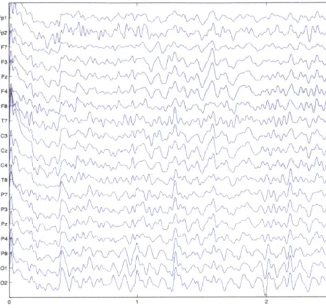
The scalp electroencephalogram (EEG) is a non-invasive tool for measuring electro-physiological brain activity near the scalp. Scalp EEG measures electrical potential changes at different locations along the scalp that result from current flow from neu-rons in the brain. Scalp EEG is measured by placing electrodes in a set configuration on an individual's scalp. A single channel of scalp EEG is the voltage or potential difference measured between a single electrode and either a common reference elec-trode (reference montage) or an adjacent elecelec-trode (bipolar montage). These voltages are then recorded continuously at a set sampling rate. Thus, the scalp EEG signal is commonly represented as a multidimensional signal X, where xit is the voltage in

FpI F7 F4 1 7 P3 04 PEI 01 02

V

~...

Figure 2-1: Example of continuous resting scalp EEG

channel

i

at time t. An example of scalp EEG is shown in Figure 2-1.

Because of the physical limitations of the device, scalp EEG doesn't have the

ability to pinpoint the activity of any neuron within the brain. Each electrode is

picking up the activity of tens of thousands of neurons in similar spatial location

and orientation [21]. Furthermore, the strength of the electric potential generated

diminishes with distance, so neurons near the scalp have the most influence. Lastly,

the cerebrospinal fluid and skull surrounding the brain have an attenuating affect on

the potentials generated. As a result, scalp EEG is the measurement of the sum of

field potentials from a population of neurons found mostly near the scalp.

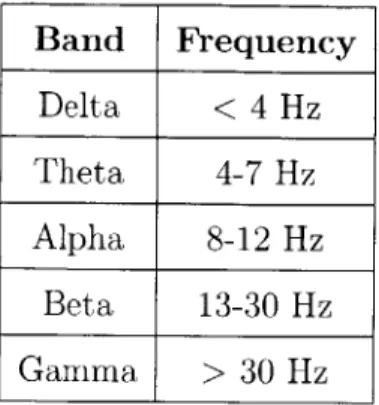
Scalp EEG is commonly described in terms of its frequently identified

rhyth-mic components. The most commonly studied rhythrhyth-mic components of scalp EEG

are identified in Table 2.1. Each of these activity bands have been associated with

different states of brain activity. For example, in awake adults, the scalp EEG is

dom-I K /~r0 N K N P y Cv' ,ii~N' N K N' K"' C 'p iN', ''''C' NI ""C' ~ '~ "N N" CC'' C', N~' \~ V

Table 2.1: Rhythmic Activity Frequency Bands of EEG

inated by Alpha and Beta frequency activity [21]. However, resting scalp EEG is a non-stationary signal in that the power of these frequency bands can vary significantly over the length of a recording.

Scalp EEG is also prone to artifactual noise. These artifacts can be physiological in nature, such as noise from muscle contractions or eye blinks. They can also be mechanical in nature from noise such as power line interference. One must address these artifacts along with scalp EEG's multidimensionality and non-stationarity when doing any analysis with resting scalp EEG.

2.2

Dataset Overview

For these experiments, we used data taken for use in the Collaborative Study of the Genetics of Alcoholism (COGA) [8]. COGA is a ongoing multi-site study with the overall goal of characterizing the familial transmission of alcoholism and related phenotypes and identifying susceptibility genes using genetic linkage. Each subject underwent a psychiatric interview in order to test for a alcohol dependent diagnosis

by three independent criteria. In addition to the clinical assessment and genetic data

collected, a number of of subjects had resting scalp EEG recorded.

The collection procedure for obtaining the EEG is described in [25]. Each signal was recorded for roughly 4 minutes at 256 Hz using a 19-channel montage. Signals were bandpass filtered from 3-32 Hz and eye blinks removed by a frequency-based

Band

Frequency

Diagnosis

Males

Females

Negative for Alcohol Dependence

36

200

Positive for Alcohol Dependence by DSM-III-R and Feighner

492

255

Negative for Alcohol Dependence with some symptoms

154

295

Table 2.2: Summary of COGA subjects with resting EEG listed by alcohol dependence

diagnosis

procedure by [13, 14]. Also, 1 second sections of EEG that had an abnormally high

amount of artifacts were removed.

A summary of the makeup of the subjects for which we have resting EEG data

is in Table 2.2. For consistency with earlier studies [25, 24] using these data, we

chose to use the "COGA Criterion" for alcohol dependence as meeting both the

DSM-III-R [18] and Feighner Criteria [10] for alcohol dependence. These criteria are

listed in Appendix A. An individual is considered to be alcohol dependent by

DSM-III-R if they meet at least

7

of the symptoms listed in Table A.1. Furthermore, a

definite diagnosis for alcoholism is made by the Feighner Criteria if an individual has

symptoms in at least three of the four diagnostic groups listed in Table A.2. Any

subject who was diagnosed as alcohol dependent by both these criteria was considered

positive for alcohol dependence. Our positive population consists of 747 total subjects

(492 males and 255 females).

We chose to only include the 236 subjects (36 males and 200 females) that showed

no symptoms for alcohol dependence in our negative population as we hypothesized

that they would be the most separable from the positive population. There are also

449 subjects that were labeled negative for alcohol dependence by all criteria tested,

but showed some symptoms identified by the criteria in use. Ideally we'd like to

include these subjects as part of our negative population, since this would allow our

positive and negative populations to be much more balanced for model construction

and training. Additionally, we would want our trained models to be able to handle

signals taken from individuals who are "borderline" alcohol-dependent. However, we

I I I I 0.12 0.1 - 0.08-0 2 0.06 0.04-

0.02-Negative for alcohol Positive for alcohol d

29 32 35 38

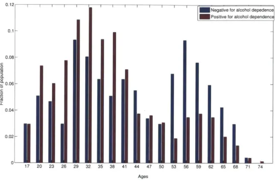
Figure 2-2: Distribution of ages split

III-R and Feighner Criteria

41 44 47 50 53 56 59 62 65 68 71 Ages

I I I I I I

by diagnosis for alcohol dependence by

DSM-found in practice that including these subjects in our negative population decreases

feature correlation with alcohol dependence and lowers performance of trained models.

Thus, for the purposes of this thesis, we did not include those subjects in our further

analysis.

We identified age and gender as two major covariates that would affect the features

we extracted from the resting EEG, and therefore the training of generalizable models.

Age has a significant effect on the periodic features of resting EEG, and this effect

is different in males and females [6]. Furthermore, there are substantial differences

in the distribution of ages between the negative and positive subject populations

(p-value

<

.00001), highlighted in Figure 2-2. We discuss how we control for both

age and gender to train models that will perform better for a general population in

Chapter 5.

At the time of writing this thesis, we only have data for subjects that come from

"Stage II" COGA families, meaning that they contain at least 3 or more primary

relatives who are alcohol dependent. There is additional data from control families

17 20 23 26

depedence

ependenc

that were recruited independently to represent the general population, however, we

do not have access to that data at this time. Having the control family data would

provide the benefit of having "cleaner" controls that don't have a high degree of

family history of alcohol dependence, as well as having more data in areas where our

current dataset is lacking, specifically in our population of males who are negative for

alcohol dependence.

In this chapter, we gave an overview of the types of data that we are using for our

experiments as well as some information about the population of subjects from which

these data were recorded. We also identified two major covariates that we must deal

with when using these data. In Chapter 3, we discuss how to take a resting EEG

signal for a subject, and convert it to a fixed-length feature vector that will then be

used as input to the machine learning algorithms used to train our discriminative

models.

Chapter 3

Feature Construction

Because of the high dimensionality and noisy nature of EEG signal, we cannot simply train machine learning models on the raw data signal. Instead, we extract features that we hypothesize to be useful for training models specific to our task. This gives us the advantage of reducing our long, variable length signals to manageable fixed-sized feature vectors. Furthermore, we try to prune away a large part of fluctuations in the signal that we hypothesize are not helpful for this task. In this chapter, we present a description of the feature extraction process that we use to convert each resting EEG recording into a fixed length feature vector.

3.1

Overview

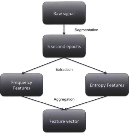
We present a general overview of the process for converting each EEG recording to a fixed length feature vector in Figure 3-1. First, we segment each signal into small "quasi-stationary" epochs. Secondly, we extract multiple types of features from each epoch individually. Finally, we aggregate the features across all epochs to get a single feature vector.

I

Extraction

Aggregation

Figure 3-1: Overview of the feature extraction and aggregation process

3.2

Segmentation

Spectral information within a resting EEG signal can change quite rapidly over the

course of a recording, however, it is commonly assumed that within small

"quasi-stationary" windows, the spectral information from EEG can be meaningfully

mea-sured [3]. Therefore, continuous resting EEG signals are commonly segmented into

smaller epochs before feature extraction [2, 1]. We chose to segment the recordings

into non-overlapping five second epochs. We hypothesized that this would be short

enough to get the desired "quasi-stationary" property, yet long enough to get useful

information about periodic components within each epoch. Lengthening or

shorten-ing the epoch size by a few seconds had minor effects in the resultshorten-ing feature values.

This methodology segmented each recording into approximately 50 epochs.

We also experimented with using an adaptive segmentation procedure described

values after aggregation, and therefore we did not further this method.

3.3

Feature Extraction

After segmenting the signals into discrete epochs, we extract features from each seg-ment individually. Features are extracted from each data channel independently. This allows for channel dependencies to be learned in the training phase described in Chapter 4. Since we use linear classifiers in our training phase we can then directly use feature weights of trained models to see which channels are most useful for our task. A problem with this approach is that we cannot exploit non-linear dependencies between features that cannot be approximated linearly. However, because of restric-tions on how much training data we have available, we felt that it was best to use linear models since they are least prone to over fitting.

As discussed in Chapter 1, there isn't previous work on using machine learning to identify alcohol dependence from resting EEG, and therefore there isn't previous work to build upon for identifying which features within the EEG would be useful to a machine learning classifier. Therefore, we chose to explore a variety of features that have either been shown to be correlated with alcoholics in resting EEG by previous studies or have had use in other discriminative tasks using resting EEG.

3.3.1

Filter Band Energy

The first set of features we focused on were derived from the energy of the signal in different frequency bands. Band power is commonly examined when looking at resting EEG [23]. It gives the strength of the signal at identified periodic compo-nents. Rangaswamy et al. [25] focused on three frequency bands in the Beta range of the resting EEG, and was able to find a significant correlation of band power and alcoholism in resting EEG recorded from males. We chose these three bands (Beta

1 12.5-16 Hz, Beta 2 16.5-20 Hz, Beta 3 20.5-28 Hz) as a starting point for features

to examine and get a baseline performance measurement. We additionally explored including features from the Theta (3-7 Hz) and Alpha (8-13 Hz) bands, since they

have also been shown to be correlated with alcohol dependence [24, 23], although

these correlations haven't been shown to be as strong as those from the Beta bands.

The extraction procedure for the filter band based features is as follows:

1. Normalize signal to have zero mean

2. Filter the signal at the filter band of interest (e.g. Beta 1 12.5-16 Hz)

3. Calculate total energy in that band as the sum of the absolute value of amplitude

of the signal:

n

_J

_{u(n) I}

where u(n) is the resting EEG amplitude at point n.

3.3.2

Approximate Entropy

We also considered features within the signal that are not frequency based. This

allows us to explore information in the resting EEG that is not captured in the

filter band features, and improves model performance when used in conjunction with

the frequency-based features. We focused on the approximate entropy of the signal,

which is an estimate of the unpredictability of time-series data in the presence of

noise [15]. Additionally, we extract the entropy features from the raw signal instead

of the signal at different frequency bands to avoid information overlap with the filter

band energy features. Approximate entropy has been shown to be useful in training

other discriminative models using resting EEG [26], and is calculated by the following

procedure on a time series u(i) with N data points:

1. Choose m, the length of comparison, and a filtering level r.

2. Form a sequence of vectors

x(1),

(N-m+

x(i)

[u(i),

), . . . , U( +

- 1)].

3. Calculate C7'(r) for every i where 1 < i < N, which is defined as the number of

4. Define #'(r) =

(N

5. Calculate approximate entropy as O"'(r) -

#Om+l(r)

On our data, choosing m = 2 and r = 5 gave good variation in measured entropy both within a signal across epochs, and across signals from different subjects. We hypothesized that this variation would make it easiest for models to separate subjects based on these features.

Intuitively, approximate entropy is measuring the log likelihood that patterns within the signal will be followed by similar patterns [19]. An extremely repetitive signal should have an approximate entropy value of near zero, while a more "chaotic" signal should be much higher. We chose to include these features since they represent information to be gained from the inherent randomness contained within the EEG signal compared to the filter band features which measure an estimate of spectral information.

3.4

Aggregation

After extracting features from each epoch, we aggregate information across all epochs in order to produce a single feature vector observation per EEG recording. We could stack all features from each epoch into one long feature vector, however, this formu-lation is not ideal for this application for a few different reasons:

" Some recordings had epochs removed due to abnormally large amount of arti-facts, and as a result not all EEG recordings have the same number of epochs. Thus, each resulting stacked feature vector would not be the same length. " Stacking feature vectors would put an implicit ordering on epochs within a

signal, and therefore would essentially put a relative time enforcement on com-parison between two different recordings. It is unlikely that the relative time of one recording has any meaning within another, therefore this ordering would likely be detrimental to training models that generalize.

* It would make the feature space quite large, increasing the probability of

over-training during model construction phases.

Instead we aggregate information across all epochs without implying a specific

ordering as well as summarizing this information in order to not increase the size

of the feature space dimensionality by a large margin. We explored a few different

methods for aggregating the value of a feature

f(i)

across n epochs. For simplicity,

we held the aggregation method constant across feature type.

Average: The mean value of a feature across all epochs, 1

f(n).

Ragnaswamay

et al.

[25]

aggregated band powers across epochs by simple averaging, and found

significant correlations of these average values with alcoholism. However, mean

values can easily be skewed by extreme values, and provide little descriptive

information about the underlying distribution of values.

Percentiles: The value that is greater than p percent of epoch values for that feature.

By taking values for a feature at various percentiles, we can find information

within the distribution of values across epochs lying elsewhere besides the mean.

For example, it could be the extreme feature values found throughout the length

of the recording that contain the most information. The more percentiles you

use, the closer you come to approximating the cumulative density of the

un-derlying distribution of values, at the cost of increasing the size of your feature

dimensionality.

We also experimented with fitting a distribution to each feature across epochs,

and then using that distribution as the new set of features. However, we found that

in practice this offered little to no increase in correlation with alcohol dependence.

Using a fitted distribution also increases the size of the feature space substantially. For

example, if using a simple histogram with 5 bins to fit a distribution to each feature,

we automatically multiply our feature space by 5. We found that the little amount

of information gained in combination with the increase in feature dimensionality led

to worse performance in practice, and thus we did not further explore using fitted

distributions to aggregate features across epochs.

In this chapter, we discussed how we take each continuous multichannel signal, and convert it to a fixed length feature vector. We first segment each signal into quasi-periodic epochs. We then extract features from each channel in each epoch, and aggregate these features across all epochs. We extract multiple types of features in order to capture different information about variations in the underlying signal, and try multiple ways of aggregating these features across epochs. In the next chapter, we introduce the experimental design used to train our supervised machine learning models on the feature vectors, and test their performance in order to estimate how well they will generalize.

Chapter 4

Experiments and Results

After extracting features from each signal we use these features to train discriminative models. These models can then be used to identify whether if unseen data has come from an alcohol dependent individual. In this chapter, we present our methodology for training supervised models on the features we extracted from the resting scalp

EEG signals, and for estimating how well these models will perform on new data. We

also highlight how these models perform on different populations within our dataset, and which features are most useful for separating alcohol dependent subjects from others.

4.1

Experimental Design

4.1.1

Overview

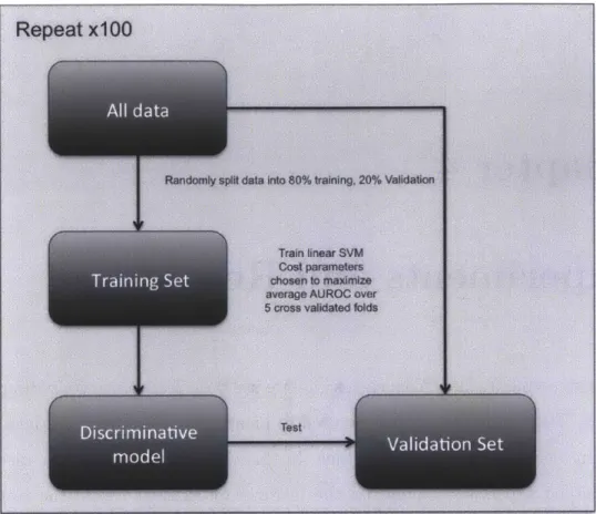
A basic overview of the experiments carried out for model training and evaluation

is presented in Figure 4-1. For each experiment, we take the data from all feature vectors resulting from feature extraction and aggregation. We randomly choose 80% of the feature vectors to be part the "training" set and leave the other 20% out for a "validation set." This is done in a stratified manner to preserve the original ratio between positive and negative examples. We then train a linear Support Vector

Figure 4-1: Overview of the model training and evaluation process

that model's performance on the held-out validation set. Each experiment is repeated

with 100 different random training/validation splits in order to calculate variation of

model performance, and to reduce the effect of particularly "easy" or "difficult" splits

on performance measures.

4.1.2

Preprocessing

Before training, we attempt to control for the effects of age and gender on the resting

scalp EEG features. As discussed in Chapter 2, both age and gender have significant

effects on the periodic features of resting scalp EEG. We do not want our models to

train on these effects because we do not want our model performance measures to be

influenced by information outside of that contained within the EEG signals.

Gender

We handle gender in the same way as previous COGA studies [25, 24] by simply separating the male and female populations. This means that a separate discrimi-native model is trained for each gender. While this trivially controls for any gender related differences in the EEG features, it has one major disadvantage: separating the models reduces the amount of data used to train a classifier, leaving each gender-specific classifier more prone to overfitting. This problem is most serious in the male population, where we have 492 alcohol dependent subjects, but only 36 subjects who show no symptoms of alcoholism. Thus, the model trained on males will suffer from a lack of data in the negative class. However, we found that the differences in resting

EEG between genders were great enough that training a model on the combined set

of males and females led to poor model performance.

Age

There is a fairly wide range of ages (18-73) for the subjects, and thus building popula-tion specific models as we did to control for gender related differences is not feasible. Additionally, we cannot simply include age as a feature since we want our models to train on information from the resting scalp EEG alone. Instead we try to control for the age-related differences in resting EEG features by two different methods:

Matching: With this method we downsample the population of subjects so that the

positive and negative populations are age-matched within a chosen tolerance before model training. This is similar to the previous age-matched studies with the COGA EEG data [25, 24]. This ensures that the model will not train to any age-related differences within the EEG. However, this significantly reduces the number of observations used in the training set, and thus makes trained models more prone to overfitting to noise within the data. Reduction in the number of examples affects the models trained on the male population the most. For the males, using a 80% training, 20% validation split of the data, the age-matched training set will have fewer than 60 examples in it.

Detrending: We use linear detrending to try to decouple the age-related changes

within the features before model training. This methodology was shown to

be successful at removing age related differences in medical imaging data

[7].

We use a class-balanced set of training examples to train simple linear

regres-sions for predicting features from ages. We then use the coefficients from those

regressions to subtract out the effect of age on each feature from the entire

pop-ulation. However, if an accurate regression model cannot be used for finding

the relationship between age and EEG features, this method will not be able to

successfully correct for age.

Both methods have advantages and disadvantages, so we perform separate

exper-iments with each of them to find out which works the best in practice.

4.1.3

Training

In the training phase of the experiment, we train SVMs using a Li-regularized, L2-loss

formulation, which solves the following primal problem:

min

wi

1

i=1

where yi is the label for observation xi, and

denotes the 1-norm. Using

Li-regularization can be useful in applications where the number of features is high and

the number of examples is low enough that overfitting is a potential issue [20]. The

Li-norm returns a more sparse solution than a traditional L2-regularized SVM, and

as a result can help remove the influence of inconsequential features during training.

We chose this formulation because a large number of features, such as features coming

from adjacent channels, are correlated with each other and thus provide redundant

information. The sparse solution returned by the Li-regularized SVM helps mitigate

this problem by eliminating the influence of some features and therefore reducing

overfitting to noise within the training set. If we had more training examples to

mit-igate overfitting, or less redundancy in our features, then a traditional L2-regularized

We use a class specific cost parameter C to account for the class imbalance within our populations. We employ a two-dimensional grid search to find the class spe-cific cost of misclassifications for LIBLINEAR since we don't have a priori knowl-edge of the optimal tradeoff between misclassifying positive and negative examples. We do this using a 5-fold cross validation for each combination of cej, c-j where

+ and - indicate class and i and

j

c E {io-4, 10-3,

10-2, 10-', 1/2,1,2, 10}.

ap-proximately equal size folds. Then we train 5 separate models where 4 of the 5 folds are used to train the model, and the remaining fold is used to test the model's per-formance. We average model performance across the 5 separate models in order to get an estimate of model performance for a given set of hyperparameters. We repeat the cross validation 20 times in order to get a more stable measure of performance for each set of cost parameters within the grid search, and measure the average AUROC on the test set for the 20 repeats of 5-fold cross validation. The set of parameters with the highest average AUROC is chosen and used to train a model on the entire training set.

4.1.4

Feature Selection

As discussed in Section 4.1.3, a large number of features are correlated with each other. This redundancy makes our models prone to overfitting when training. Part of the susceptibility to overfitting is mitigated by the LI-regularization, but it's possible that directly eliminating features could further aid in mitigating overfitting and increase model performance on the validation set.

We experimented with using a basic weight based thresholding feature selection. We first examine the feature weights of a model. We then remove any features with an absolute value less than a threshold, and retrain the model. We set this threshold to be t*Wmax, where Wmax is the maximum absolute value feature weight after the initial

training, and t is a tuning parameter between 0 and 1. We implemented this procedure with the hope of eliminating some features that only contained a non-zero weight due to noise within the training set. This will ideally increase the generalizability of the

trained model, and increase performance on the held out validation set. We found

that choosing a threshold parameter value t of .25 gave desirable results in practice.

We also experimented with a greedy weight-based feature selection approach to

prune away unimportant or highly correlated features. After choosing the model with

the best average cross validated AUROC, we remove the feature with the lowest

abso-lute weight. This procedure is iteratively repeated until only one feature is remaining.

We then choose the set of features that has the best average cross validated AUROC.

This approach produced similar results to using thresholding based feature selection,

and it required much more time to run. Therefore, we decided to solely focus on the

thresholding based technique in subsequent experiments.

We train a model on the entire training set using the found cost parameters and

features. Training sets in the cross validation and final training phase are adjusted for

age by either matching or linear detrending immediately before running the LIBSVM

training procedure to account for age influence within the features.

4.1.5

Testing

The resulting model was evaluated on the held out validation set. Accuracy, AUROC,

sensitivity and specificity were recorded for each random training/validation split and

then averaged over the 100 randomly stratified splits.

4.2

Results

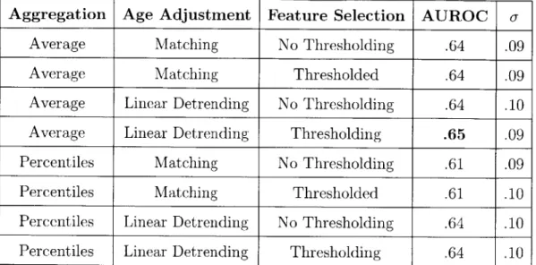
Tables 4.1 and 4.2 summarize the results of the SVM experiments for the different

population of subjects. Each of the performance measures were averaged across the

100 random training/validations splits chosen for each population. These splits were

kept constant across different experiments on the same population in order to ease

comparison of different experiments.

Aggregation

Age Adjustment Feature Selection

AUROC

o-Average Matching No Thresholding .64 .09

Average Matching Thresholded .64 .09

Average Linear Detrending No Thresholding .64 .10

Average Linear Detrending Thresholding .65 .09

Percentiles Matching No Thresholding .61 .09

Percentiles Matching Thresholded .61 .10

Percentiles Linear Detrending No Thresholding .64 .10

Percentiles Linear Detrending Thresholding .64 .10

Table 4.1: Summary of SVM results in Males

4.2.1

Performance of Trained Models in Males

As shown in Table 4.1, we achieve a maximum average AUROC of .65 on the validation set in males. We get the best performance in males when averaging the features across epochs instead of taking percentile values. The percentiles add more information about the distribution of the features across epochs, but they drastically increase the overall size of the feature vector. Furthermore, the weight based thresholding feature selection removes approximately 90% of the features on average, yet has a negligible effect on model performance. This supports our hypothesis that the large number of redundant features makes our models prone to overfitting, and that reducing our feature dimensionality helps increase performance on the validation set.

The average accuracy using the cutoff chosen by the SVM algorithm is 44%. At first glance, this may seem low, considering a random classifier could achieve an accuracy of 50%. However, the class imbalance is so large in the male population, a classifier that always labeled examples as alcoholic would have an accuracy of 93% on the validation set. Therefore, sensitivity and specificity are much more meaningful performance measures for the male population. On average, we achieve a sensitivity of 42% on the validation set, while maintaining a specificity of 81%. Thus, it seems that our model would be able to identify a substantial number of positive subjects

to be alcohol dependent, while still identifying most of the negative subjects as not

alcohol dependent. The sensitivity and specificity of our model are comparable to the

estimated performance of CAGE [11] (sensitivity 43%-94%, specificity 70%-97%).

There is a high degree of variation for the AUROCs across the 100 random folds

for each experiment (standard deviation of .09 for age matched males). Furthermore,

the range between the 5th (.51) and 95 (.81) percentile of AUROC values is quite

high. This wide range of values raises potential concerns about whether the model

would do better than random on unseen data. We believe this is likely due to the low

number of male non-alcoholics used in each experiment (roughly seven in each hold

out set), and that our models should perform better than random on unseen data. To

address this matter, we ran a set of matched experiments where a random classifier

labeled each held out validation set. The results from the models trained with age

matching and linear detrending are both significantly higher than random using the

signed-rank test (p-value

<

.0001). Thus, we believe that we can confidently say that

our model is better than random at classifying subjects as alcohol dependent or not

by their resting EEG alone. Furthermore, we hypothesize that with more examples,

the variation in AUROC across separate training/validation splits would decrease.

4.2.2

Performance of Trained Models in Females

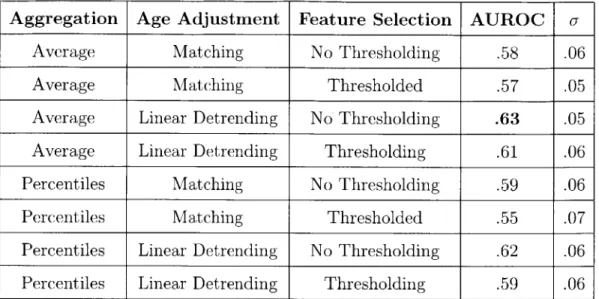
Table 4.2 summarizes our validation set results in females. Similar to the results we

saw in males, we get the best performance when using the average feature value to

aggregate features over epochs, and when we use linear detrending to remove age

effects before training, leading to an overall average AUROC of .63. Just as in males,

our models significantly outperform (p-value

<

.0001) a random classifier.

Even though the average AUROC we get in females is close to what we got in

males, the two results have some major key differences. The average accuracy we

get using the SVM cutoff in the female population is 59%. This is higher than what

we achieved for the males. This is probably because the female population has a

relatively balanced set of positive and negative examples, as opposed to the males.

While the SVM models on average are more sensitive than in the male population with

Aggregation

Age Adjustment Feature Selection

AUROC

a

Average Matching No Thresholding .58 .06

Average Matching Thresholded .57 .05

Average Linear Detrending No Thresholding .63 .05

Average Linear Detrending Thresholding .61 .06

Percentiles Matching No Thresholding .59 .06

Percentiles Matching Thresholded .55 .07

Percentiles Linear Detrending No Thresholding .62 .06

Percentiles Linear Detrending Thresholding .59 .06

Table 4.2: Summary of SVM results in Females

an average recall of 61%, they are also substantially less specific, with a true negative rate of 57%. If we modify our decision threshold to achieve a similar specificity as in males, the sensitivity in females drops to 36%. Overall, these results suggest that our models perform better on the male population than they do on females.

Another major difference between the results in males and females is the lack of consistency in results across experiments in females. In males, changing the aggre-gation or age adjustment method seemed to have little effect on the validation set results. However, this is not the case in females. The largest difference is when using matching in place of linear detrending for age adjustment. Switching from matching to linear detrending in females leads to a significant (p-value < .0001) increase in

average AUROC. This discrepancy could be due to age being a much stronger covari-ate with alcohol dependence in females than in males. The average age for female alcoholics in this dataset is 34, while the average age for non-alcoholics is 45. Using age as a predictor for alcohol dependence you can get an AUROC of .72 in females. While linear detrending aims to remove any age affects, it is highly unlikely that there is a perfect linear relationship between age and each of the features. Therefore, we may not be removing all of the age information within the features. Because age is so predictive of alcoholism in our population of females, this adjustment may lead to an

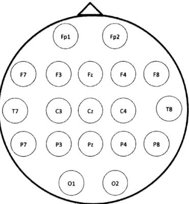
P7 P z 4

01 02

Figure 4-2: Relative location of electrodes along the scalp

artificially high AUROC. However, using age matching is potentially problematic in

females as well. The large differences in ages between non-alcoholics and alcoholics in

females means that a large number of examples are thrown away when using

match-ing to control for age effects. Discardmatch-ing these examples could be the cause of the

decrease in average AUROC. It isn't clear if the results using age matching or linear

detrending best estimate generalization performance, and it's possible that a more

accurate estimate is somewhere between the two results.

Although the results didn't vary as much as in males, we don't get as high of

an average AUROC on the validation

compared to males suggests that the population of females is not as separable as the

population of males within the feature space that we explored. This is consistent with

the findings in Rangaswamy et al.

[25]

where beta power was found to be significantly

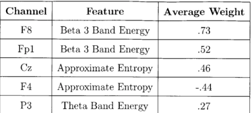
Table 4.3: Top 5 Features in Males by Average Feature Weight

4.2.3

Important Features

Because we use linear models for classification in our experiments, we can look directly at the feature weights to see which features influence the decision value for an example in each model. The features that are consistently given larger absolute valued weights when training models are the most important for identifying alcohol dependence in these data. Therefore, we can see if any particular feature type or channel location (shown in Figure 4-2), is most useful for our task in a given population.

For both males and females, we examine the feature weights of the models trained on features that were averaged across epochs, and that used linear detrending for age correction. We compute the average absolute weight for each feature across all 100 random training/test splits. Weights are normalized to the maximum weight within that model.

The top 5 features for identifying alcohol dependence in males are shown in Table 4.3. Beta 3 energy in channel F8 is by far the most important feature by average weight. This finding is consistent with [25], which identified a significant increase in Beta 3 power in the frontal region in male alcoholics. This is further supported by the second ranking feature in males, which fits into the same category of Beta 3 energy in the frontal region.

Two approximate entropy features in the Cz and F4 channels are also given high weighting on average. This suggests that the addition of the entropy based features to the frequency based features aids in useful information for building classifiers for

Channel

Feature

Average Weight

F8 Beta 3 Band Energy .73

Fpi Beta 3 Band Energy .52

Cz Approximate Entropy .46

F4 Approximate Entropy -. 44

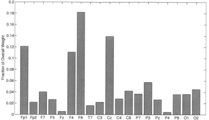
0.2 0.18- 0.16- 0.14- 0.12-6 0.1 0.08 LL 0.06- 0.04-0.02 0 . Fp1 Fp2 F7 F3 Fz F4 F8 T7 C3 Cz C4 C8 P7 P3 Pz P4 P8 01 02 Channel 0.4 0.35- 0.3- 0.25- 0.2-0.15 0

Theta Alpha Beta 1 Beta 2 Beta 3 Approx. Entropy Feature Type

Figure 4-3: Distribution of weights by channel and feature type in males

alcohol dependence on resting scalp EEG in males. Finally, the fifth most important

feature in males is in the Theta band, suggesting that F8 and Fpl provide most of the

information about alcohol dependence that is contained within the Beta frequency

band.

We show the distribution of the weights by channel and by feature type in Figure

4-3. These figures further show that the top features are weighted much higher than

the rest in the models trained on males. After the top 4 channels, the rest of the

channels have close to uniform weight. Additionally, Beta 3 energy and Approximate

Table 4.4: Top 5 Features in Females by Average Feature Weight

Entropy are given significantly higher weight than the other feature types.

Table 4.4 highlights the top 5 important features for identifying alcohol depen-dence in females. In females, features in the alpha and theta bands seem to be the most useful. Beta energy does not seem to be as important in females as in males. This is consistent with [25] that found that the differences in beta power in alcoholics vs. non-alcoholics is not as pronounced in females as it is in males.

Figure 4-4 shows the distribution of feature weights across channels and feature type. The feature weights vary more across the different models trained on the female populations than in the males. Furthermore, the distribution of weights in females is much closer to uniform than in males, especially across feature type. This is supportive of our hypothesis that the female subjects are not as separable as the males within the feature space we explored, since the top features don't stand out from the others as much as they do in males. Additionally, this may help explain why the thresholding feature elimination approach did not increase validation set performance in females as it did in males. If which features are the most important depend highly on the specific observations used to train the model, than feature elimination could hurt overall performance on the validation set.

Channel

Feature

Average Weight

F4 Alpha Band Energy .69

P3 Theta Band Energy -.63

P7 Theta Band Energy .56

F3 Beta

1

0.08- 0.07-0.06 -0.05 0 00.04- S0.03- 0.02-0.01 Thp Fp2 F7 F3 Fz F4 F8 T7 C3 Cz C4 C8 P7 P3 Pz P4 P8 01 02 Channel 0.2 0.18- 0.16- 0.14- 0.12-C) 0.1 .g 0.08- LL0.06- 0.04- 0.02-0

Theta Alpha Beta 1 Beta 2 Beta 3 Approx. Entropy Feature Type

Figure 4-4: Distribution of weights by channel and feature type in females

4.3

Summary

In this chapter, we described the details of how we construct models for identifying

alcohol dependence using resting scalp EEG, and how we estimate the performance

of those models on new data. We trained multiple models on the same sets of data

in order to find how best to preprocess data before training.

In males, our best model achieves an average validation set AUROC of .65, and

for females we get an average validation set AUROC of .63. In both cases we do

sig-nificantly better than a random classifier. Each population raises different questions about the generalizability of results. In males, the standard deviation of AUROC over the 100 different validation sets is quite high. We speculate that this is because there are few negative examples in each validation set, but it casts some uncertainty on how close the performance on new data would be to what we saw on average in our validation sets. In females, we see a lack of consistency in results across ex-periments. There is a major discrepancy between models that use age matching vs. linear detrending to control for the effects of age. We get the best results with linear detrending, but its possible that these results are skewed since age is a good predictor of alcoholism in our set of female subjects, and we may not have removed all of that predictive power from the features when attempting to adjust for age effects.

Because we used linear classifiers when building our discriminative models, we are able to examine the feature weights directly from those models in order to highlight which features extracted from the resting scalp EEG are most useful in identifying clinical diagnoses of alcohol dependence. In males, Beta 3 band energy seems to contain the most useful information, and is supplemented by approximate entropy features as well. In females, Alpha and Theta band energy seem to be the strongest indicators of alcohol dependence, but these features don't stand out from the rest as clearly as the strongest features for males.

In conclusion, we explored a variety of formulations for building models for iden-tifying alcohol dependence in males and females, and our results suggest that we can build models that can do a better than random job of matching clinical diagnoses of alcoholism. In the next chapter, we summarize the work done for this thesis and future directions for further investigating the efficacy of using resting scalp EEG for alcohol dependence diagnosis.

Chapter 5

Summary and Conclusions

Currently there is no physiological measurement that is a clinical indication of alco-hol dependence. Scalp EEG is a tool that has been used extensively for measuring brain activity for neurological conditions such as epilepsy, but its relation to psychi-atric disorders is less clear. Scalp EEG is a noisy, non-stationary signal, but there are established features within a continuous EEG signal that can be extracted from short, quasi-periodic segments that have been useful in building discriminative mod-els. Previous studies have identified features within resting EEG as being associated with alcoholism, but there has been little work in using machine learning to explore resting scalp EEG's relationship to clinical indications of alcohol dependence.

We focused on using supervised machine learning techniques to explore the utility of resting scalp EEG features for matching clinical diagnoses of alcohol dependence. We looked at eyes-closed resting EEG data for 983 subjects from the Collaborative Studies on the Genetics of Alcoholism (COGA) dataset. We first converted each of the continuously recorded signals into discrete feature vectors. We then experimented with training supervised models on a subset of the feature vectors, and measuring performance on a held out test set.

We first considered which features in the resting EEG would be most useful for training discriminative models for identifying alcohol dependence. We chose to extract signal energy at known periodic filter bands since band power has been previously shown to be associated with alcohol dependence. We also calculated approximate