Distributed measures of solution existence and its optimality in stationary electric power systems : scattering approach

(1)

Distributed Measures of Solution Existence and Its

Optimality in Stationary Electric Power Systems:

Approach

by

Kathryn A. Millis

Scattering

B.S.E.E., Northeastern University (1986)

S.M., Massachusetts Institute of Technology (1991)

Submitted to the Department of Electrical Engineering and Computer Science

in partial fulfillment of the requirements for the degree of

Doctor of Philosophy

at the

MASSACHUSETTS INSTITUTE OF TECHNOLOGY

February 2000

©

Kathryn A. Millis, MM. All rights reserved.

The author hereby grants to MIT permission to reproduce and distribute publicly

paper and electronic copies of this thesis document in whole or in part.

A uthor ...

Department cf Electrical Engineering and Computer Science

January 14, 2000

C ertified by ..

...

Marija D. Ilid

Senior Research Scientist, Laboratory for Electromagnetic and Electronic Systems

Thesis Supervisor

Accepted by ...

MASSACHUSETTS INSTITUTE OF TECHNOLOGY

MAR 0 4 2000

LIBRARIES

Arthur C. Smith

Chairman, Department Committee on Graduate Students

(2)

Stationary Electric Power Systems: Scattering Approach

by

Kathryn A. Millis

Electrical Engineering and Computer Science

Submitted to the Department of Electrical Engineering and Computer Science on January 14, 2000, in partial fulfillment of the requirements for the degree of

Doctor of Philosophy in Electrical Engineering

Abstract

Currently, problems of large scale power systems are defined mainly in the voltage-current domain. This thesis introduces an alternate formulation for power systems based on the scattering matrix network formulation. In particular, the load flow problem is defined in the scattering domain. This formulation yields a geometric representation of the equilibrium solution which allows for the determination of more than one solution to the load flow and bounds on system inputs for which a solution exists.

However, as deregulation takes place there is a need for more decentralized comput-ing/decision making. Thus the basic approach to load flow computation is changing be-cause of the lack of centralized information. A byproduct of this scattering formulation is the ability, through local measurements at one bus, to obtain information (i.e. voltage and current) about another bus, a valuable tool in competitive power systems. The procurement of this information is done in a completely decentralized manner.

Given the move toward competitive electricity markets, transmission capacity measures, which tell whether power transfers can be made on the system, have become increasingly important. In the thesis, the scattering versions of LBTC (Load Bus Transmission Capacity) and GBTC (Generator Bus Transmission Capacity) are defined. Proof of concepts were illustrated on a three bus system.

Thesis Committee:

George Verghese, Committee Chairman

Professor, Electrical Engineering and Computer Science Marija D. Ilid

Senior Research Scientist, Laboratory for Electromagnetic and Electronic Systems Bernard C. Lesieutre

(3)

Dedication

This thesis is dedicated in loving memory of

HELEN A. MILLIS

MARY B. KUSTKA

DR. CYNTHIA D. MILLIS

Although my Mother, Aunt and Sister all died before this thesis was

fin-ished, their encouragement and understanding (especially my sister's)

made this endeavor possible. I owe them a great deal of thanks for their

love and support.

(4)

I would like to thank a number of people for their help in the research and writing of this thesis.

Foremost, a special thanks to my advisor Marija Ilid who had the initial idea which led to this thesis. Her support and guidance throughout this project were invaluable. I also owe my gratitude to Bernie Lesieutre and George Verghese, members of my thesis committee, who enriched my work through constructive feedback.

This thesis would not have been possible without the support from a variety of sources. I am grateful to all the sponsors of my academic, research and thesis work, including funding from the Multi-Sponsored Consortium/New Concepts and Software for Competitive Power

Systems. In particular, I want to recognize the following fellowships: Corning Glass, Arthur L. Townsend and Vinton Hayes.

I thank my many friends at LEES. I am deeply grateful to Vivian Mizuno, the admin-istrative secretary who has always willingly helped me over the years. I would also like to thank Vivian, Karin Janson-Strasswimmer and Kiyomi Boyd, members of the administra-tive staff of LEES, and Sharonleah Brown, a former LEES staff member, for their friendship and guidance. I must also thank my friends at EECS, Monica Bell, Lisa Bella, Claire Benoit, Peggy Carney, Betty Maksutian and Marilyn Pierce for their help and encouragement.

Grateful acknowledgements also go out to Vahe Caliskan, Dave Perreault, James Hocken-berry, Ujjwal Sinha, Karen Walrath, Phil Yoon, Petter Skantze, Pooengsaeng Visudhiphan and Jama Mohamed for all of their help and friendship in the lab. In particular, the Latex and WinEdt help provided by Jama gave me the freedom to work on my thesis from home. I am indebted to Poonsaeng for the research that she did on Microwave Theory for the appendix of this thesis. I owe thanks to Petter for the stimulating discussions we had on the real world applications of scattering parameters.

On a more personal level, I offer my sincere and heartfelt gratitude to my MIT "family" members. The friendship, understanding, and encouragement of Mary Jane Boyd, Bruce Wedlock and Virginia Pochetti helped me survive the many challenges of MIT. Mary Jane helped me to survive many a course at MIT. Bruce was a godsend in procuring my Arthur L. Townsend fellowship and for providing me with TA's. Virginia was my "port in a storm" standing with me through the hard times and always encouraging me with her genuine smile.

Finally, I wish to acknowledge my family. To my Father, Andrew, whose love, care, and understanding have always been crucial to my education, THANK YOU. Your many late night trips chauffeuring me to MIT made completion of this project possible. Also, for the love and support of my Brothers, Andrew and Richard, I am deeply grateful.

(5)

List of Figures

2-1 One-Port and Terminal and Network Constraints Configurations . . . . 2-2 2-3 2-4 2-5 2-6 2-7 2-8 3-1 3-2 3-3 3-4 3-5 3-6 3-7 3-8 3-9 3-10 3-11 3-12 3-13

Load Models for One-Port . . . . One-Port Structure . . . . One-Port Example: Constant Impedance One-Port Example: Constant PQ Load Two-Port Representation . . . . Two-Port Example . . . . Two-Port Example: Constant PQ Load

Load

Network of

1

Generator and 2 Buses . . . . One Generator, 2 Load Buses . . . . Base Case: LOAD FLOW INPUT and OUTPUT FILES Base Case Scattering Results . . . . LOAD FLOW INPUT and OUTPUT FILES . . . . Approach I Scattering Results . . . . Three-Port Example: Bus 2 P and

Q

Circles . . . . Three-Port Example: Bus 2 P and

Q

Circles: Blowup Three-Port Example: Bus 3 P and

Q

Circles . . . . Three-Port Example: Bus 3 P and

Q

Circles: Blowup Approach III Scattering Results . . . . Approach III Scattering Results . . . . Approach III Scattering Results . . . .

30 35 36 42 42 44 46 51 59 72 74 75 77 78 79 79 80 80 81 82 83 . . . . . . . . . . . . . . . . . . . . . . . . . . . .

(6)

Scattering Signal Flow Graph of a Three Bus System . . Scattering Signal Flow Graph of a 4 Bus System . . . . 5 Bus Case: Base Case: LOAD FLOW INPUT FILE . . 5 Bus Case: Base Case: LOAD FLOW OUTPUT FILE 5 Bus Case: LOAD FLOW INPUT FILE . . . . 5 Bus Case: LOAD FLOW OUTPUT FILE . . . .

Example I Decentralized Approach . . . . Example II Decentralized Approach . . . . Example III Decentralized Approach . . . .

5-1 Two-Port: Tangency Point Geometry, P2 Circle Inside P3

Two Bus Example: Tangency Point at Bus 2 (P2 and Q2 circles) Two Bus Example: Tangency Points of P2 and Q2 circles . . . .

Scenario One: P2 Circle Outside P3 Circle . . . .

Scenario Two: P2 Circle Inside P3 Circle . . . .

. . . . 125

. . . . 126

. . . . 130

Three Bus Example: Tangency Point at Bus 2 (P2 and P3 circles) . . . . . Three Bus Example: Tangency Point at Bus 2 (P2 and P3 circles) - Blowup Three Bus Example: Tangency Point at Bus 3 (P3 and P2 circles) . . . . . Three Bus Example: Tangency Point at Bus 3 (P3 and P2 circles) - Blowup Example I: Tangency Points of P2 and P3 circles . . . . A-1 Incremental approximate equivalent circuits for TEM transmission lines . . A-2 A transmission line terminated in a load impedance ZL . . . . . .. . 132 132 133 133 134 142 147 3-15 3-16 3-17 3-18 3-19 3-20 4-1 4-2 4-3 . . . . . 85 . . . . . 88 . . . . . 92 . . . . . 93 94 . . . . . 95 113 114 115 5-2 5-3 5-4 5-5 5-6 5-7 5-8 5-9 5-10

. . . .

(7)

List of Tables

3.1 Base Case Transmission Line Data . . . .. . . . . . 73

(8)

(9)

Chapter 1 Introduction

The operation of today's electric power system requires that generation supplies the time-varying load plus transmission losses, bus voltage magnitudes remain close to their rated values, generators operate within specified real and reactive power limits and transmission lines transfer power within their thermal and stability limits. However, an electric power system is never at its equilibrium. Power system dynamics in normal conditions are driven primarily by changes in demand. Typical demand varies on a daily, weekly, monthly and yearly basis and is approximately as predictable as the weather. To meet the anticipated demand, economic dispatch and unit commitment, compensation for transmission losses and meeting static operating constraints are services provided by all generating units. Small random deviations from anticipated demand are handled by automatic generation control which involves changing the set point of governors on some generators.

The main objectives of real-time operation of the electric power system are to schedule maintenance of power plants, turn them on and off and change generation outputs as re-quired to supply the predicted system demand. Since generators cannot be instantly turned on and produce power, generating units must be scheduled in advance in order to meet sys-tem demand and have an adequate reserve margin should generation or transmission line outages or demand exceed the anticipated amounts. The units are chosen such that the expected total cost over a specified time horizon is optimized. Necessary parameters used in determining the turn on and turn off times for scheduling generation include start up

(14)

costs, rates of response and must-run times. In order to meet these objectives, a system operator uses a variety of static network and generation modeling tools which include load flow studies, economic dispatch simulations and optimal power flow (OPF) analyses. Each of these tools assumes that the demand is known which is only true within the accuracy of the forecasted variables, in particular load and unit outage statistics. Typically the power system operates in a stationary condition with slowly varying loads (on the order of hours) and a minimal random load fluctuation, typically under 1%. Thus most of the time dy-namics play no role and can be disregarded in stationary analyses. This thesis is mainly concerned with an alternate load flow model. In particular, the problem will be reformu-lated in the scattering domain and argued that this domain is a more natural basis in which to define power transfer processes.

In this chapter, the conventional load flow problem will be revisited in the voltage-current domain. Depending on how the load flow equations are interpreted, whether as a set of nonlinear equations, finding the zeros of a function or as a mapping, leads to a variety of approaches and techniques to solve the equations. A number of the techniques and approaches will be reviewed along with their strengths and weaknesses. With this as a background, the motivation behind why a scattering formulation was proposed will be discussed.

1.1 Stationary Analysis- Conventional Load Flow

Load flow (stationary) analysis is primarily concerned with the problem that generation must supply the load and accompanying transmission losses. Since the load is generally specified in terms of real and reactive power and the generators are power sources as op-posed to independent voltage or current sources, the load flow equations are formulated as a set of non-linear algebraic equations. As demand and/or unexpected equipment contin-gencies occur, the basic question is whether the system can sustain its operations under the new set of conditions, i.e. does an equilibrium under the new conditions exist. This question is typically answered by performing a load flow study which answers the question of solution existence of the new equilibrium point. This question of solution existence of

(15)

1.1. Stationary Analysis- Conventional Load Flow

a new equilibrium and its properties as contingencies occur is a major concern in power systems operations. For example, if a particular generator or transmission line goes out, a load flow analysis can be used to determine a priori where the problems will occur and thus can be used to develop strategies to overcome the problems. Load flow analyses are also important in planning.

The complexity of obtaining a solution to the load flow equations arises because of different types of data specified at the buses. In particular, loads can be described either as constant impedances or constant real and reactive power (PQ) loads; generators can be modeled as a voltage source (slack bus) or by its real power and voltage magnitude (PV bus). This mix of variables, admittance, voltage, real and reactive power implies that the load flow equations be written in what will be defined as the conventional voltage, current

(V-I) domain in order to distinguish from other approaches that will be discussed. The load flow equations are nothing more than the power balance equations written at each bus with the exception of the slack bus. Thus the power balance equations at bus i are as follows:

n

Pi = |VI|Vj|[gii cos(6i - 3_{j) + bij sin(6i}_- _j)] _(1.1) j=1

71

Qi = E Vi||Vj|[gi jsin(Si - 6j) - bi cos(6i - 6j)] (1.2) j=1

for all i = 1, ...n where P is the real power at bus i,

Qi

is the reactive power, JViI is the bus voltage magnitude, gij and bij are the line admittance parameters and 6_{i is the bus}

voltage angle. Since the important variables at each bus in an electric power system are voltage, magnitude and angle, real and reactive power, the solution to the load flow yields the voltage magnitude and angle at a PQ bus and the angle and reactive power

Q

at a PV bus.

A typical approach to obtaining a solution to the load flow equations is to apply a nu-merical technique [26]. One of the nunu-merical algorithms used in solving the conventional load flow is the Newton-Raphson method. Since the load flow equations defined in equa-tions (1.1) and (1.2) can be written as F(x) = 0, the Newton-Raphson algorithm involves 15

(16)

a Taylor series expansion of F around an operating point:

xk+1 Xk j(Xk )F(Xk)

where xk and xk+l are the values of x at the kth and (k+1)th steps respectively, J(xk)-1 is the inverse of the Jacobian &F _ax at Xk. Because it is a numerical algorithm, the Newton-Raphson method may fail to converge to a solution if the Jacobian is singular, [27] the initial guess is outside the region of attraction of the solution or there is a limit cycle problem. It is noted that if the algorithm does not converge, there is no way of knowing whether there is no solution or one of the previous conditions exists.

Since the computation time of the Newton-Raphson algorithm is on the order of

n3,

use of this methodology would not be practical for very large power systems [2]. However properties of the electric power system are exploited in order to reduce the computation time. The structure of a typical power system is such that it has fewer than three lines connected to each bus [2]. As such, the bus admittance matrix of the transmission system,

YBUS, has a small number of nonzero elements, i.e. it is sparse. Many load flow programs

employ sparse matrix techniques to reduce the time to solution convergence.

1.2 Stationary Analysis

-

Alternative Approaches

One way to view the load flow equations in ( 1.1) and (1.2) is that they are a set of nonlinear algebraic equations. However, as previously detailed, they can also be interpreted as a set of equations F(x) = 0 where the objective is to find the zeros of the function F(x). A third interpretation is that the function F(x) is a mapping of R' -+ Rn. Each of these

interpretations leads to different approaches in solving the load flow and there is extensive literature detailing these approaches [22, 23, 24, 25]. Simplifying assumptions based on characteristics and properties of the electric power system that lead to simpler models are what will be described as modeling approaches. These include the decoupled and DC load flow problems. Finding the zeros of F(x) is usually accomplished via iterative techniques, i.e. Newton-Raphson, Gauss-Seidel. Viewing F(x) as a mapping leads to continuation

(17)

1.2. Stationary Analysis -Alternative Approaches

algorithms and homotopy methods. There have been a number of approaches taken to simplify and solve these equations either from the perspective of modeling assumptions or from the choice of numerical technique. This section will present a brief summary of some of the common modeling and numerical techniques that are used.

1.2.1 Modeling Approaches

From the electrical characteristics and inherent properties of the electric power system in normal operation, many simplifying assumptions can be made to obtain either simpler models to be used for computing the load flow or a simpler set of load flow equations. In this section a number of approaches, namely the decoupled real power/angle load flow problem, the decoupled reactive power/voltage load flow problem and the nonlinear resistor network interpretation of the real power/angle load flow problem will be reviewed [28]. Exhaustive and extensive descriptions of other approaches including applications of the above approaches in the deregulated industry are found in [1]. However, the main purpose of all of these approaches is to find a solution to the load flow equations. Due to the nonlinearity of the equations and potential difficulties in applying standard numerical techniques such as Newton-Raphson discussed above, attempts have been made to simplify the equations through modeling assumptions about the physical characteristics and inherent properties of the electric power system. In each of these approaches, certain assumptions are made about the state of the electric power system (i.e. transmission system, voltage angles and magnitudes and the modeling of loads) in order to simplify the equations. Simplification of the equations allows the establishment of conditions (i.e. bounds on system input and topology changes) under which solutions are guaranteed to exist. Use of a specific numerical algorithm only detects that a solution is not computable.

Since contingencies are a major concern in power system operations, it is necessary to know what power flow changes will occur due to a particular generator or transmission line outage. This contingency information obtained in real time can be used to anticipate prob-lems caused by such outages and to develop strategies to alleviate the problem. Decoupled load flow algorithms have been developed that improve computational efficiency and reduce 17

(18)

data storage requirements. The decoupled load flow approach is based on the premise that most transmission lines are predominantly inductive (the ratio of reactance to resistance is on the order of 10 to 1) and that under normal operations, the angle differences between buses tend to be less that 10 degrees, and voltages are close to 1 per unit [3]. This leads to two observations:

" Changes in the voltage angle 6 at a bus primarily affect the flow of real power P in the transmission lines while the flow of reactive power

Q

is relatively unchanged (P-6 decoupled load flow problem).

" Changes in the voltage magnitude IVI at a bus primarily affect the flow of reactive power

Q

in the transmission lines while the flow of real power P is relatively unchanged

(Q - V decoupled load flow problem).

Under these assumptions, the load flow equations are defined as two lower order sets of decoupled load flow equations because the voltage angle corrections A6 are calculated using only real power mismatches AP while the voltage magnitude corrections are calculated using only AQ mismatches. These approximations are used to simplify elements in the Jacobian matrix and hence the dimensionality of the computation is reduced. The result is that convergence is faster than that of the Newton-Raphson based computing approach of the coupled load flow problem. However it is important to point out that the use of a decoupled load flow generally results in some loss of accuracy in analytical or numerical conclusions of interest. This is of particular noteworthy if the system is subject to significant changes.

If in addition to the decoupling assumptions all the bus voltages are assumed constant at nominal values of 1 per unit, the result is the DC load flow model. If, in addition, the resistive part of the transmission lines is neglected, this formulation can be interpreted as a linear resistive network whose branch parameters are a function of the susceptance of the bus admittance matrix YBUS and whose currents and voltages are replaced by real power flows and phase angles respectively. This interpretation is important since positive resistive

(19)

1.2. Stationary Analysis - Alternative Approaches

networks with independent voltage and current sources always have a unique solution. This guarantees existence of the solution for phase angles under small changes in input power.

There are also properties of the electric power system that are exploited in the imple-mentation of some of these approaches. One property in particular is the localized response property of the P-S power network which is the localized response of a transmission network to changes in real power input [29, 30]. Many algorithms for fast computation of the effects of changes in real power propagation in a large system are based on this property. The lo-calized response property of a transmission network to changes in real power input is based on the fact that changes in voltage phase angles decrease monotonically as the electrical distance from a triggering event decreases. This property is often used by a system operator in deciding which corrective actions to take in the case of a contingency or contingencies.

To further assist the power system operator in the evaluation of possible contingencies is the use of an approximate method known as the distribution factors method. Great precision is not required since the primary interest is in knowing whether or not an insecure or vulnerable condition exists in the steady state following an outage. The distribution factors method is a linear method based on the DC load flow model and is used for assessing the effect of changes in real power line flows. This method uses sensitivities of power flow in the line of interest with respect to the power injection at bus i.

1.2.2 Numerical Approaches

Whereas the previous section discussed modeling assumptions and simplifications, this sec-tion will present a brief summary of some of the numerical tools used in obtaining solusec-tions to the load flow equations. These include continuation methods, embedding algorithms and homotopy methods [22, 24]. The issues involved in choosing the appropriate numerical method are the nature of the nonlinearity, conditions under which the method will converge to the required solutions, the rate of convergence of the iterative scheme, computational speed and computer storage.

The load flow equations in (1.1) and (1.2) can be rewritten as F(x) = 0 where F is a nonlinear function. The only way to find the zeros of the nonlinear function F is to use an 19

(20)

iterative technique

[23].

An iterative approach involves starting with an initial guess and calculating successive approximations to the solution by applying an appropriate iterative technique. However, iterative approaches may converge slowly (as in the case of Newton-Raphson) and suffer from numerical instabilities and bifurcations.

Rather than viewing the load flow equations as finding the zeros of a nonlinear function,

F(x) can be thought of as a mapping of R" -+ R'. Given this interpretation, an alternative

to the conventional numerical techniques is a continuation algorithm. The basic idea of the continuation method is the idea of gradually deforming a simple (usually linear) problem to a nonlinear one. In the case of the load flow equations, the solution to F(x) = 0 is desired. Since F(x) is a mapping of R' -+ R', the continuation method involves deforming an

arbitrary mapping with a known solution into the mapping F(x) whose solution is x* by varying a parameter. This continuation parameter, defined as A, A E [0, 1], is used to define a new mapping H (i.e. R" -+ R') where

H(x, A) = (1 - A)G(x) + AF(x) = 0

and where G is a trivial map with known solution x'. By gradually varying A from 0 to 1, the continuation method deforms a trivial map G(x) with known solution to the desired problem F(x), whose solution is x*. Thus starting at A = 0, (H(xo, 0) = G(xo) = 0) and increasing A in positive fixed steps results in H(x*, 1) = F(x*) = 0 which is the desired result. Note that the solution space is a curve which is parametric in A, i.e. x = x(A)

and this continuous curve in R' starts at the initial point (XO, 0) and ends at the required solution (x*, 1).

Advantages of the continuation method are that they may increase the domain of con-vergence of a solution and may also be used to bring the initial guess closer to the solution and within the region of convergence. These advantages are due to the global convergence and convergence to multiple solutions properties of the algorithm.

If the interval is partitioned into k equal subintervals, J = !, then this continuation algorithm is known as the embedding algorithm. Thus starting at the known solution points, the solution space defined by H(x, Ai + 6A) = 0 for i = 1, ... k is solved for x using

(21)

1.3. Scattering Approach to Power Systems -Motivation

an iterative method which applies the xi-I solution as a starting approximation to the ith problem. Under the assumption that (Aj+₁- Aj) is sufficiently small, x - should be a good approximation to xi so that convergence occurs. However, this embedding algorithm does not work well in general.

To overcome these inherent difficulties, the homotopy method is used [25]. This method is generally more robust and exhibits numerically stable characteristics. The reason is that the homotopy curves are always smooth, well-behaved paths. In particular bifurcation points and other ill-conditioned cases may be avoided. This involves a number of restrictions on the mapping H(x, A). The first is to ensure that at least one path exists that will connect the initial solution of the mapping (A = 0) to the final solution (A = 1). This involves determining whether H-1 consists of well-behaved paths that do not intersect themselves. The second issue is to ensure that if the solution exists, the path will always reach a solution and will never tend to infinity. There are many other issues applying the homotopy method to obtain the solution of F(x) = _{0 including ways of embedding a homotopy parameter,} in particular the free-running case, the forced case and globally convergent probability-one homotopy methods.

Continuation methods have been successfully applied in obtaining the solution to the load flow equations. A detailed description of the results is given in [1]. However the key points in applying the homotopy method to power systems are that:

" Generation of multiple solutions is dependent on the type of homotopy mapping. " Starting point on the path determines whether single or multiple solutions will be

generated.

" The method only converges to stable operating points.

1.3 Scattering Approach to Power Systems

-

Motivation

In the previous sections, both the modeling approaches and numerical techniques for solving the load flow equations are defined in the voltage, current domain. The reason for this is that loads are modeled as either constant impedances or as constant real and reactive power

(22)

loads, generators are modeled as voltage sources or in terms of their specified constant real power and voltage magnitude and the transmission system is described by its bus admittance matrix. Thus the load flow equations, which are the power balance equations at each bus (excluding the slack bus) are a mix of voltage magnitude and angle, real and reactive power and admittance parameters. It is this mix of variables that results in the complicated nonlinear algebraic equations that constitute the load flow problem since the common basis in which to represent voltage and power is the voltage, current basis.

In this thesis an alternate approach to modeling a power system is considered, namely the scattering approach. In the most general terms, the scattering approach is concerned with the interconnection of lumped elements or "obstacles" within a flow type process in which flows are partially transmitted, reflected or absorbed at a system boundary. In the scattering domain, the basis variables are the incident and reflected variables which are linear combinations of voltage and current appropriately scaled by a normalizing impedance such that the units of these basis variables are (volt-amperes) 2. The scattering parameter,

defined as the ratio of the reflected and the incident variables, can describe the performance of a system under a specified set of terminating conditions. In particular, questions of power transfer from a finite impedance generator to a load are frequently best handled by scattering relations and it is possible to deduce general theorems for these situations which are hidden when impedance or admittance characterizations are used [4].

The application of the scattering formalism is particularly important because of the non-uniform characterization of loads, generation and transmission in the voltage, current domain. Using the basis variables of incident and reflected waves, load, generation and transmission can be uniquely characterized in terms of scattering parameters and/or a scat-tering matrix for a specified normalization. The conventional load flow equations represent the power balance at each bus, namely that power injected into the transmission system at bus i must match the flows through the transmission links connected to bus i. In the scattering formulation of the problem, generation and load represent boundary conditions at each of the ports of the transmission network. At the boundary, instead of matching power flows, the incident and reflected waves of the transmission network and its ports must

(23)

be matched.

Furthermore, use of the scattering approach introduces an important property which is the idea of separability based on a decomposition of the system into the transmission network and its ports, generation and loads. The transmission network can be thought of as a network constraint whereas load and generation can be viewed as terminal constraints. This separability establishes a mechanism by which local measurements at a bus can be used to deduce information about another bus. This leads to a decentralized approach to the load flow. As deregulation takes place and competition increases, less information will be made public and the basic approach to computation of the load flow will change. In the new deregulated environment, there will be a need for more decentralized computing and decision making and alternative approaches such as the scattering approach will become necessary.

1.4 Contribution of Thesis

This thesis is essentially a proof of concept on the application of a new approach in solving some problems in the electric power system. The contributions of this thesis fall into three sections corresponding to three problems in the electric power industry that were investigated.

The first is the casting of the coordinated load flow problem in the scattering domain. The coordinated load flow is the same as the conventional load flow which is used for feasi-bility and reliafeasi-bility studies. Since the scattering literature is devoted to linear applications, this is the first attempt to separate the linear portion of the load flow problem from the nonlinear port constraints. One of the contributions is to define the nonlinear constraints, i.e. PQ loads, in terms of finding the appropriate intersection points of real and reactive power circles. This leads to the main contribution of a geometric display of the solution at each and every bus which allows for the determination of more than one solution. In contrast to the traditional approach to solving load flow, a numerical algorithm yielding only one solution per simulation, this approach yields additional information about how close the system is to not being solvable. The separation of the two solution points is a

(24)

metric for how close that bus and the system comes to being solvable. Thus, in the case where the two solution points are very close at a particular bus, doing a power transfer from some other point on the system would not be possible.

The second contribution is a formulation of a decentralized load flow problem which involves obtaining information in a decentralized manner. The assumptions made in defining the decentralized load flow problem are that there is a step change in one or more than one of the load parameters and the system settles to a new equilibrium and that transmission

and generation (i.e the slack bus) are known by all players on the system.

The contribution in the decentralized load flow approach is the exploitation of the fact that if the loads and generation are defined in terms of scattering parameters which are a and b, the incident and reflected voltages respectively, the transmission system is defined as b =

Sa, where S is the scattering matrix of the transmission system, the problem is transformed into the scattering domain and solved explicitly in the scattering domain. In contrast to the previously defined approach, the nonlinear port characterizations are transformed into an a, b port characterization. This approach exploits the linear input/output description b = Sa. The nonlinearity of the loads is transformed by characterizing the loads in terms of the incident and reflected powers. Since the problem is now linear, a Gauss approach is used to determine the scattering parameter, IF, at the other bus (in a three bus example).

The third contribution is the calculation of the transfer capacity in the power network using the scattering domain approach. While the conventional approach is to do a DC load flow to approximate the solution, the scattering approach exploits the geometry of the problem by obtaining the tangency points of power circles since the premise is that as the real power is varied, the maximum amount of power that can be transferred to a particular bus is the value of the real power such that the two circles (in a three bus example) are at their tangency point.

The contribution in the calculation of the transfer capacity in the power network is that this is a geometric approach to obtain the load bus transmission capacity as opposed to a straight numerical algorithm.

(25)

1.5. Thesis Overview ₂₅

1.5 Thesis Overview

Chapter 1 reviews the literature on solving stationary analysis (load flow) problems includ-ing both the modelinclud-ing approaches and numerical techniques that are currently known. This review serves as a starting point and establishes the motivation behind why the scattering approach was proposed in this thesis.

In Chapter 2, the scattering parameter and the scattering matrix are revisited using both simple one-port and two-port examples. In particular, the different types of normalization, real and complex are reviewed as this becomes an issue in the case of voltage and reactive power relations. However, the methodology on applying scattering parameters/matrices to power problems is extended in this chapter to include loads that are not simple impedance type loads. The approach in handling loads which have a nonlinear port characterization in the voltage-current domain, namely PQ loads, is detailed for both the one-port and the two-port examples. This defines part of the approach taken in solving multi-bus examples. The approach used to describe these nonlinear loads leads to a novel geometric display of the solution and is illustrated in examples for both the one-port and two-port. This serves as the starting point to characterize the multi-bus coordinated load flow problem in Chapter 3.

Chapter 3 lays the structure for defining the coordinated load flow problem for the multi-bus system. A three bus example is used to illustrate the results. Three varieties of the load flow formulation in the scattering domain, terminal/network constraint load flow formulation, scattering voltage and current load flow formulation and geometric load flow formulations were defined and simulated. The setup of the terminal/network constraint load flow formulation and the scattering voltage and current load flow formulation are similar since both are cast as F(X) = 0 type problems. The geometric load flow formulation exploits the geometry of the problem. Rather than using a Newton-Raphson approach as was done in the previously mentioned formulations, the idea is to generate the intersection points at each iteration in the simulation. Multiple three bus examples verify that each of these formulations yields the same solution. A five bus example consisting of a single generator and four PQ loads is shown to illustrate a multi-bus example. Problems in modeling PV

(26)

elements (generators) are discussed.

In Chapter 4, the decentralized load flow problem is defined. This problem involves obtaining information about other buses on the system using local measurements. Dereg-ulation is changing the basic approach to load flow because of the lack of systemwide in-formation. Thus there is a requirement for more decentralized computing/decision making. The assumptions made in defining the decentralized load flow problem are that there is a step change in one or more than one of the load parameters and the system settles to a new equilibrium and that transmission and net generation (i.e the slack bus) are known by all system users. In this thesis only a single generator multiple load system examples are studied. Generalizations for multi-generator systems requires new modeling of PV elements.

The problem is posed and solved in the scattering domain. This approach exploits the linear input/output map b = Sa. The nonlinearity of the loads is transformed by characterizing the loads in terms of the incident and reflected powers. Since the problem is now linear, a Gauss approach is used to determine the scattering parameter

F

at the other bus (in the three bus example). In the case of the three bus example in the thesis, which is used as proof of concept, it is assumed that characteristics of one of the loads are known. Since it is known, it can be characterized by a, b and hence

F.

The solution to the problem is to solve for F at the other load such b = Sa is valid for the entire system. Three examples

are used to illustrate the approach. Since this approach has applications in the competitive electric power industry, several examples are discussed in detail as to the usefulness of this approach.

Chapter 5 deals with the transfer capacity in the power network. It exploits the fact that solutions to the load flow in the scattering domain can be obtained from the intersection points of circles. Using this geometric approach to the problem, the transfer capacity in the power network is determined by obtaining the tangency points of power circles since the premise is that as the real power is varied, the maximum amount of power that can be transferred to a particular bus is the value of the real power such that the two circles (in a three bus example) are at their tangency point. The geometry of the problem and two three bus examples illustrate this approach.

(27)

1.5. Thesis Overview

Chapter 6 summarizes the contributions of this thesis and discusses further areas of research.

(28)

(29)

Chapter 2 Review of Scattering

Parameters

/Matrices

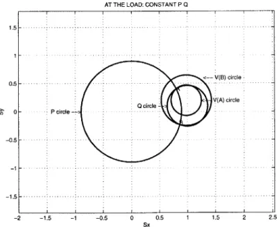
In this chapter, the basic definitions of scattering parameters and matrices will be reviewed for both real and complex normalizations. Given these definitions, expressions for the real and reactive power delivered to a load will be derived. It will be shown that these expressions can be represented geometrically as circles in the scattering plane. Thus, solutions to the network problem will be obtained from the intersection points of the circles. If there are no intersection points, then there is no solution. In particular, examples for two topologies, a one-port and a two-port, will illustrate the application of scattering parameters for obtaining solutions to the network. For the case of the one-port, two different load models, a constant impedance and a constant real and reactive power model, will be explored. In the case of the two-port example, only the real and reactive power model will be illustrated. The cases will serve as a basis to extend the model to three buses which is the content of the next chapter.

2.1 Scattering Approach

Historically, the literature concerning scattering parameters and/or matrices has been di-vided into two areas: applications to microwave problems and applications to specific

(30)

net-REPRESENT BY THEVENIN EQUIVALENT 0

r --- --- --- ---- I

GG1

VI + R

SGENERATOR

ONE PORT DECOMPOSITION: THEVENIN EQUIVALENT

GENCO TRANSCO I

4'

LOAD LSE TERMINAL CONSTRAINT e. VG I GENERATOR TERMINAL CONSTRAINT I / PQ I'A -~ LOAD I I NETWORK CONSTRAINT

TERMINAL CONSTRAINT, NETWORK CONSTRAINTS DECOMPOSITION

Figure 2-1: One-Port and Terminal and Network Constraints Configurations

TRANSMISSION NETWORK _P,Q I TRANSMISSION NETWORK 4*' - - - - -0 I 00 " " " " - ,*#*

(31)

work problems. Scattering theory has its origin in microwave theory. A review of scat-tering parameters in microwave theory is given in Appendix A. Many typical problems are concerned with wave propagation on transmission lines with specified terminations. In microwave circuits, the electric and magnetic fields inside a termination are uniquely deter-mined by either the voltage or the current at the terminals. Rather than representing these fields in terms of their voltage and current, the natural representation is the amplitude of the incident and reflected waves. The amplitude and phase of the transverse component of the electric field in the incident wave are designated by "a" such that

}aa*

represents the average incident power where a* is the complex conjugate of a. The amplitude and phase of the reflected wave are designated by "b". For any incident or reflected wave, the fields are uniquely defined. Given the definitions of a and b, a reflection coefficient, r = , is defined for a particular reference plane or terminal pair. Since there is a connection between the electric field and the magnetic field and the terminal voltage and current, there is likewise a connection between currents and voltages and incident and reflected waves. If "e" is a measure of the total transverse electric field, and "i", is a measure of the magnetic field, it can be shown that e = Ka(1 + F) and i = a(1-r) _K where K is a proportionality factor since a and b are normalized with respect to power. Thus for microwave circuits, scattering parameters are a natural representation for the fields of the incident and reflected waves of a transmission line terminated in a specified structure [5].

Given the characterization of microwave circuits in terms of fields (voltage and current) and scattering parameters, there is a similar analogy between characterizing linear networks in terms of voltages and currents or scattering parameters. The corresponding scattering variables are termed incident and reflected voltages or incident and reflected currents. These are linear relations between the scattering variables and the true voltages and currents in the circuit. Since the scattering parameters of a network describe the performance of a network under any specified terminating conditions, every linear passive, time-invariant network has

a scattering matrix although it may not have an impedance or admittance matrix [10].

The scope of this thesis is the use of scattering parameters in the solution of specified network problems. In particular, scattering parameters have been used to describe the

(32)

formance of a network under specified termination conditions. They have also been used to obtain characterizations of networks since every linear passive, time-invariant network has a scattering matrix. It is noted that the scattering matrix of an ideal transformer exists while its admittance/impedance does not. Particular applications of how scattering parameters and matrices have been used include calculation of the noise figure in negative-resistance amplifiers [6] and classification of lossless three-ports

[7].

Much of the scattering parame-ter/matrix literature is devoted to problems of physical realizability and the synthesis of ideal transformer networks and also applications of scattering parameters to network syn-thesis. There are also a number of specific examples in the literature [9, 10] where scattering parameters/matrices are used in determining the power transfer from a complex generator (defined as a voltage source with source impedance) to an impedance load. The method-ology is to match-terminate at each port, i.e. choosing a normalizing impedance such that there is no incident wave at that port. For example, in the case of a two-port, described by a scattering matrix S, match terminating at ports 1 and 2 means that there are no incident waves at ports 1 and 2. Under these conditions,

1S

21

1

2

,

is interpreted as the forward trans-ducer power gain which is the ratio of actual load power to the maximum power available from the generator when both ports are matched. Since match-termination is defined for the specified load, if the load changes the port has to be match-terminated again. Rather than resolving the entire problem, Youla and Patterno [8], developed a methodology to modify the elements of the scattering matrix. However, these approaches can not be directly ap-plied to power systems since in most cases the loads are not defined as constant impedance but as constant real and reactive power (PQ) loads. These approaches do serve as a starting point to gain intuition in defining electric power problems in terms of scattering parameters and matrices.

In this thesis, scattering parameters/matrices will be applied in a different context, namely using what will be described as a scattering approach to obtain steady state solutions (equilibria) in electric power networks. To understand the ramifications of this undertaking, the results of applying the scattering approach to simple electric circuits need to be studied in order to link the V-I domain to the scattering domain. In this chapter, the scattering

(33)

parameter and matrix is reviewed and applied to both one- and two-port examples.

The scattering parameter approach involves "transforming" the circuit from the V-I domain to the scattering domain via the scattering transformation. Circuit parameters expressed in a V-I context are mapped into a scattering parameter formulation from which real and reactive power and voltage can be extracted. In the one-port example, the approach involves solving the problem at a specified point in the circuit, i.e. at the load or at the generator and assuming a Thevenin equivalent as seen by that point. For the purposes of this discussion, it is assumed that the real and reactive power delivered to the load and the voltage across the load are desired so that the point of reference will be the load.

In this and the next chapter, how the network topology is decomposed, either as a one-port structure or separated by loads and generators from the transmission network, will play an important role not only in the interpretation of the scattering parameter but also in the formulation of the problem. As shown in Figure 2-1, the network consisting of one generator, one load and a transmission network can be modeled either as a Thevenin equivalent driving the load or the generator and load can be viewed as terminal constraints on the transmission network which itself is viewed as the network constraints. It is noted that in the current deregulated vernacular, the generator is defined as a GENCO, the transmission system as a TRANSCO, and the load as a Load Serving Entity (LSE) as shown in Figure 2-1. This decomposition can be extended to multi-ports, however decomposing the network into the terminal and network constraints decomposition lends itself to a more manageable structure.

For the purposes of illustration, the advantages of the one-port structure will be reviewed and two examples using different load models will be shown. With this type of topology, the scattering parameter has a physical interpretation. This can be contrasted to the terminal/network decomposition where the scattering parameter of each port may or may not have a physical interpretation. In particular, the scattering parameter at each port can be interpreted as being a local measure as opposed to the one-port structure where the scattering parameter contains both system and local information. It is this attribute that makes the scattering parameter such a powerful approach in solving these problems. As will be detailed in the sections that follow, system information in the form of the Thevenin

(34)

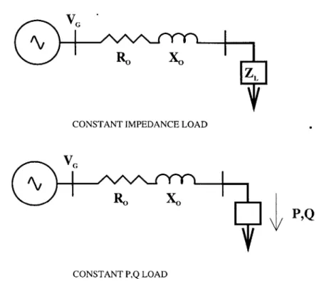
impedance is encoded into the scattering parameter for the one-port formulation. If the problem is defined in a Thevenin structure, the scattering parameter also captures local information, namely the voltage and real and reactive powers at the point of interest. Thus, two independent local variables can be extracted from the scattering parameter via predetermined expressions. To illustrate the advantage of this approach, consider the circuit in Figure 2-2 and assume that the load is described by an impedance ZL. ZL is defined as the ratio of voltage to current so knowledge of one of these variables is necessary to calculate the real and reactive power delivered to ZL. The voltage across the load is obtained via a voltage divider which is a direct result of the Thevenin structure of the problem. However, the voltage or real and reactive powers cannot be obtained strictly from knowledge of ZL and likewise knowledge of the voltage does not imply knowledge of ZL or the real and reactive powers. ZL, voltage, real and reactive powers are all local variables in the V-I domain and contain no system information. By using the scattering approach in the one-port formulation, local information such as the voltage across the load and real and reactive powers delivered to the load is captured in a single parameter for which there is no analog in the V-I domain. Since the scattering parameter formalization depends on the type of load model used, i.e. constant impedance or constant PQ, two different strategies for solving the problem will be derived. For the case of a constant impedance load, a standard approach of applying the definitions of the scattering parameter is used to calculate the real and reactive power delivered to the load and the voltage across the load. For the PQ load, specifying the real and reactive power delivered to the load defines the scattering parameter(s) through which the voltage(s) across the load can be determined. If no scattering parameter can be constructed, there is no solution.

2.2 Review of the Scattering Parameter

The scattering parameter is by definition a ratio of reflected voltage "b" to an incident voltage "a" where the reflected and incident "voltages" are linear combinations of the cur-rents and voltages that have been normalized by a normalizing impedance. Depending on the type of normalization used, real (Z, = R,) or complex (Z, = R, +

jX,),

two different

(35)

VG

(RD

XO

ZL

CONSTANT IMPEDANCE LOAD

VG

Ro

X0

P,Q

CONSTANT P,Q LOAD

Figure 2-2: Load Models for One-Port

"definitions" and uses of the scattering parameter result. For each type of normalization, a set of equations describing the relationship between the scattering parameter and real and reactive power and voltage will be derived. For these derivations it is assumed that the load is a constant impedance and that the resulting expressions can be applied to a PQ load,

the details of which are given in the following section.

In the following two sections, the scattering parameter for a one-port, assuming real and complex normalization, will be derived assuming the network configuration shown in Figure 2-3.

2.2.1 Real Normalization

The network shown in Figure 2-3 consists of a one-port driven by a Thevenin equivalent. The incident and reflected voltages designated as a and b in the figure are defined as:

a = -[ + IL R0]

2 V/RI

(36)

I GEN L a+ V ONE PORT

Figure 2-3: One-Port Structure

b [ VL - IL Ro

2 /R0

where VL and IL are the actual voltage across and current into the load. For the case where the one-port is modeled as a constant impedance ZL, the scattering parameter s is defined to be

b _{ZL - ZO}

a ZL + Zo

It is noted that since Zo is real, the above expression is the same as the reflection coefficient

F

for transmission lines. F is used in determining the voltage and current at any point along a transmission line modeled with distributed parameters. In the literature, the above definition is the most common and in many cares Ro is taken to be one. Given the network configuration in Figure 2-3, the normalization Zo is set equal to

ZGEN-Solving the above equations of a and b for VL and IL yields

VL [a + b]

_[a - b]

(37)

-Since b = sa the above expressions for VL and IL become

VL = a_[1+s]

and IL a [1-s ].

vR0o

The complex power delivered to the load is VLIL* = PL + jQL where * denotes the complex conjugate. Using the above expressions for the voltage and the current, the rela-tionships for the real and reactive power as a function of the scattering parameter are

pL= P₀(1 - SI2) (2.1)

and QL = 2POsy (2.2)

where sy is the imaginary part of s and PO is the power delivered to the load under matched conditions, that is when the load impedance equals the complex conjugate of the Thevenin impedance as seen by the load [11]. The equation relating PL to the scattering parameter is a circle centered at the origin with radius equal to 1 -

(

while the relationship between

QL

and the scattering parameter is a horizontal line in the scattering plane. Since the normalization is the real part of the Thevenin impedance, the voltage across the load is

VL = VGEN

2.2.2 Complex Normalization

Assuming the network configuration in Figure 2-3, the definitions for the incident and reflected voltages, assuming complex normalization are as follows:

1 VL ILZo

b = -[ -

(38)

where VL and IL are the actual voltage across and current into the load. The scattering parameter for a constant impedance ZL is

b ZL - ZO*

a ZL + Z

This definition of the scattering parameter incorporates the concept of maximum power transfer. Under complex normalization, the scattering parameter measures the degree of mismatch from maximum power transfer. If Zo = ZGEN, then s = 0 represents maximum

power transfer [11]. Both definitions result in slightly different methods for solving power problems. Rewriting the above expressions for VL and IL in terms of b and a yields

Zo*a + Zob VL = _fo and

IL

= a

Since b = sa, the above expressions for VL and IL become

_ a[ZO* + Zos]

VL R

and IL a[ -s]

Now VLIL* = PL + QL therefore

P0(1 - 1I2) PL (2.3)

(s - 1 )2 + (sY - C) 2 =c2 _ QLC (2.4)

P0

where c =

g

and s, and s are the real and imaginary parts respectively of s. The expression for the voltage across the load is

VL = _(ZO* + ZS).

Distributed measures of solution existence and its optimality in stationary electric power systems : scattering approach