HAL Id: hal-00316941
https://hal.archives-ouvertes.fr/hal-00316941
Submitted on 1 Jan 2001
HAL is a multi-disciplinary open access
archive for the deposit and dissemination of
sci-entific research documents, whether they are
pub-lished or not. The documents may come from
teaching and research institutions in France or
abroad, or from public or private research centers.
L’archive ouverte pluridisciplinaire HAL, est
destinée au dépôt et à la diffusion de documents
scientifiques de niveau recherche, publiés ou non,
émanant des établissements d’enseignement et de
recherche français ou étrangers, des laboratoires
publics ou privés.
four-point magnetic field measurements
M. W. Dunlop, A. Balogh, P. Cargill, R. C. Elphic, K.-H. Fornaçon, E.
Georgescu, F. Sedgemore-Schulthess
To cite this version:
M. W. Dunlop, A. Balogh, P. Cargill, R. C. Elphic, K.-H. Fornaçon, et al.. Cluster observes the
Earth’s magnetopause: coordinated four-point magnetic field measurements. Annales Geophysicae,
European Geosciences Union, 2001, 19 (10/12), pp.1449-1460. �hal-00316941�
Annales
Geophysicae
Cluster observes the Earth’s magnetopause: coordinated four-point
magnetic field measurements
M. W. Dunlop1, A. Balogh1, P. Cargill1, R. C. Elphic2, K.-H. Fornac¸on3, E. Georgescu4, F. Sedgemore-Schulthess5, and
the FGM team
1Space and Atmospheric Physics Group, Imperial College, London SW7 2BZ, UK
2Los Alamos National Laboratory, Los Alamos, NM 87545, USA
3Institut f¨ur Geophysik und Meteorologie, TUB, Braunschweig, Germany
4Max-Planck-Institut f¨ur extraterrestrische Physik, Garching, Germany
5DSRI, Copenhagen, Denmark
Received: 21 March 2001 – Revised: 27 June 2001 – Accepted: 11 July 2001
Abstract. The four-spacecraft Cluster mission has provided high-time resolution measurements of the magnetic field from closely maintained separation distances (200–600 km). Four-point coverage of the Earth’s magnetopause began on the 9 and 10 November 2000 when all spacecraft first ex-ited the dusk-side magnetosphere at about 19:00 LT, pro-viding extensive coverage of the near flank magnetosheath and magnetopause boundary layer on re-entry to the mag-netosphere. The traversals on this occasion were caused by the arrival of an intense CME at the Earth, which produced a large compression of the magnetopause and high mag-netic activity. The magnetopause traversals represent an un-precedented data set, allowing detailed analysis of the local magnetic structure (gradients) and dynamics of the magne-topause boundary. By performing minimum variance anal-ysis (MVA) on the magnetic field data from all four space-craft, we demonstrate that the magnetopause was planar on the scale of the spacecraft separation scales and that the trans-verse scale size of the magnetopause boundary layer was 1000–1100 km. We also show that the motion of the bound-ary (defined by the magnetic shear at the current layer), is changing over the sequence of spacecraft crossings so that acceleration of the magnetopause can be very high in this re-gion of the magnetosphere. Indeed, the magnetopause speed reaches the order of 300 km/s in response to the arrival of the interplanetary shock. Using MVA coordinates, we have identified a number of magnetospheric and magnetosheath FTE signatures, which are sampled simultaneously by all spacecraft at different distances from and on either side of the magnetopause. The signatures show a variation of scale with distance from the boundary.
Key words. Magnetospheric physics (magnetopause, cusp and boundary layers) Space plasma physics (discontinuities;
Correspondence to: M. Dunlop ([email protected])
magnetic reconnection)
1 Introduction
The Cluster mission is currently providing the first coordi-nated data set of multi-point measurements in the near Earth environment. The four Cluster spacecraft were launched in pairs on two Soyuz rockets on the 16 July and the 9 Au-gust and were all successfully placed into their polar or-bits. The mission is designed to operate with an eccentric (4 RE×19.6 RE) inertial orbit, at 90◦inclination, and with
a line of apsides chosen to optimise coverage of the Earth’s dayside, northern cusp. Throughout a year, the orbit there-fore covers the dayside magnetosphere and solar wind, al-though, typically only high latitude crossings of the dayside magnetopause occur, and the night-side magnetosphere and magnetotail, crossing the plasma. The individual spacecraft orbits have slightly modified elements but with identical or-bital periods, so that they fly in an evolving configuration which repeats every orbit (apart from minor perturbations). Initial manoeuvres established the spacecraft configuration to correspond to that of the dayside science phase. This forms a regular tetrahedron at the exterior cusp location near noon local time, with a spacecraft separation scale size of
∼ 600 km. Because the apogee orientation lies along noon
and midnight local time in March and September, respec-tively, it has a tilted aspect with respect to GSE (or GSM) coordinates.
Full science coverage of the dayside magnetosphere and solar wind began on 1 February 2001. Prior to this time, all spacecraft and payload had undergone a comprehensive set of commissioning procedures and had also taken limited science data during this period. Following initial checkout procedures, all magnetometers comprising the FGM
exper-iment have been working nominally, and have been exten-sively tested throughout the spacecraft commissioning pe-riod. (see Balogh et. al., this issue, for a description of the operational aspects of the FGM investigation and (Balogh et al., 1993; Balogh et al., 1997) for technical descriptions of the instruments). All FGM instruments have taken data throughout commissioning, which began with apogee of the Cluster orbits lying in the Earth’s magnetotail, at midnight local time. Subsequently, inertial precession moved apogee across the magnetotail to the dusk-side flank of the magne-tosphere, with the spacecraft crossing through the northern and southern magnetospheric lobes. The spacecraft first ex-ited the magnetosphere on 9 November 2000, during a period of unusually high solar wind activity and during November and early December, the spacecraft skimmed the night-side magnetopause and magnetosheath, near apogee. During De-cember and January, the orbit moved into the dayside magne-tosphere, through the dusk flank, and provided a large num-ber of high latitude crossings and extensive magnetosheath coverage.
We focus here on observations taken by the four spacecraft near the magnetopause and concentrate on a series of cross-ings which occurred before and after an intense compression of the magnetosphere, associated with a large change in so-lar wind dynamic pressure. The magnetopause crossings and near magnetosheath observations are discussed here in terms of recognisable features, previously reported in the literature. We first describe the whole day of observations, in terms of the location on the magnetopause, the local magnetosheath and solar wind conditions, for context. We then describe each main magnetopause encounter in turn to demonstrate the changing magnetopause character and the spacecraft lo-cation relative to the boundary structure on both sides of the magnetopause.
There have been few detailed studies of the flank region of the magnetopause because of the, often complicated, form of the boundary and the variety of magnetosheath proper-ties. Previous studies have tended to concentrate on the sub-solar region (e.g. Berchem and Russell, 1982; Russell, 1995; Paschmann et al., 1985, 1986; Phan and Paschmann, 1995), and surveys of magnetopause crossings have tended to omit the flank region (Paschmann, 1986; Phan et al., 1994). Al-though a number of studies have been reported using several spacecraft which happened to be favourably located at large
(a few RE) distances in the past, multipoint observations of
the magnetopause layer and related phenomena on the meso-scale have primarily arisen from dual spacecraft, ISEE1 and 2 (Russell and Elphic, 1978) and AMPTE IRM and UKS (Bryant et al., 1985) measurements (e.g. Elphic, et al., 1988, 1990, 1995). Both these missions, however, were equatorial and sampled the LLBL (Low Latitude Boundary Layer) on the dayside. For the work discussed here, the unusual nature of the external solar wind conditions and the enhanced mea-surement capability provided by the four point Cluster data, makes it an important event to study.
2 Overview and data
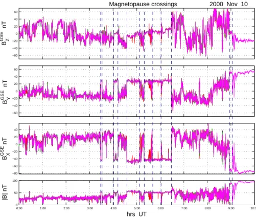
The first encounters of the Cluster spacecraft with the mag-netopause and traversal into the magnetosheath, on 9 and 10 November, followed the arrival of an intense CME at the Earth. This event resulted from the onset of a solar storm two days earlier the details of which are reported elsewhere (Boralv et al., 2001). Although the spacecraft were already in the magnetosheath during the end of 9 November (while at apogee), the sequence of magnetopause encounters occurred on 10 November, as the spacecraft re-entered the magneto-sphere on the southern leg of the orbit. We note that on this day a number of other instruments, including the plasma ion instrument, were not taking data. FGM data from all four Cluster spacecraft are shown in Fig. 1. The data are shown as GSE Cartesian components together with the field mag-nitude, with all spacecraft traces superimposed to highlight any differences in the measured field. In all time series plots, the colour scheme used (here and in the subsequent plots) is: spacecraft 1 (black), 2 (red), 3 (green) and 4 (magenta). It should be noted that a number of commissioning tests were being carried out on spacecraft 1 (black trace) at times dur-ing this day, producdur-ing a number of gaps in the science data. Most of the key magnetopause crossings, however, are cov-ered by continuous data. During normal operation, the in-struments are commanded to provide primary sensor data at 22.4 Hz in the spacecraft normal mode and 67 Hz in the spacecraft burst mode. These data are filtered and re-sampled on board from an internal digital sampling rate of 202 Hz. The magnetometers were operating in normal mode during this day. For illustration here, we have used 1 s averages of the data, but, where appropriate, the boundary analysis has been performed using full resolution data.
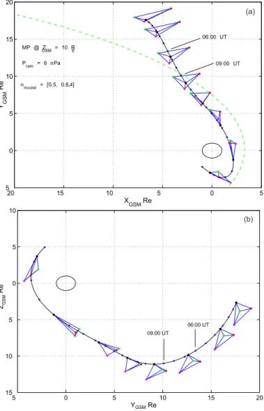
Before discussing the nature of the magnetic field mea-surements in Fig. 1, it is useful to note the spacecraft lo-cation, as shown in Fig. 2. Figure 2a shows a projection
of the inbound leg of the orbit into the X, YGSM plane, for
spacecraft 1, and Fig. 2b shows the corresponding plot for Y ,
ZGSM. The time interval for the whole orbit leg corresponds
to the whole of the day. Each hour is marked by filled circles at intervals along the orbit. Also shown on the orbit are the spacecraft configurations at intervals, projected into the GSM plane. Spacecraft 1 is shown attached to the orbit and the other spacecraft are shown with their corresponding colours in their relative positions at the same time. The size of the spacecraft separation vectors have been scaled up by a factor
of 20 (so that a length on the plot of about 2 REis equivalent
to an actual separation of ∼ 600 km). During the time period of the observations (00:00–09:00 UT), spacecraft 2 and 3 lie almost parallel to the plane of the figure while spacecraft 1 is separated by about 150 km northward and spacecraft 4, about 650 km southward.
In Fig. 1, all spacecraft are therefore located initially near apogee, on the southern leg of the orbit. They lie just south of
the ecliptic plane (X, YGSE), at about 19:00 LT (local time),
and lie in the magnetosheath from the start of the day. Even at apogee, for this orientation of the orbit (see Fig. 2), the
0:00 1:00 2:00 3:00 4:00 5:00 6:00 7:00 8:00 9:00 10:00 0 50 100 |B| nT hrs UT −80 −60 −40 −20 0 20 40 B GSE X nT −60 −40 −20 0 20 40 60 B GSE Y nT −60 −40 −20 0 20 40 60 B GSE Z nT
Magnetopause crossings 2000 Nov 10
Fig. 1. Four-spacecraft, calibrated FGM data taken on 10 November 2000. The data are expressed in GSE coordinates and the field magnitude is given in the bottom panel. The spacecraft traces are represented as individual colours (s/c 1-black, s/c 2-red, s/c 3-green, s/c 4-magenta), but normally these are hidden when the spacecraft see the same field. Inter-spacecraft comparisons show that the calibrated data agree in absolute terms to within ±0.2 nT. Small scale structure, or temporal changes, between the spacecraft appear as deviations between the traces. The spacecraft are in the magnetosheath at the start of the day. An extended encounter with the magnetopause, resulting in a series of crossings (indicated by dashed vertical lines), occurs between 03:30–06:30 UT. Following this, a large compression of the magnetosphere results in an extended period of magnetosheath, followed by a final re-entry into the magnetosphere. The key magnetopause crossings are indicated.
spacecraft would be expected to remain within the
magne-topause for normal solar wind conditions (Pram < 3 nPa).
Thus, the magnetosphere is already somewhat compressed at this time and preliminary solar wind parameters appear to be consistent with this. As the spacecraft traverse the southern leg of the orbit, inbound, they move rapidly south (with
re-spect to GSM coordinates) to about −10 RE at the time of
the final re-entry into the magnetosphere at ∼ 09:00 UT. The spacecraft would therefore be expected to skirt the form of a stationary magnetopause lying just inside the Cluster or-bit. At this local time the magnetospheric field would be ex-pected to be draped substantially tailwards with only a small
BZ component (see discussion below on Fig. 3). At about
03:30 UT, however, the spacecraft re-encounter the magne-topause, which appears to have moved outwards, and begin a sequence of shallow crossings of the boundary layer until 06:30 UT. After 06:30 UT the spacecraft appear to move into deep magnetosheath conditions (see also a companion paper, Lucek et al., this issue).
Preliminary solar wind data (WIND, Acu˜na, et al., 1995) show an extremely large increase in solar wind dynamic
pres-sure, (Pram >20 nPa) at ∼ 06:30 UT (allowing for
convec-tion in the solar wind), behind a strong interplanetary shock.
Although WIND was situated on the dawn side of the Sun-Earth line, this solar wind signature is also seen at Geotail at
about 06:27 UT, located just upstream (∼ 18 RE) of the
mag-netosphere near the sub-solar point. Most ground based in-struments see signatures associated with the magnetospheric compression and subsequent relaxation at ∼ 09:00 UT (Bo-ralv, et al., 2001). We therefore associate the exit of the spacecraft into the magnetosheath at ∼ 06:30 UT with an intense compression of the magnetosphere following arrival of the pressure pulse behind the interplanetary shock. Both the preliminary WIND and Geotail data also indicate that the IMF lies predominantly in the ecliptic, along the Parker
spi-ral direction, or has an unstable BZ(GSE) signature (not
ex-ceeding ∼ 5 nT before the interplanetary shock). The IMF is southward for only brief intervals. In order to obtain an approximate, expected, magnetopause location we only use therefore pressure scaling to fit the magnetopause location (see Dunlop et al., 1999). For simplicity here, we compare magnetopause location to the geometric model of Sibeck et al. (1991). The dashed line shown in Fig. 2a represents a cut of the model magnetopause through the intersection with the orbit (at ∼ 08:55 UT), and corresponds to ∼ 6 nPa, for a cut
20 15 10 5 0 5 5 0 5 10 15 20 YGSM R e XGSM Re MP @ ZGSM = 10 RE Pram = 6 nPa nmodel = [0.5, 0.8, .4] 09:00 UT 06:00 UT (a) 5 0 5 10 15 20 15 10 5 0 5 10 ZGSM R e YGSM Re 06:00 UT 09:00 UT (b)
Fig. 2. (a) Projected plot of the Cluster orbit (spacecraft 1) into X, YGSMcoordinates and model magnetopause location, fitted to the crossing
near 09:00 UT. The configuration of the spacecraft is shown at intervals along the orbit, with the separations scaled by a factor of 20. As can be seen by Fig. 2b, spacecraft 2 and 3 lie almost parallel to the X, Y plane, with spacecraft 1 above and spacecraft 4 below. The magnetopause is shown as a cut through the intersection with the orbit. The model normal and the ram pressure used is also shown (b) As for Fig. 2a, but in the Y , ZGSMplane.
pressure at the sub-solar point remains somewhat higher than this (in excess of 15 nPa) just after 09:00 UT, suggesting that not all the solar wind pressure is transmitted to these high, southern latitudes. The figure also indicates the model nor-mal at the crossing position.
Locating the magnetopause just outside of (or at) the spacecraft positions between 03:30–06:30 UT corresponds to a solar wind dynamic pressure of 4–5 nPa, which is close to that observed at the sub-solar point by Geotail prior to the arrival of the pressure pulse at the interplanetary shock.
The effect of the IMF-BZon the shape of the magnetopause
at this local time and latitude of Cluster is not well known, since most data sets have used available data predominantly from low-latitude spacecraft. Studies of the shape and loca-tion of the magnetopause boundary, including the effect of
IMF-BZ, have been reviewed by Fairfield (1995) and Shue
et al. (2000). Since we use the model boundary for guidance only, a detailed consideration of this effect is not critical to
the discussion here. The effect of a 5 nT IMF-BZon the
flar-ing of the magnetopause on the flanks could be of order 1 RE
(Shue et al., 1998) and this is included in the pressure uncer-tainty quoted above (∼ 1 nPa). After the arrival of the
inter-planetary shock, the IMF-BZ fluctuations increase slightly
but predominantly remaining within ±10 nT, as often north-ward as southnorth-ward. The effect of magnetopause shape on the model normal is much smaller than the deviations in actual normals quoted below.
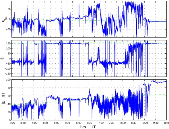
Figure 3 shows the time period containing both the main boundary layer encounter and the final entry into the magne-tosphere, in polar GSE coordinates, for the data from space-craft 4. The T89 magnetospheric field model (Tsyganenko, 1989), corresponding to the high activity conditions observed
3:000 3:30 4:00 4:30 5:00 5:30 6:00 6:30 7:00 7:30 8:00 8:30 9:00 9:30 10:00 20 40 60 80 100 hrs UT |B| nT −150 −100 −50 0 50 100 150 φ −50 0 50 θ lat
Fig. 3. Plot of the magnetic field measured on spacecraft 4 in GSE polar coordinates. The model field, computed using the Tsganenko-89 model for an extreme activity level (KP = 6), is shown as dashed lines. The measured field shows high compression after the 09:00 UT
crossing. The orientation of the model field fits the data very well, except just before the 06:30 UT crossing.
during this event has been added for comparison. The high
KP =6 value corresponds to the best fit to the field
orien-tation, defined by the polar angles, during this data interval. Clearly, the high magnetic field magnitude after 09:00 UT, in comparison to the model field, represents a highly com-pressed magnetosphere and is consistent with there having been a sustained, large increase in solar wind dynamic pres-sure after 06:30 UT. When the spacecraft are measuring mag-netospheric field (for the intervals we identify), the field lies close to themodel field (dashed line) throughout each inter-val. This direction corresponds to a twisted field configu-ration at the southern, night-side location, where the field di-rection points predominantly tailward in a draped orientation. Although the magnetospheric field directions near the mag-netopause follow the model closely, high values of magnetic field intensity are not modelled closely by the T89 model in the flank regions. By contrast, the magnetosheath field shows a variation broadly in line with preliminary IMF behaviour at the WIND spacecraft. After about 02:30 UT it shows a variable north/south orientation, predominantly close to the
Parker spiral (with BXpositive) and this results in high
mag-netic shear across the magnetopause for the crossings be-tween 03:30–06:30 UT. After about 08:00 UT the magne-tosheath field turns predominantly northward, corresponding to the IMF, and away from the Parker spiral direction just be-fore the last crossing. This change in orientation significantly
reduces the local shear across the magnetopause for the last encounter (at 08:55 UT).
3 Magnetopause encounters
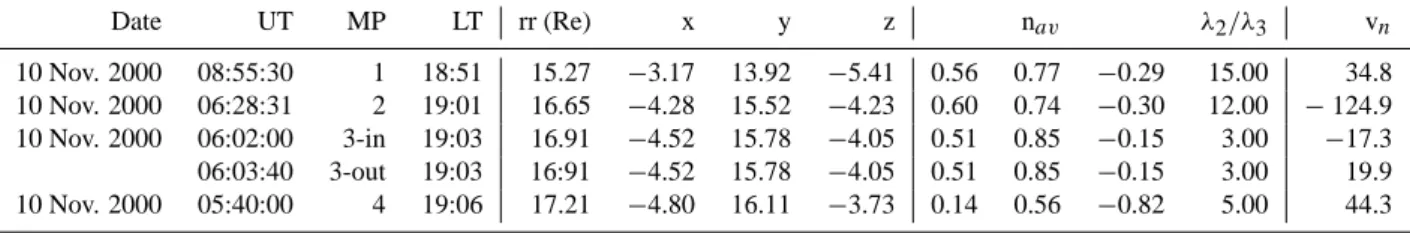
In order to investigate the character of the magnetopause and its dynamics in response to the changing conditions, we se-lect four encounters with the magnetopause. The results of MVA (minimum variance analysis, (Sonnerup and Cahill, 1967)) of each crossing are shown in Table 1. The table shows the date and key time of each crossing, the orbital po-sition of spacecraft 1, the mean boundary normals for each crossing and the mean velocity of the boundary along the normal. The column headed ‘MP’ labels each encounter 1–4, numbered backwards in time. In the Table, we have shown only the average over the individual spacecraft nor-mals and the average of the magnetopause velocity between each spacecraft pair. The velocity is calculated from the in-dividual crossing times at each spacecraft and the projected separation vector for each pair of spacecraft (see Bauer et al., 2000, for an application of inter-spacecraft timing methods using AMPTE IRM/UKS data). We comment on the differ-ences between each spacecraft for the individual crossings below.
Table 1. Boundary analysis results Date UT MP LT rr (Re) x y z nav λ2/λ3 vn 10 Nov. 2000 08:55:30 1 18:51 15.27 −3.17 13.92 −5.41 0.56 0.77 −0.29 15.00 34.8 10 Nov. 2000 06:28:31 2 19:01 16.65 −4.28 15.52 −4.23 0.60 0.74 −0.30 12.00 −124.9 10 Nov. 2000 06:02:00 3-in 19:03 16.91 −4.52 15.78 −4.05 0.51 0.85 −0.15 3.00 −17.3 06:03:40 3-out 19:03 16:91 −4.52 15.78 −4.05 0.51 0.85 −0.15 3.00 19.9 10 Nov. 2000 05:40:00 4 19:06 17.21 −4.80 16.11 −3.73 0.14 0.56 −0.82 5.00 44.3
Although there are small changes in magnetopause orien-tation between encounters, the normals are broadly consis-tent (they agree to within a few percent in direction) and, except for the encounter at 05:25–05:40 UT, are in line with the model magnetopause at each location. Except for the fast crossing at ∼ 06:30 UT (see below), the normals are all stable (to choice of analysis interval), typically with high eigenvalue ratios (> 5) between intermediate and minimum eigenvalues. Statistical errors (as defined in Sonnerup and Scheible, 1998) are small. The evolution of the boundary ori-entation follows the slow change in spacecraft location and the individual boundary normals at each spacecraft show that the local boundary shape has a high degree of planarity. This fact makes the interpretation of each crossing sequence rel-atively easy. In the majority of cases, repeated encounters with the magnetopause boundary show nested sequences of crossing times at each spacecraft; strong support for the in-terpretation that the crossings are caused by in/out motion of the boundary, rather than convected structure moving passed the Cluster configuration. Such nested timing is maintained for all crossings throughout the day, although the actual or-der of the spacecraft encounters changes when the boundary orientation changes.
The magnetosheath field remains closely aligned to the magnetopause plane, except for some notable intervals dis-cussed below. This suggests that, at least for the interval 03:30–06:30 UT, the Cluster configuration remains close to the magnetopause and is consistent with small, but chang-ing, motion of the magnetopause during this period. The computed velocities confirm this, noting that we use the con-vention that outward motion of the magnetopause, along the (outward) normal to the boundary, is positive. Crossing 1 oc-curs after the magnetopause has stabilised and is slowly re-expanding, since it shows a clear outward motion at all the spacecraft. The corresponding normal directions at cross-ing 1 are closely aligned to the model normal. The encounter follows the large magnetospheric compression, which oc-curred immediately after crossing 2, where subsequently, the spacecraft moved substantially south with respect to the GSM equator and followed the magnetopause inwards un-til 09:00 UT. Crossing 2 shows a high inward velocity, con-sistent with the onset of a large compression of the magne-topause. Crossing 3 is chosen because it shows a rapid but simple reversal in boundary velocity which corresponds to a similar low speed for both the inwards and outwards motion of the boundary, consistent with a small amplitude
depres-sion of the magnetopause. Crossing 4 is also consistent with outward motion.
Corresponding to the table, each crossing is discussed be-low in more detail, in reverse time order.
3.1 The crossings between 08:30 and 09:00 UT
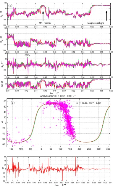
Figure 4a shows the interval around the final re-entry of the Cluster spacecraft into the magnetosphere for all four space-craft. In fact, as shown by Fig. 1, there are more brief cross-ings back into the magnetosheath after 09:00 UT, after which the spacecraft remain in the magnetosphere. Only data from spacecraft 4, however, were recovered for these later times. The data are expressed in MVA coordinates, with ‘N ’ along the minimum variance direction, ‘M’ along the intermedi-ate variance direction and ‘L’ along the maximum variance direction. The coordinates have been determined for each spacecraft separately by performing MVA across the magne-topause. The boundary normals (minimum variance direc-tion) at each spacecraft are, however, closely aligned (within 1%) and are very stable with a high separation of the min-imum and intermediate eigenvalues. The profiles of each spacecraft show a high degree of agreement, but also show evidence of small-scale structure. The gross (low frequency) field configuration around the magnetopause, and the implied planar geometry of the magnetopause, are therefore main-tained on the scale of the spacecraft separations (which range from ∼ 400 to ∼ 1000 km).
The BN component shows fluctuations about zero,
sug-gesting that the magnetic alignment is tangential across the boundary and that the magnetosheath field remains closely
aligned to the magnetopause. This is confirmed by the
boundary analysis. Figure 4b, for instance, shows a scatter plot of the GSE angles of the magnetic field for an interval around the magnetopause. The data are from spacecraft 4 and the MVA normal is quoted on the plot. Two curves are drawn through the points (see Dunlop and Woodward, 1998 and Dunlop et al., 1999 for a description). The green curve represents a fitted planar field geometry (where the magnetic field vector lies in different directions but on a plane) to the points and the red curve the equivalent plane defined by the MVA normal. The two curves agree to within the statistical
error and, together with θbn(the out of plane angle and lower
panel in Fig. 4b), confirm tangential field alignment across the magnetopause. As indicated in Fig. 4a, there is a brief, earlier encounter with the magnetopause, between 08:44:30–
8:380 8:40 8:42 8:44 8:46 8:48 8:50 8:52 8:54 8:56 8:58 9:00 50 100 |B | n T hrs UT 8:38 8:40 8:42 8:44 8:46 8:48 8:50 8:52 8:54 8:56 8:58 9:00 40 20 0 20 40 BN n T 8:38 8:40 8:42 8:44 8:46 8:48 8:50 8:52 8:54 8:56 8:58 9:00 100 50 0 50 100 BM n T 8:38 8:40 8:42 8:44 8:46 8:48 8:50 8:52 8:54 8:56 8:58 9:00 100 50 0 50 100 BL n T Magnetosphere MP reentry FTEs (a) 150 100 50 0 50 100 150 200 250 300 350 80 60 40 20 0 20 40 60 80 la t Analysis interval = 8:42 8:59 UT 8:42 8:43 8:44 8:45 8:46 8:47 8:48 8:49 8:50 8:51 8:52 8:53 8:54 8:55 8:56 8:57 8:58 8:59 9:00 9:01 60 40 20 0 20 40 60 hrs UT bn n = (0.57, 0.77, 0.30) (b)
Fig. 4. (a) Interval of data in minimum variance coordinates around crossing 1, as in Table 1. MVA is performed for each spacecraft separately in order to express the data in LMN coordinates. The interval is chosen to show both the brief re-entry into the magnetosphere and two clear FTE signatures in the magnetosheath. The analysis is performed at high resolution (22.4 Hz). (b) Result of the boundary analysis, as described in the text, where the interval plotted refers to the scatter plot. The MVA was performed across the MP at 08:56 UT.
08:46:30 UT, suggesting that the spacecraft remain adjacent to the magnetopause, but in the magnetosheath, around this time. The traces show a larger time delay at 08:44:30 UT than at 08:46:30 UT. Since the normal direction does not change for the inbound or outbound crossing, the nested sig-nature of the re-entry (most clear for the red trace), therefore, indicates a slower entry into the magnetospheric boundary, than the exit. Note that throughout the plot, the black and green traces remain close together, reflecting the fact that these two spacecraft (1 and 3) remain closely parallel to the magnetopause plane. There are a number of short turnings
in the BN component throughout the period shown but two
strong, bipolar signatures with FTE-like signatures (Russell and Elphic, 1979) are notable at 08:39:15 and 08:42:20 UT. These signatures stand out because of the similarity at each
spacecraft (which sets the overall scale size to be of order 1000 km, or greater) and their close coincidence in time. At high resolution, the time shifts between each spacecraft trace suggest a convection speed of 700–900 km/s, parallel to the magnetopause and a corresponding scale (along the flow) over the signature of 4000–5000 km. This is consistent with the expected magnetosheath flow for the solar wind condi-tions at this time. In detail, there is structure on the space-craft separation scale, particularly within the enhancements in field strength. At high time-resolution, for the first event (at 08:39:15 UT), spacecraft 1 and 3 both show a dip in |B| in the centre of the event, while spacecraft 2 and 4 do not (not clear from Fig. 4a). As referred to above, the orientation of the magnetopause is such that spacecraft 1 and 3 lie almost parallel to its plane, with spacecraft 2 and 4 lying further out
6:18 6:19 6:20 6:21 6:22 6:23 6:24 6:25 6:26 6:27 6:28 6:29 6:30 6:31 6:32 6:33 6:34 40 60 80 |B | n T hrs UT 6:18 6:19 6:20 6:21 6:22 6:23 6:24 6:25 6:26 6:27 6:28 6:29 6:30 6:31 6:32 6:33 6:34 40 20 0 20 BN n T 6:18 6:19 6:20 6:21 6:22 6:23 6:24 6:25 6:26 6:27 6:28 6:29 6:30 6:31 6:32 6:33 6:34 80 60 40 20 0 20 40 60 BM n T 6:18 6:19 6:20 6:21 6:22 6:23 6:24 6:25 6:26 6:27 6:28 6:29 6:30 6:31 6:32 6:33 6:34 60 40 20 0 20 40 60 BL n T Magnetosphere Magnetosheath
Partial exit or wave
(a) 150 100 50 0 50 100 150 200 250 300 350 80 60 40 20 0 20 40 60 80 la t Analysis interval = 6:26 6:30 UT 6:26:00 26:30 27:00 27:30 28:00 28:30 29:00 29:30 30:00 50 40 30 20 10 0 10 bn mins UT n = (0.62, 0.57, 0.54) (b)
Fig. 5. (a) As for Fig. 4a, but for crossing 2. (b) As for Fig. 4b, but for crossing 2. The planar fit to the scatter plot is not shown.
(spacecraft 4 is also south of the others). For a cylindrical flux tube moving along the magnetosheath flow, therefore, spacecraft 1 and 3 would cut through the structure similarly. At the magnetopause crossing at 08:56 UT, it is clear from
the BLcomponent that spacecraft 1 and 3 pass through the
magnetic shear almost at the same time, followed by space-craft 4 and then spacespace-craft 2 (a similar sequence occurs at the brief entry at 08:44:30 UT). The nature of this crossing at all the spacecraft is consistent with the view that the mag-netosphere is undergoing expansion and recovery, following the large compression earlier. Using the independently de-termined normals, which demonstrate a high degree of pla-narity over the spacecraft tetrahedron, we can compute pro-jected speeds along the normals for each spacecraft pair from the inter-spacecraft timing and separation vectors. We do not describe the full technique here, since it is described else-where in detail but it is worth noting the following points. The calculation rests on each spacecraft measuring similar
substructure, which produces stationary features in the time-series. Since, in general, significant intervals of data around the boundary will contain features representing both time de-pendence and spatial structure, this means that the use of correlation techniques for the timing usually fail. Moreover, constant velocity can almost never be assumed. Although the boundary here is relatively stable, we find that the veloc-ity changes smoothly from 20 km/s to 45 km/s as it passes the spacecraft array. We estimate that the boundary layer extends over about 30 s, giving a thickness of ∼ 1000 km, corresponding to the mean speed in Table 1.
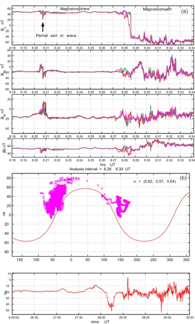
3.2 The crossings at 06:30 UT
Figure 5a shows an overview of the magnetopause crossing at the time of arrival of the interplanetary shock and increase in solar wind dynamic pressure in the same format as for Fig. 4a. At a convection speed of up to 900 km/s, the pressure
increase could arrive at Cluster just before the crossing while the spacecraft were still in the magnetosphere. The main characteristic of this crossing is the speed of traversal, which results in almost simultaneous exit times at spacecraft 1, 3 and 4. There is also significant structure (on the scale of the spacecraft separation) within the magnetospheric bound-ary layer (06:27:50–06:28:40 UT) and the separation of the red trace for spacecraft 2 suggests rapid acceleration between this and the other spacecraft.
MVA analysis of the boundary and adjacent region gives the normals, quoted in Table 1, which are consistent with the model normals at this position and all spacecraft agree to within 5%. However, the complexity of the magnetopause
layer itself, which appears to contain an embedded FTE (BN
signature) or boundary wave, produces slightly different
nor-mals. The traces for BN, in Fig. 5a, show deviations
be-tween the spacecraft, but all have a consistent component of
∼ 20 nT, indicating that the current layer has the form of a
rotational discontinuity. Figure 5b shows the high-resolution analysis for spacecraft 3 in the format of Fig. 4b. The evi-dence from the scatter plot suggests that the underlying
mag-netopause plane has a much smaller ZGSE component than
suggested by the MVA normal. Such an orientation places the magnetopause almost parallel to the spacecraft plane de-fined by spacecraft 1, 3 and 4. Spacecraft 2 lies almost per-pendicular to this plane at a separation of about 650 km. Such a local orientation of the magnetopause would be consistent with a sudden large compression, driving the magnetopause inwards.
Although this alignment of the spacecraft and magne-topause planes means that the computed speed of the bound-ary is sensitive to the normal direction, the mean velocity from the spacecraft 2 timing can be accurately found and is 45 km/s. Moreover, the only consistent analysis of the motion suggests that the boundary speed increases to over 300 km/s at spacecraft 1 so that there is a rapid acceleration of the magnetopause inwards. It is again true that space-craft 1 and 3 sample very similar fields, while spacespace-craft 2 shows distinct structure. Spacecraft 4 shows almost the same profile as that for 1 and 3 after 08:28:35 UT, corresponding to the outer current layer and in line with the boundary ori-entation implied above. Spacecraft 2 sees different structure through the boundary and transition layers, but all spacecraft show signatures that are consistent with a high shear bound-ary (Paschmann et al., 1986; Phan et al., 1994). The transi-tion layer again extends over 30 s and the perpendicular scale of the boundary layer at the velocity determined from space-craft 2 is, therefore, again just larger than ∼ 1000 km.
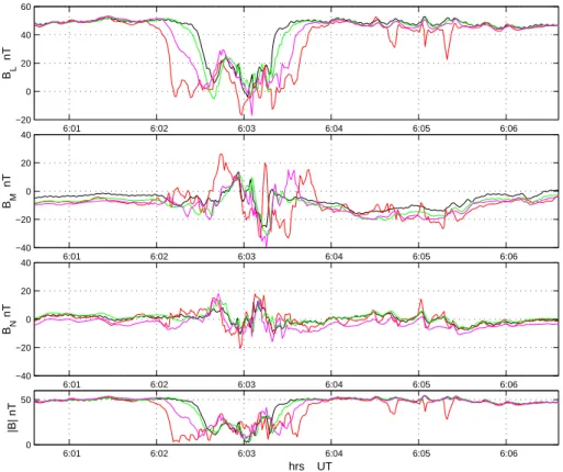
3.3 The crossings at 06:05–06:10 UT
Figure 6 shows a pair of magnetopause crossings correspond-ing to a simple reversal in magnetopause motion (as indicated in Table 1). The magnetopause structure is almost the same for both the inward and outward crossing, so that the field profiles are reversed around 06:03 UT. The MVA normals are not so well determined for this interval, but show a slight
rotation into YGSE. Small differences between the spacecraft
are within statistical error. The twin bipolar signature on the magnetosheath side of the boundary is similar to that seen in the magnetospheric layer and appears to be a standing struc-ture with little or no time shift between the signastruc-tures. Again spacecraft 1 and 3 show similar profiles which would align the structure to the magnetosheath field (primarily along the Parker spiral). There are a number of magnetospheric FTE signatures after 06:04 UT (see below).
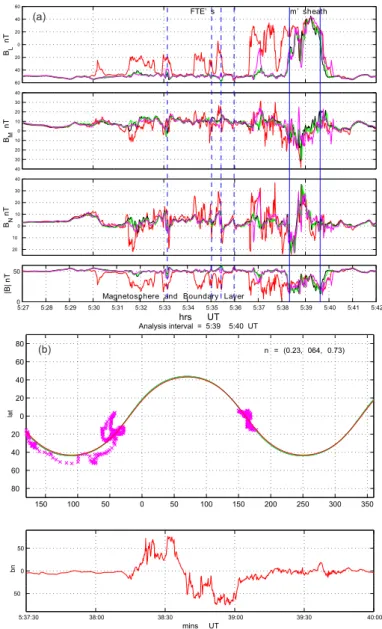
3.4 The crossings at 05:40 UT
Figure 7a shows a magnetopause encounter for which the spacecraft remain in or very near the boundary for more than ten minutes. All spacecraft exit briefly into the mag-netosheath between 05:38 and 05:40 UT; and then all return into the magnetosphere as the magnetopause moves outwards for a sustained period. The MVA analysis was performed on the final set of crossings and produced stable normals to a tangential boundary (at least on the magnetospheric side), as can be seen in Fig. 7b for spacecraft 3. All normals for each spacecraft were again closely aligned (< 1%). It is appar-ent that the magnetopause oriappar-entation differs from the model normal and, from the later encounters, tilting predominantly
into YGSE and ZGSE. This affects the crossing order for the
spacecraft so that spacecraft 2 is no longer perpendicular to the boundary. The magnetospheric and magnetosheath fields have the same orientation and still see very similar field pro-files. Spacecraft 4, however, now has a larger separation along the normal.
On exit, however, at 05:38:15 UT, the magnetopause ori-entation is consistent with the model normals, so that space-craft 2 is still the outer most spacespace-craft relative to the bound-ary orientation, showing multiple crossings of the magne-topause throughout the earlier period while the other space-craft remain predominantly on the magnetospheric side of the boundary. During this interval (05:30–05:38 UT), there-fore, the magnetopause boundary layer lies sometimes be-tween spacecraft 2 and the other spacecraft and, on at least one occasion spacecraft 4 makes a partial exit into the netosheath. Spacecraft 1 and 3 always lie deeper on the
mag-netospheric side of the boundary. The BNtrace shows close
alignment to the magnetopause orientation and contains a number of (magnetospheric) FTE signatures. We have in-dicated four by dashed vertical lines. In some cases, notably the signatures at 05:35:00 and 05:35:25 UT, the same coher-ent signature is observed even when spacecraft 2 is in the magnetosheath. Thus, the same reconnected flux is seen on either side of the current layer. In the second case, for ex-ample, spacecraft 4 passes through the centre of the flux tube while the others lie either side of the boundary.
Spacecraft 2 is only 400 km from spacecraft 4, along the normal, and the other spacecraft are less than 200 km sep-arated so the FTE signature represents a structure of order or less than the scale of the overall boundary layer. This is consistent with previous studies of ISEE 1 and 2. Moreover, these magnetospheric signatures are of short duration,
6:01 6:02 6:03 6:04 6:05 6:06 0 50 |B| nT hrs UT 6:01 6:02 6:03 6:04 6:05 6:06 −40 −20 0 20 40 BN nT 6:01 6:02 6:03 6:04 6:05 6:06 −40 −20 0 20 40 BM nT 6:01 6:02 6:03 6:04 6:05 6:06 −20 0 20 40 60 BL nT
Fig. 6. As for Fig. 4a, but for crossing 3.
ing a speed along the magnetopause of ∼ 20 − 80 km/s, from previous estimates of their spatial scale. There is also an
im-plication for the size of the BN perturbation, which appears
to be always larger on the magnetosheath side of the bound-ary. This is true for the FTE’s seen at 06:05 UT also (see Fig. 6). It is expected that the size of the signature should grow as the spacecraft cut closer to the current layer and that deeper into the magnetosphere the signature weakens.
4 Conclusions
We have discussed the four spacecraft magnetic field data from the Cluster mission for the first day of crossings of the magnetopause by spacecraft . We have focussed on four dis-tinct encounters, each with particular characteristics, but in the context of the magnetospheric conditions applying to the whole day. The two main intervals of magnetospheric field, before and after the arrival of the interplanetary shock, also have associated ground signatures which, are discussed else-where (this issue). The whole set of crossings, measured si-multaneously at the four spacecraft, in general result in a se-quence of crossing times which is consistent in all cases with large scale (but often small amplitude) motions of the mag-netopause. The individual ordering, in which the spacecraft cross the boundary at each crossing, and indeed the timing of other comparative features in the field profiles, have to be un-derstood in terms of the orientation of the magnetopause with respect to the spacecraft configuration. For this event, it is
demonstrated, by direct application of MVA across the mag-netopause, that the geometry of the magnetopause is highly planar over the spacecraft array. The mean magnetopause orientation changes slowly over the day and is observed to change the crossing order of the spacecraft. A planar config-uration makes inter-comparison of the magnetic field signa-tures more straightforward but also allows the motions of the magnetopause to be determined unambiguously for the first time.
We have been able to show that in nearly all cases the mag-netopause motion is constantly changing and in particular varies over the sequence of spacecraft crossing times. Mag-netopause speeds along the normal for the sequence of in/out crossings between 03:30–06:30 UT range from 17–44 km/s; the arrival of a pressure pulse of more than 20 nPa produced magnetopause speeds of over 300 km/s. On the scale size of the Cluster separation distances, here ranging from 200– 650 km for the whole time interval, the magnetopause ve-locity is hardly ever constant. It is also demonstrated that the particular geometry for this day resulted in the magnetopause lying nearly planar to one face of the spacecraft tetrahedron, so that the inter-spacecraft timing is sensitive to changes in magnetopause orientation.
The scale size of the magnetopause layer was shown to be consistently (for different crossing speeds) about 1000– 1100 km. It is important to note that, in the presence of strong sudden accelerations, an assumption of constant mo-tion over these spatial scales (as has to be done in the case of dual spacecraft measurements) would falsely estimate the
5:270 5:28 5:29 5:30 5:31 5:32 5:33 5:34 5:35 5:36 5:37 5:38 5:39 5:40 5:41 5:42 50 |B | n T hrs UT 20 10 0 10 20 30 40 BN n T 40 30 20 10 0 10 20 30 40 BM n T 60 40 20 0 20 40 60 BL n T
Magnetosphere and Boundary Layer
m’ sheath FTE’ s (a) 150 100 50 0 50 100 150 200 250 300 350 80 60 40 20 0 20 40 60 80 la t Analysis interval = 5:39 5:40 UT 5:37:30 38:00 38:30 39:00 39:30 40:00 50 0 50 bn mins UT n = (0.23, 064, 0.73) (b)
Fig. 7. (a) As for Fig. 4a but for crossing 4. The interval is chosen to correspond to the extended sequence of multiple crossings by spacecraft 2. The dashed vertical lines indicate selected FTE signatures and the short period when all spacecraft exit into the magnetosheath is shown by solid vertical lines. (b) Analysis of the boundary at 05:40 UT.
boundary thickness. Such an estimate would vary, depend-ing on the changes in motion of the boundary. Correct use of four spacecraft information can determine, as is done here, what changes in motion occur. The perpendicular scale of embedded structures, such as FTE’s, was shown to be of or-der or less than the magnetopause thickness. In the adjacent magnetosheath, a number of candidate FTE signatures were observed and two convected signatures, seen after the large solar wind pressure pulse, were shown to imply a magne-tosheath speed of ∼ 800–1000 km/s, consistent with the solar wind speed.
For significant time intervals, the spacecraft array re-mained near, in, or across both the magnetosheath and mag-netopause boundary layers. On a number of occasions, FTE signatures were observed by different spacecraft on either side of the magnetopause current layer. There is clear
evi-dence that the scale of the signature is largest on the mag-netosheath side of the boundary and has some variation with distance from the boundary. The implied flux tube motion of ∼ 100 km/s along the magnetopause boundary suggests a parallel scale of ∼ 0.5 RE.
Acknowledgements. This work was supported at Imperial College by PPARC. Comments on the up-stream solar wind conditions were made on the basis of key parameter data held at the NASA/GSFC Space Physics Data Facility and the NSSDC, obtained via CDAweb. WIND data is made available by K. Ogilvie and R. Lepping. Geo-tail data is made available by L. Frank and S. Kokubun.
Topical Editor G. Chanteur thanks J. L. Burch and another ref-eree for their help in evaluating this paper.
References
Acu˜na, M., Ogilvie, K. W., Baker, D. N., Curtis, S. A., Fairfield, D. H., and Mish, W. H.: The global Geospace program and its investigations, Space Sci. Rev., 71, 5, 1995.
Balogh, A., Carr, C. M., Acu˜na, M. H., Dunlop, M. W., Beek, T. J., Brown, P., Fornac¸on, K.-H., Georgescu, E., Glassmeier, K.-H., Harris, J., Musmann, G., Oddy, T., and Schwingenschuh, K.: The Cluster magnetic field investigation: overview of in-flight perfor-mance and initial results, Ann. Geophysicae, this issue, 2001. Balogh, A., Cowley, S. W. H., Dunlop M. W., et al.: The
Clus-ter magnetic field investigation: Scientific objectives and instru-mentation, in Cluster: mission, payload and supporting activities, ESA SP-1159, 95, 1993.
Balogh, A., Dunlop, M. W., et al.: The Cluster magnetic field inves-tigation, Space Science Reviews, 79, 65, 1997.
Bauer, T. M., Dunlop, M. W., Sonnerup, B. U. ¨O, Sckopke, N., Fazakerley, A. N., and Khrabrov, A. V.: Duel spacecraft determi-nations of magnetopause motion, Geophys. Res. Lett., 27, 1835– 1838, 2000.
Berchem, J. and Russell, C. T.: The thickness of the magnetopause current layer: ISEE 1 and 2 observations, J. Geophys. Res., 87, 2108–2114, 1982.
Bor¨alv, E., Donovan, E., Voronkov, I., Eglitis, P., Amm, O., Andr´e, M., Balogh, A., Behlke, R., Cowley, S. W. H., and Dunlop, M., W.: The Storm of 10 November 2000, submitted to, J. Geophys. Res., 2001.
Bryant, D. A., Krimigis, S. M., and Haerendel, G.: Outline of the Active Magnetospheric Particle Tracer Explorers (AMPTE) mis-sion, IEEE Trans. Geosci. Remote Sensing, GE-23, 177, 1985. Dunlop, M. W., Balogh, A., Baumjohann, W., Haerendel, G.,
Fornac¸on, K.-H., Georgescu, E., et al.: Dynamics and local boundary properties of the dawn-side magnetopause under con-ditions observed by equators, Ann. Geophysicae, 17, 1535–1559, 1999.
Dunlop, M. W. and Woodward, T. I.: Discontinuity analysis: ori-entation and motion, in: Analysis methods for multispacecraft data, ISSI Scientific Report SR-001, ESA Publications, Noord-wijk, The Netherlands, p. 271, 1998.
Elphic, R. C.: Multipoint observations of the magnetopause: results from ISEE and AMPTE, Adv. Space Res., 8, 223–238, 1988. Elphic, R. C.: Observations of flux transfer events: are FTE’s flux
ropes, islands, or surface waves?, in: Physics of the Magnetic Flux Ropes, (Eds) Song, Russell et al., AGU Geophysical Mono-graph 58, 455–471, 1990.
Elphic, R. C.: Observations of flux transfer events: a review, in: Physics of the Magnetopause, (Eds) Song, Sonnerup and Thompsen, AGU Geophysical Monograph 90, 225–233, 1995. Fairfield, D. H.: Shape and location of the magnetopause, in Physics
of the Magnetopause, (Eds) Song, Sonnerup and Thompsen, AGU Geophysical Monograph 90, 115–122, 1995.
Lucek, E. A., Dunlop, M. W., Horbury, T., Balogh, A., Cargill P., and the FGM team: Cluster magnetic field observations in the magnetosheath, Ann. Geophysicae, this issue, 2001.
Paschmann, G., Papamastorakis, I., Baumjohann, W., Sckopke, N., Carlson, C. W., Sonnerup, B. U. ¨O., and L¨uhr, H.: ISEE ob-servations of the magnetopause: Reconnection and the energy balance, J. Geophys. Res., 90, 12 111–12 120, 1985.
Paschmann, G., Papamastorakis, I., Baumjohann, W., Sckopke, N., Carlson, C. W., Sonnerup, B. U. ¨O., and L¨uhr, H.: The Magne-topause for large magnetic shear: AMPTE/IRM observations, J. Geophys. Res., 91, 11 099–11 115, 1986.
Phan, T.-D., Paschmann, G., Baumjohann, W., Sckopke, N., and L¨uhr, H.: The magnetosheath region adjacent to the dayside mag-netopause: AMPTE/IRM observations, J. Geophys. Res., 99, 121–141, 1994.
Phan, T.-D. and Paschmann, G.: The magnetosheath region adja-cent to the dayside magnetopause, in: Physics of the Magne-topause, (Eds) Song, Sonnerup and Thompsen, AGU Geophysi-cal Monograph 90, 115–122, 1995.
Russell, C. T.: The structure of the magnetopause, in: Physics of the Magnetopause, (Eds) Song, Sonnerup and Thompsen, AGU Geophysical Monograph 90, 81–98, 1995.
Russell, C. T. and Elphic, R. C.: Initial ISEE magnetometer results: Magnetopause observations, Space Sci. Rev., 22, 681–715, 1978. Russell, C. T. and Elphic, R. C.: ISEE observations of flux transfer events at the dayside magnetopause, Geophys. Res. Lett., 6, 33– 36, 1979.
Shue, J. -H., Song, P., Russell, C. T., Steinberg, J. T., Chao, J. K., Zastenker, G., Vaisberg, O. L., Kokubun, S., Singer, H. J., and Detman, T. R.: Magnetopause location under extreme solar wind conditions, J. Geophys. Res., 103, 17, 691, 1998.
Shue, J. -H., Song, P., Russell, C. T., Chao, J. K., and Yang, Y. H.: Toward predicting the position of the magnetopause within Geosynchronous orbit, J. Geophys. Res., 103, 17, 691, 2000. Sibeck, D. G., Lopez R. E., and Roelof, E. C.: Solar wind control of
the magnetopause shape location and motion, J. Geophys. Res., 96, 5489, 1991.
Sonnerup, B. U. ¨O. and Cahill, L. J.: Magnetopause structure and attitude from Explorer 12 observations, J. Geophys. Res., 72, 171–183, 1967.
Sonnerup, B. U. ¨O. and Scheible, M.: ‘Maximum and minimum variance analysis’, in: Analysis Methods for Multispacecraft Data, ISSI Science Report, SR-001, Kluwer Academic Pub., 1998.
Tsyganenko N. A.: A magnetospheric field model with a warped tail current sheet, Planet. Space Sci., 37, 1, 5–20, 1989.