Segmentation of pelvic structures for planning CT using a geometrical shape model tuned by a multi-scale edge detector.

HAL Id: inserm-00959273

https://www.hal.inserm.fr/inserm-00959273

Submitted on 4 Oct 2014

HAL is a multi-disciplinary open access

archive for the deposit and dissemination of sci-entific research documents, whether they are pub-lished or not. The documents may come from teaching and research institutions in France or abroad, or from public or private research centers.

L’archive ouverte pluridisciplinaire HAL, est destinée au dépôt et à la diffusion de documents scientifiques de niveau recherche, publiés ou non, émanant des établissements d’enseignement et de recherche français ou étrangers, des laboratoires publics ou privés.

a geometrical shape model tuned by a multi-scale edge

detector.

Fabio Martínez, Eduardo Romero, Gaël Dréan, Antoine Simon, Pascal

Haigron, Renaud de Crevoisier, Oscar Acosta

To cite this version:

Fabio Martínez, Eduardo Romero, Gaël Dréan, Antoine Simon, Pascal Haigron, et al.. Segmentation of pelvic structures for planning CT using a geometrical shape model tuned by a multi-scale edge de-tector.. Physics in Medicine and Biology, IOP Publishing, 2014, 59 (6), pp.1471-1484. �10.1088/0031-9155/59/6/1471�. �inserm-00959273�

geometrical shape model tuned by a multiscale edge detector

CIM&Lab, Universidad Nacional de Colombia, Bogota, Colombia

2

INSERM, U1099, Rennes, F-35000, France

3

Université de Rennes 1, LTSI, Rennes, F-35000, France

4

Département de Radiothérapie, Centre Eugène Marquis, Rennes, F-35000, France E-mail: edromero@unal.edu.co

Abstract. Accurate segmentation of the prostate and organs at risk in computed tomography (CT) images is a crucial step for radiotherapy (RT) planning. Manual segmentation, as performed nowadays, is a time consuming process and prone to errors due to the a high intra- and inter-expert variability. This paper introduces a new automatic method for prostate, rectum and bladder segmentation in planning CT using a geometrical shape model under a Bayesian framework. A set of prior organ shapes are first built by applying Principal Component Analysis (PCA) to a population of manually delineated CT images. Then, for a given individual, the most similar shape is obtained by mapping a set of multi-scale edge observations to the space of organs with a customized likelihood function. Finally, the selected shape is locally deformed to adjust the edges of each organ. Experiments were performed with real data from a population of 116 patients treated for prostate cancer. The data set was split in training and test groups, with 30 and 86 patients, respectively. Results show that the method produces competitive segmentations w.r.t standard methods (Averaged Dice = 0.91 for prostate, 0.94 for bladder, 0.89 for Rectum) and outperforms the majority-vote multi-atlas approaches (using rigid registration, free-form deformation (FFD) and the demons algorithm)

Keywords: CT segmentation, Radiotherapy planning, Prostate cancer, Bayesian models, geometrical multiscale descriptors

1. Introduction

Prostate cancer is one of the most commonly diagnosed male cancer worldwide, with190.000 new cases diagnosed in USA in 2010 (American Cancer Society) and 71.000 new cases in France in 2011 (INCa 2011). External beam radiation therapy (EBRT) is a commonly prescribed treatment for prostate cancer which has proven to be efficient for tumor control [1]. EBRT uses high energy beams from multiple directions in order to deliver the dose within the patient tumor region to destroy the cancer cells. Modern treatment techniques offer nowadays improved treatment accuracy through a better planning, delivery, visualization and the correction of patient setup errors. Segmentation plays a major role during the whole therapy. During a standard protocol for EBRT planning, CT images are manually delineated to define not only the clinical target volume (CTV), prostate and seminal vesicles, but also the neighbouring organs at risk (OARs), for instance the bladder and rectum. The CTV is then expanded to constitute the Planning Target Volume (PTV) for treatment. These spatial margins between the organs and the PTV as depicted in Figure 1 allow for uncertainties in delineation, patient setup, motion and organ deformations [23, 12]. The segmentation allows the definition of dose constraints according to a certain recommendations. The International Commission on Radiation Units and Measurements (ICRU) 50 and 62 reports, for example, define and describe several target and critical structure volumes that aid in the treatment planning process and may provide a basis for comparison of treatment outcomes. Thus the directions, strengths, and shapes of the treatment beams are computed in a planning platform to comply with them, following a particular dose prescription. The delineated structures may also be used in further stages and with different purposes during the treatment such as the computation of cumulated dose when image guided radiotherapy (IGRT) is used or for toxicity population studies [9, 17, 4].

In current radiotherapy planning, the CT is still used to perform the segmentation since the dose computation relies on the CT electron density information. However, the CT offers a poor soft tissue contrast and therefore segmenting pelvic organs is highly time consuming (between 20-40 minutes to delineate each), and prone to errors, especially in the apical and basis regions [18]. Previous studies have reported variations in prostate delineation of about 20.60 % of the organ volume [22]. These uncertainties lead to large intra- and inter-observer variabilities and may impact the treatment planning [19] and dosimetry [11, 5]. Hence, reliable, efficient and reproducible (semi)-automatic segmentation techniques are are required in treatment planning.

Several difficulties hamper automatic segmentation methods in this context: (i) the poor border contrast between adjacent organs, (ii) the high intra- and inter-individual shape variability, (iii) the inhomogeneities in the amount of bladder and rectum filling [20] (iv) the often presence of fiducial markers used to guide dose delivery. Common automatic methods for organ segmentation of pelvic structures include deformable models [15, 35], atlas based methods [39] or statistical shape models [3, 33]. Atlas based approaches use prior learning not only for obtaining a final contour but also to provide initial organ positions for further segmentation algorithms. In atlas-based methods a pre-computed segmentation

or prior information (i.e. probability map) in a template space is propagated to the image to be segmented via registration [36, 2, 39, 26]. Although atlas-based approaches may provide prior structural information, a high inter-individual variability and registration errors may lead this method to fail. Multi-atlas approaches can partly overcome some of these difficulties by selecting the most similar organ of interest among a large database, but the definition of a proper similarity metrics between the available atlases and the individual query, is still an open issue [39, 47, 39]. Statistical shape models may help to overcome atlas-based segmentation problems by introducing prior shapes, which in a further step may be locally adjusted [3, 33]. In general, these approaches define a cost function encoding similarities that matches a prior shape/appearance knowledge with a particular individual (test image) [40, 34]. These approaches are relatively stable and robust to noise and voxel variations, however their accuracy may be limited by the set of features selected to represent the image test and the particular definition of the match function. Examples of prostate segmentation following this approach appear in [32] where the segmentation problem was addressed without shape constraints by allowing flexibility to individual local variations, with some issues, however, in regions with poor contrast. More recently, Che et al [25] proposed a statistical method that matches the prior shape information under a Bayesian hypothesis, incorporating anatomical constraints but without exploiting spatial information. Other approaches include learning strategies to segment the prostate, but within the context of intra-individual segmentations where previous organ delineations are required [27].

In this paper, we propose a novel method for automatically segmenting pelvic structures from CT scans based on a statistical shape model within a Bayesian framework and with local spatial variations. The proposed approach is appropiate for different types of organ, shapes, as well as stable to variations in contrast and bladder and rectum filling conditions. A method for removing CT artifacts was implemented which increases contours reliability using an adapted non-local filter, which was able to overcome the issues with fiducial markers. Since the prior is built from different available shapes, the approach is robust to the large inter-individual variability. The likelihood matching includes a geometrical and topological analysis which allows to set an optimal correspondence between a prior 3D shape model and the considered CT. Such prior is built from an actual population while a multi-scale edge descriptor allows for the mapping between the prior and the CT observations. The yielded 3D organ segmentation is spatially coherent and voxels are connected together. In the remainder of this paper we first describe the method, we then validate the accuracy of our approach on real CT data, and compared with baseline Atlas-Based segmentation methods.

.

2. Methodology

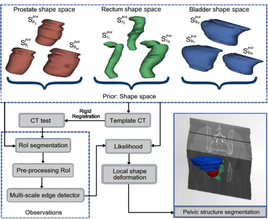
The proposed method consists of several stages as depicted in Figure 2. Let bSo, the estimated

(a) (b) (c) (d)

Figure 1. Example of planning dose on manually segmented CT. a) original CT scan, b) prostate and rectum delineations, c) PTV is obtained by adding margins to the prostate and c) Resulting 3D planning dose. The presence of fiducial markers may hamper segmentation.

under a Bayesian framework b So = max c So arg[P ( bSo|Sopca1 , S pca o2 , . . . , S pca oN)] (1) where _{Spca o1 , S pca o2 , . . . , S pca

oN} is a collection of shapes (the shape space) of the organ o.

The reference template serves as the coordinate framework of the PCA geometrical shape model and corresponds simply to a random seletion of a single CT-image. The likelihood function (section 2.4), aimed to match the most similar shape with the observations extracts information from a multi-scale analysis in a RoI around the organs (section 2.3), after removing CT artifacts. Eventually, the most likely shape bSois locally deformed, driven by the

multiscale edge descriptor (section 2.5). These steps are described in the following sections.

2.1. Learning an organ shape model: the prior

A dimensionality reduction of the whole training data was firstly carried out by applying PCA [41] to the population of manually delineated organs [42]. Hence, a collection of shapes _{Sopca₁ , Spca

o2 , . . . , S

pca

oN}, for each considered organ, was computed. A previous rigid

registration scales different volumes so that the number of slices is always the same for any organ. Then, a set of “360 landmarks” was set in the polar space (a landmark per grade), using the centroid of every organ as reference. Each shape contour is the parametric curve defined by a set of landmarks, among the training data lying on the contour. In consequence, correspondences are always one-to-one and the number of points of any contour is always the same. Thus, the first two contour moments are then computed, namely the mean shape vectors¯_{∈ R}3M and the covariance matrix ρ_{∈ R}3M ×3M, are computed ass¯= _N1 Pn_i=1siand

ρ = _N−11 Pn_i=1(si − ¯s)(si− ¯s)T, where the vector(si− ¯s) characterizes the organ deviation

with respect to the mean shape. A conventional spectral analysis allows diagonalization of this covariance matrix, thereby finding the directional gains or eigenmodes. Each eigenmode defines a 3D vector field of the correlated organ inter patient-variability. Thus, the organ statistical samples were generated by deforming the mean shape with a weighted linear

Figure 2. Proposed method for 3D segmentation. First, a shape space organs is built (PCA). The template is rigidly registered to the CT to be segmented followed by an automatic extraction of RoIs for preprocessing and multi-scale edge detection. A likelihood function matches the most similar PCA shape with the detected edges to finally being locally adjusted.

combination of the L dominating eigenmodes:

S_opca_l = ¯s+

L

X

l=1

clql (2)

where the coefficients cl follow a Gaussian distribution and the ql are the eigenvectors or

directions with a variance defined in the interval ql ∈ {+3

√

λ, . . . ,₋₃√λ_{}, accounting for} the 96% of the shape variability. This procedure was independently used for each organ, obtaining a family of shape models that were aligned with the previously chosen CT template. Examples of the different shapes obtained for each organ are shown in Figure 2.

2.2. RoI extraction and pre-processing

During the segmentation of a given CT image, the previously computed model is rigidly registered towards the CT template, from the training database, using a classical “block matching” method [43]. Thus, a set of RoIs of size _{{ ¯}So ± ξ}, being ¯So the average organ

size and ξ a tolerance value, allows to define a particular partition for the test CT image. The computation of the organ boundaries is confined to this RoI, assuming that only two intensity classes exist, foreground (organs) and background. However, other classes may appear in the neighbourhood of the considered organ, mainly becasue of some acquisition artifacts,

namely intensity inhomogeneities, noise and presence or not of fiducial markers.Then, we

assume a two class RoIo(x): the organ of interest and some neighboring tissues, which are

randomly distributed. Every RoI is then modelled as a mixture of Gaussians (GMMs), aiming to approximate the organ of interest and the other contaminant tissues as a non uniform sum of Gaussians, each approaching a particular distribution of voxels. Such modelling is formulated as:

ψ(i) = X

k=1,2,...,n

wkN(i|µk, σk2) (3)

where the two main distributions stand for the foreground tissues and any other structure (bones for instance), respectively. Such an estimation is consistent because the different types of noises were herein modeled as additive, usually approached by a mix of Gaussians. A classical Expectation Maximization algorithm is then applied to estimate the GMMs parameters. Let RoIo(x) the pixel tissue distributions, with probability density function (pdf)

p_{(x|θ), where θ is an unknown vector of parameters (µ}i, σi) and x is every pixel of the RoI.

Given an observation pixel x, we aim at maximizing the likelihood function L_{(θ) = p(x|θ)} w.r.t. a given search spaceΘ. This problem has been classically approximated by numerical routines, as the well known Expectation-Maximization algorithm [13]

Once the Mixture of Gaussians is determined, the two main distributions (max

k=1,2(2σk)) are

chosen since they represent the two searched classes. Any other distribution is eliminated by setting its voxels to the closest main distribution, using for doing so an adapted non local mean filter, as follows: a voxel x, within the RoI, may represent any noise _{{x <} min

k (µ

k− 2σk) ∨ x > max k (µ

k+ 2σk)} and therefore is replaced by a weighted average of

a neighbourhood with foreground/background information, satisfying a “non local property”: weights depend on the pixel similarity in the image space as

̺(x) = e−dh2(x), (4) where d(x) = X i_∈φ(o) RoIo(x) − Nk1_,k2(µ, σ 2

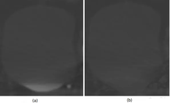
) , φ(o) is the neighborhood and h is a decay parameter. The underlying idea behind this filter is to replace a pixel belonging to a probable artifact by its nearest “foreground/background” model. Examples of the RoI pre-processing are depicted in Figure 3.

2.3. Multi-scale CT edge detector: the observations

The multiscale image analysis was herein implemented using the first partial derivatives at each scale obtained by convolving each RoIo(x, y) with a variable gaussian kernel. Thus,

the multi-scale edge estimation was obtained by a simple linear combination of the different gradient magnitudes at each scale, as follows:

S_oedge(x, y; σ) =X i RoIo(x, y) ∗ ∂Gσi ∂x∂y (5)

Figure 3. In (a) Bladder RoI preprocessing before. Lower bladder region had different appareance because filling bladder. In (b) is shown the processed RoI. The proposed filter reduce the appareance difference allowing capture robust observations

where Gσi is the 2D Gaussian function with standard deviation σi. In this context, the

Gaussian function is the unique kernel with an equivalent scale-space representation (linearity and shift-invariance in both frequency and space). A multiscale image decomposition allows to build a more stable set of observed edges [44] since true edges are coherently present at different scales. In this context, the detection of the boundaries is further pursued by applying a classical multiscale non-maximum suppression strategy, consisting in detecting the maximum gradient magnitude for each particular direction as cited in[44]. This multi-scale edge detection follows the universal principle of multi-scale invariance and allows a robust edge description which is usually preserved through multiple scales [45].

2.4. Computing the geometrical likelihood

Within a Bayesian framework, the devised likelihood function P( bSopcaj |S

edge

o ) was defined to

find the best geometrical matching between the sample shapes bSopcaj , obtained from the learned

model, and each multi scale edge descriptor S_oedge under a log-Euclidean metric [31]. For doing so, every shape, from the organ space, and the edges of each RoI, are characterized by the first seven Hu moments [8] as

P(SP CA oi |S edge oi ) = [min S_ojpca    X hu(i=1...7) ||mSoedge i − m S_ojpca i ||    (6) where mSoedge i = log |h Soedge i |, and m S_ojpca i = log |h S_ojpca

i | are the computed shape features for

the edges and the PCA learned shapes, respectively, and hSedge

i , h S_jpca

i are their Hu moments.

Under a log-Euclidean metric, null values are excluded, and the metrics allows to globally determine the most similar shape. This choice is also justified since the space of organs has a Lie group structure, that is to say, a similarity space in which continuity applies and algebraic operations are smooth mappings. This type of log-Euclidean metrics is invariant to orthogonal transformations, change of coordinates and scaling, and sets to an infinity distance those matrices with null or negative eigenvalues. The likelihood function reaches a maximal

probability when a learned shape closely match the observations after the multi-edge-scale descriptor.

2.5. Local Shape Deformation

In a final step, a 3D local deformation function was also introduced to eventually improve the local correspondence of the chosen organ, selected by the PCA model. Such deformation depends on two different measurements: (1) the radial distance of a particular shape point to the observed multi-edge-scale in the same slice and (2) the distance of the same particular organ point to the corresponding organ point in the upper and lower slices. These distances drive out the warping deformation of the organ either to the observed multi-edge-scale or to the upper and lower organ neighboring points. This deformation is controlled by a λ term, which represents a trade-off between the observed edge and the prior organ shape.

Soi(x, y) = λ bSopcai (x, y) + (1 − λ)(min_S o (k b

S_opca_{i − {So}edge_i , bS_opca_i±1}k))

This local deformation tends to preserve a coherence between the prior shape and the observed edges, a compact representation of the shape given by the λ term and the nearest edge criterion. In this work, the best performance was obtained from a training database with λ= 0.6

2.6. Experimental Setup

A quantitative comparison was performed between the manual organ delineations (prostate, bladder, rectum) and the computed segmentation, using two different measures: a dice score (DSC) and the Hausdorff distance. The DSC is an overlapping similarity measure, defined as DSC(A, B) = _|A|+|B|2|A∩B|, where _{| · | indicates the number of voxels of the considered} A (gold standard) and B volumes. On the other hand, the Hausdorff measure H(A, B) computes the maximum distance between two set of points as max(h(A, B), h(B, A)) and h(A, B) = maxa∈Aminb∈Bka − bk2₂. In this case, each set of points represents the organ

surface. This measure allows to indirectly assess the segmentation compactness.

As mentioned before, the dataset was randomly split into: training (30 patients) and test (86 patients). The training set was used to build the organ shape space and the best representation was selected within a leave-one-out cross validation scheme. The performance of the proposed method during the training step was compared with three multi-atlas vote methods_{‡, using a leave one out scheme. In a first multi-atlas method, the atlases were rigidly} registered to the test volume. The other two methods followed two steps: (1) the atlases were rigidly registered to the whole set of volumes, using a “block matching” strategy, and the transformed volumes were ranked according to the normalized cross-correlation (NCC) [43]. (2) The delineations associated to each volume were propagated to a new test organ volume by non-rigidly propagating the whole set of organs. This non-rigid registration was carried out by either a standard free-form deformation (FFD) [46] or by using the demons algorithm

[50]. Eventually, the majority vote decision rule was applied to obtain a single segmentation for each considered organ. A second evaluation of the presented method was carried out by segmenting the test data (86 patients) that were not included in the training phase, using the best prior model constructed during the training step.

3. Data

Data used in this paper include a total of 116 patients, who underwent Intensity Modulated Radiotherapy (IMRT) for localized prostate cancer between July 2006 and June 2007 in the same institution. The whole treatment (patient positioning, CT acquisition, and volume delineations) and dose constraints complied with GETUG 06 recommendations, as previously reported [14]. The size of the planning CT images in the axial plane was 512x512 pixels, with 1mm image resolution, and 2mm slice thickness. The used treatment planning system was Pinnacle V7.4 (Philips Medical System, Madison, WI). Each treatment plan used five field beams, in a step-and-shoot delivery configuration with gantry angles of 260◦, 324◦, 36◦, 100◦and 180◦. The delivery was guided by means of an IGRT protocol, with cone beam CT images or two orthogonal images (kV or MV imaging devices), using gold fiducial markers in 57% of patients. In this study, only the CT and the delineated prostate, bladder and rectum, were considered. For evaluation purposes, the dataset was split into two parts : training (30 patients) and test (86 patients) datasets.

4. Evaluation and Results

Figure 2 illustrates an example of segmentation obtained with the proposed approach (red), overlaid on an expert segmentation (in green). A major advantage of the proposed method is the adaptability of the prior shapes to the patient-specific organ, with local variations. As mentioned above, the approach performance was evaluated as follows:

4.1. Evaluation of training data

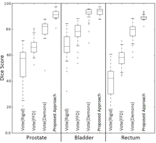
In a first experiment, by using the 30 patient randomly selected from the 116 available cases a DSC leave-one-out cross validation exploratory analysis was performed. Since DSC estimates the percentage of overlapping area between the evaluated segmentations, the obtained score is strongly dependent on the volume of the organs to be evaluated. Figure 3 shows the results obtained when comparing the presented approach with the three atlas based methods. The graph depicts the mean DSC and standard deviation for the four different automatic methods. The average score observed for the proposed method was of _{0.91 ± 0.033 for the prostate,} 0.94 ± 0.028 for the bladder, and 0.89 ± 0.022 for the Rectum. Overall, in terms of the DSC, the presented approach outperforms the atlas-based method (using the Demons) for the the prostate and rectum, by 9 %, and 9.2 % (p < 0.001), respectively, while for the bladder a slight gain of1.2 % was observed. Likewise, it should be noted that in all cases the standard deviation of the proposed approach is much smaller than the atlas based approaches.

Figure 4. Axial segmentation illustration of the pelvic structures ((a) rectum, (b) bladder and (c) prostate). The delineation obtained by the presented method (red) and the expert reference (green).

Figure 5. Dice scores comparison for vote vs the proposed approach

An additional comparison was performed by computing the Hausdorff Distance, which allows for the compactness of the segmentation to be compared since this measure penalizes the isolated voxels that are far from the ground truth. Table 1 summarizes the obtained performance for the three target organs, with smaller values for the proposed method in any case, indicating that the method coherently finds shapes compatible with the knowledge stored in the bank of shape organs. These results in addition illustrate that the presented approach systematically obtains shape segmentations with average distances of 5.98 for the prostate, 19.09 for the bladder and 7.52 for the rectum, while with the best atlas approach, the average distances were9.33 for the prostate, 79.42 for the bladder and 61.44 for the rectum. It should

Table 1. The Hausdorff distances obtained with the multi-atlas majority-vote method using rigid, FFD or a demons registration and with the proposed approach

Hausdorff Distance (mm) Segmentation methods Prostate Bladder Rectum

Vote(Rigid) 16.61±5.6 102.02±26 66.87±10.3

Vote(FFD) 14.27_±4.2 78.63_±20.1 65.22_±6.1

Vote(Demons) 9.33±3.2 79.42±18.2 61.44±5.8

proposed approach 5.98±2.2 19.09±3.1 7.52±2.3

be strengthen out that the Hausdorff distance evaluates not only the superposition of two shapes but also the quantity of scattered voxels that are outside of the segmented prostate: the larger the measure the higher the number of outlier voxels.

The results, obtained with this metric, point put the importance of using structural priors that define a particular topology. The bladder segmentation, calculated with the three atlas-based approaches and compared with the gold standard under the DSC metric, seemed to be appropriate, but when using the Hausdorff distance, larger differences appeared and produced a very large error of79.42 mm in the present study.

4.2. Evaluation of test data

Once a particular organ model was set, its generalization capacity was also evaluated. The best prior, determined by the PCA in the previous experiment with 30 patients, was used in a second test group with 86 patients, a larger data set with different shape organs, presence of artifacts or contrast changes in CT. Quantitative results, with the previously introduced metrics, are reported in table 2. In general terms, the obtained results show a segmentation, with an averaged DSC of0.86 and an averaged Hausdorff Distance of 16.19. The befitting obtained segmentations are consistent with what was observed in the training data, i.e. with a best score for the bladder. This fact can also be attributed to the overlapping measure since results depend on the organ volume. Although the obtained score errors are slightly larger for the three organ segmentations, the proposed approach properly captures the shape variability. The Hausdorff distance, on the other hand, shows that the proposed approach produces more stable segmentations, meaning that voxels belong mostly to a single shape since the measurement penalizes the isolated or outlier voxels. Unlike the atlas based approaches, this method reaches a tolerable margins of error, an important element when planning the radiation therapy. Finally, in both quantitative metrics, the obtained standard deviation was lower, evidencing coherency in the obtained segmentations.

5. Discussion

An automatic method for segmentation of pelvic organs in CT images was presented. Under a Bayesian framework, a geometrical likelihood function mapped a set of global observations, built from a structural multi-scale analysis [44], to a prior shape space that stored the shape

Table 2. The Dise score and the Hausdorff distances obtained the proposed approach in using the test data

Macro name Prostate Bladder Rectum

Hausdorff Distance (mm) 9.98±3.4 25.07±4.6 13.52± 5.1 Dice score (DSC) 0.87± 0.071 0.89± 0.083 0.82± 0.062

organ knowledge. This prior captured the principal shape variation modes, constituting an organ space with samples that represent the 96 % of the shape variability [40, 16]. Observations were automatically captured from RoIs around each specific organ, namely, the prostate, the bladder and the rectum. Each of these RoIs is pre-processed by an adapted non-local filter which regularizes the region by considering only two principal pixel distributions: the organ and the background. This filter allows for artifact reduction coming from gas in the rectum, several filling bladder states or bone parts randomly captured within the RoI. Afterward, a set of structural observations, the Hu moments, are calculated from a multi-edge-scale feature. The obtained Hu-based descriptor is a global shape representation that is used by a geometrical likelihood function to find the most likely organ shape given the set of observations. The likelihood function rules out the null Hu moments and redistributes the organ space using a log-Euclidean metrics and thereby it matches the most similar.

In general, state-of-the-art methods attempt to obtain more accurate segmentations by integrating a prior to the CT image information, for instance the CT or MRI manual expert delineations or CT salient morphological points. The Bayesian approach herein presented may be included in statistical shape models family since the organ shape prior is mapped to the CT through a geometrical likelihood. Several statistical models, for segmenting CT registered structures, have been proposed. Among them, a semi-automatic Bayesian method that matches a set of organ templates and finds the most probable template transformation using an iterative increasing and bending algorithm may be found in [29]. Each of these templates is characterized by a medial axis relationship at different resolution scales. However, the media axis result in many cases very simple shape representation that can lead to wrong segmentations since the growing iterative algorithm can easily overflow the pelvic organ boundary. Likewise, segmentation of the prostate and rectum has been also approximated using a histogram learning representation under a Bayesian framework [25], achieving an average volume overlapping of0.89 and 0.71, for the prostate and rectum, respectively. These low figures can be attributed to the histogram representation since (1) it is not robust to contamination with any complex noise, (2) some bladder states and bone structures show practically the same gray level, (3) there exists a high inter patient variability regarding the bladder state and (4) it completely misses the spatial relationships.

Essentially, the proposed approach combines both a multi-scale (global) and derivative estimations (local) to obtain the real organ edges. Since organ boundaries in the CT images are usually very blurred and even experts can miss actual boundaries, the proposed approach sets a proper edge estimation using a likelihood function that uses global metrics (The Hu moment characterization) of the searched shape and then corrects for the possible edge mismatches.

Another advantage of the proposed approach is the use of prior shapes by the likelihood function so that voxels belonging to any organ shape are always connected. This investigation has extended the usual prostate segmentation to the whole set of organs at risk, with very little change in the required parameters. The method has demonstrated to be robust to many types of noise and adaptable to different organs, with comparable accuracy values when segmenting the prostate, the bladder or the rectum. The approach was compared to 3 different atlas based methods which also included geometrical prior information, using the DSC and Hausdorff distance calculated between the automatic organ segmentation and a manual delineation carried out by a radiologist expert. Patients were grouped in training and test groups, and in both scenarios the proposed approach outperformed the other methods.

Finally, several pre-processing strategies have been proposed to overcome the natural high intra and inter patient organ appareance variability, for instance, Davis et al [28] cope with the bowel gas problem by defining a binary mask containing the regions with gas. Then, they apply a “deflation” transformation, based on the flow computed or induced by the binary image mask, and doing that this region tend to converge to the center of these regions. These approximation allows to reduce the bowel gas effect but without taking into account that very often this phenomenon appears as scattered in small regions. In the proposed approach, a new non-local filter which replaces the RoI artifacts was introduced. Taking advantage of the redundancy and assuming that a segmented RoI is composed of two tissues: organ and background. This facilitates the organ segmentation, above all because some organs like the bladder or rectum are composed of different objects that result in different distributions, this filter allows to homogenize the organ texture and to isolate the concept. After this filter, an organ and background pixel distribution are may be facilitated and used thereafter. Last but not least, the obtained results are highly encouraging and demonstrate the method usefulness in clinical scenarios as a support of the final delineation that dramatically decreases the expert burden in the daily radiotherapy planning.

6. Conclusions and Perspectives

We presented in this work is a new methodology to segment pelvic structures in CT scans. The Bayesian method combines a deformable prostate model, learned from examples, and a geometrical likelihood strategy that maps actual observation into the space of model organs and selects the best shape to superimpose it in the original CT image. The presented results offer that this segmentation technique may be suitable to use as a oncologist’s support. This approach may be easily extended to other structures in CT images. Future works includes a more robust CT characterization by the association of edge observation and pixel distributions in order to find more likely shapes in the organ space and also develop a more reliable local shape adjustment.

Acknowledgements

This work is partially supported by Rennes Metropole through a mobility scholarship and the project ANR TIGRE.

References

[1] D’Amico, et al: Biochemical outcome after radical prostatectomy, external beam radiation therapy, or interstitial radiation therapy for clinically localized prostate cancer. AMA 280 (1998)

[2] Micheli-Tzanakou, Evangelia and Rohlfing, Torsten and Brandt, Robert and Menzel, Randolf and Russakoff, Daniel and Maurer, Calvin &lt;i&gt;Quo Vadis&lt;/i&gt; , Atlas-Based Segmentation Handbook of Biomedical Image Analysis. Springer US. 435–486 (2005)

[3] Hodge, A.C., Fenster, A., Downey, D.B., Ladak Prostate boundary segmentation from ultrasound images using 2D active shape models: Optimisation and extension to 3D. Comput. Methods Programs Biomed. 84(2-3) 99–113 (2006)

[4] Oscar Acosta and Gael Drean and Juan D Ospina and Antoine Simon and Pascal Haigron and Caroline Lafond and Renaud de Crevoisier Voxel-based population analysis for correlating local dose and rectal toxicity in prostate cancer radiotherapy Physics in Medicine and Biology. 58(8) 2581 (2013)

[5] V. Beckendorf and J. M. Bachaud and P. Bey and S. Bourdin and C. Carrie and O. Chapet and D. Cowen and S. Guérif and H. M. Hay and J. L. Lagrange and P. Maingon and E. Le Prisé and P. Pommier and J. M. Simon Target-volume and critical-organ delineation for conformal radiotherapy of prostate cancer: experience of French dose-escalation trials Cancer Radiother. 6(1) 78–92 (2002)

[6] Bagshaw MA, Cox RS, Ramback JE. Radiation therapy for localized prostate cancer. Justification by long-term follow-up. Urol Clin North Am.17(4)787-802.(1990)

[7] Perez CA, Michalski J, Mansur D. Clinical assessment of outcome of prostate cancer (TCP, NTCP). Rays.30(2):109-20. 2005

[8] D. Zhang: Review of shape representation and description techniques. Pattern Recognition, 37(1):1-19, 2004.

[9] Heemsbergen, W.D., et al: Urinary obstruction in prostate cancer patients from the dutch trial (68 gy vs. 78 gy): Relationships with local dose, acute effects, and baseline characteristics. Int J Radiat Oncol Biol Phys (2010)

[10] Acosta, O.,et al: Atlas based segmentation and mapping of organs at risk from planning CT for the development of voxel-wise predictive models of toxicity in prostate radiotherapy. In:Prostate Cancer Imaging. International Workshop in MICCAI 2010. LNCS 6367. 42–51. (2010)

[11] B. Al-Qaisieh et al. Impact of prostate volume evaluation by different observers on CT-based post-implant dosimetry Radiother Oncol. 62 (3) 267–273. (2002)

[12] Bayley A, Rosewall T, Craig T, Bristow R, Chung P, Gospodarowicz M, Ménard C, Milosevic M, Warde P, Catton C. Clinical application of high-dose, image-guided intensity-modulated radiotherapy in high-risk prostate cancer. Int J Radiat Oncol Biol Phys. 77(2) 477–83. (2010)

[13] Jeff Bilmes A Gentle Tutorial of the EM Algorithm and its Application to Parameter Estimation for Gaussian Mixture and Hidden Markov Models. Tech. Rep., 1998

[14] Véronique Beckendorf and Stéphane Guerif and Elisabeth Le Prisé and Jean-Marc Cosset and Agnes Bougnoux and Bruno Chauvet and Naji Salem and Olivier Chapet and Sylvain Bourdain and Jean-Marc Bachaud and Philippe Maingon and Jean-Michel Hannoun-Levi and Luc Malissard and Jean-Jean-Marc Simon and Pascal Pommier and Men Hay and Bernard Dubray and Jean-Léon Lagrange and Elisabeth Luporsi and Pierre Bey 70 Gy versus 80 Gy in localized prostate cancer: 5-year results of GETUG 06 randomized trial Int J Radiat Oncol Biol Phys. 80(4) 1056–1063. (2011)

[15] Costa, María Jimena and Delingette, Hervé and Novellas, Sébastien and Ayache, Nicholas: Automatic Segmentation of Bladder and Prostate Using Coupled 3D Deformable Models. MICCAI 2007. LNCS. 252–260. (2007)

[16] T. Cootes and C. Taylor. Statistical models of appearance for medical image analysis and computer vision In Proc. SPIE Medical Imaging. (2001) 236–248

[17] Söhn M,et al: Dosimetric treatment course simulation based on a statistical model of deformable organ motion. Phys. Med. Biol. 57 (2012) 3693

[18] Collier, D., Burnett, S., Amin, M., Bilton, S.,et al: Assessment of consistency in contouring of normal-tissue anatomic structures. Journal of Applied Clinical Medical Physics. 4 (2003)

[19] Fiorino, C. and Reni, M. and Bolognesi, A. and Cattaneo, G.M. and Calandrino, R. Intra- and inter-observer variability in contouring prostate and seminal vesicles: implications for conformal treatment planning. Radiother Oncol. 47(3)(1998) 285–292

[20] K.M Langen and D.T.L Jones: Organ motion and its management. International Journal of Radiation Oncology-Biology-Physics. 50 (2001) 265–278

[21] G Bueno, A Martínez-Albalá, Adán Fuzzy-snake segmentation of anatomical structures applied to ct images ICIAR (2). (2004) 33–42

[22] Gual-Arnau X, Ibánez Gual, Lliso F, Roldán S Organ contouring for prostate cancer: Interobserver and internal organ motion variability Computerized Medical Imaging and Graphics. 29 (2005) 639–647 [23] Guckenberger M, Flentje M. Intensity-modulated radiotherapy (IMRT) of localized prostate cancer: a

review and future perspectives. Strahlenther Onkol. 183(2) 57 –62.(2007)

[24] Siqi Chen and D. Michael Lovelock and Richard J. Radke: Segmenting the prostate and rectum in CT imagery using anatomical constraints. Medical Image Analysis. 15 (2011) 1–11

[25] Siqi Chen and D. Michael Lovelock and Richard J. Radke: Segmenting the prostate and rectum in CT imagery using anatomical constraints. Medical Image Analysis. 15 (2011) 1–11

[26] Rohlfing, T and Maurer, CR Multi-classifier framework for atlas-based image segmentation Pattern Recognition Letters. 26 (13) (2005) 2070 –2079

[27] Li W, Liao S, Feng Q, Chen W, Shen D. Learning image context for segmentation of the prostate in CT-guided radiotherapy. Physics in Medicine and Biology. 57 (2012) 1283.

[28] Davis BC, Foskey M, Rosenman J, Goyal L, Chang S, Joshi S. Automatic segmentation of intra-treatment CT images for adaptive radiation therapy of the prostate. Med Image Comput Comput Assist Interv. 8 (2005) 442–50.

[29] Sarang Joshi and Stephen Pizer and P. Thomas Fletcher and Paul Yushkevich and Andrew Thall and J. S. Marron. Multiscale deformable model segmentation and statistical shape analysis using medial descriptions. Transactions on medical imaging. 21 (5) 2012 538 –550

[30] Martínez F., Acosta O., Dréan G., Antoine S., Pascal H., Crevoisier R.. Romero E. Segmentation of pelvic structures from planning CT based on a statistical shape model with a multiscale edge detector and geometrical likelihood measures. Image-Guidance and Multimodal Dose Planning in Radiation Therapy. International Workshop in MICCAI 2012.

[31] Fast and Simple Calculus on Tensors in the Log-Euclidean Framework Arsigny, Vincent and Fillard, Pierre and Pennec, Xavier and Ayache, Nicholas Medical Image Computing and Computer-Assisted Intervention MICCAI (2005) 115–122

[32] Rousson, Mikael and Khamene, Ali and Diallo, Mamadou and Celi, Juan and Sauer, Frank: Constrained Surface Evolutions for Prostate and Bladder Segmentation in CT Images. Computer Vision for Biomedical Image Applications. Springer Berlin / Heidelberg (2005)

[33] Pekar, V., McNutt, T.R., Kaus, M.R., Automated model-based organ delineation for radiotherapy planning in prostatic regions. Int. J. Radiat. Oncol. Biol. Phys. 3 (2004) 973–980

[34] Feng, Qianjin and Foskey, M. and Tang, Songyuan and Chen, Wufan and Shen, Dinggang: Segmenting CT prostate images using population and patient-specific statistics for radiotherapy deformable models. IEEE ISBI. (2009) 282–285

[35] D. Bystrov, et al: Simultaneous fully automatic segmentation of male pelvic risk structures. In: Estro. European society for Radioherapy and oncology. (2012)

[36] Rohlfing, et al: Multi-classifier framework for atlas-based image segmentation. Computer Vision and Pattern Recognition, IEEE Computer Society Conference on 1 (2004) 255–260

[38] Isgum, I., et al: Multi-atlas-based segmentation with local decision fusion - application to cardiac and aortic segmentation in CT scans. IEEE Transactions on Medical Imaging 28 (2009) 1000–1010 [39] Acosta, O., et al: Evaluation of multi-atlas-based segmentation of ct scans in prostate cancer radiotherapy.

IEEE ISBI. (2011) 1966 –1969

[40] Heimann, T., Meinzer, H.P.: Statistical shape models for 3d medical image segmentation: A review. Medical Image Analysis 13 (2009) 543 – 563

[41] Sohn, M., et al: Modelling individual geometric variation based on dominant eigenmodes of organ deformation: implementation and evaluation. Physics in Medicine and Biology 50 (2005) 5893 [42] Lorenz, C.,et al: Generation of Point-Based 3D Statistical Shape Models for Anatomical Objects. CVIU

77 (2000) 175–191

[43] Ourselin, S., et al: Reconstructing a 3D structure from serial histological sections. Image and Vision Computing 19 (2001) 25 – 31

[44] Lindeberg, T.: Feature detection with automatic scale selection. Int. J. Comput. Vision 30 (1998) 79–116 [45] Ter Haar Romeny,et al: Scale space: Its natural operators and differential invariants. In Colchester.:

Information Processing in Medical Imaging. Springer Berlin / Heidelberg (1991) 239–255

[46] Rueckert, D., et al: Nonrigid registration using free-form deformations: Application to breast mr images. IEEE Transactions on Medical Imaging 18 (1999) 712–721

[47] Minjie Wu and Caterina Rosano and Pilar Lopez-Garcia and Cameron S Carter and Howard J Aizenstein Optimum template selection for atlas-based segmentation. Neuroimage. 34(4) (2007)1612–1618 [48] Liao, Shu and Gao, Yaozong and Shen, Dinggang. Sparse Patch Based Prostate Segmentation in CT

Images Medical Image Computing and Computer-Assisted Intervention MICCAI (2012). (3) 385-392 [49] Yaozong Gao, Shu Liao, Dinggang Shen Prostate segmentation by sparse representation based

classification Medical Image Computing and Computer-Assisted Intervention MICCAI (2012). (3) 451-458

[50] Thirion, J.P.: Image matching as a diffusion process: an analogy with maxwell’s demons. Medical Image Analysis 2 (1998) 243 – 260