Formation and coarsening of roll-waves in shear shallow water flows down an inclined rectangular channel

HAL Id: hal-01527469

https://hal.archives-ouvertes.fr/hal-01527469

Submitted on 24 May 2017

HAL is a multi-disciplinary open access

archive for the deposit and dissemination of

sci-entific research documents, whether they are

pub-lished or not. The documents may come from

teaching and research institutions in France or

abroad, or from public or private research centers.

L’archive ouverte pluridisciplinaire HAL, est

destinée au dépôt et à la diffusion de documents

scientifiques de niveau recherche, publiés ou non,

émanant des établissements d’enseignement et de

recherche français ou étrangers, des laboratoires

publics ou privés.

Formation and coarsening of roll-waves in shear shallow

water flows down an inclined rectangular channel

Kseniya Ivanova, Sergey Gavrilyuk, Boniface Nkonga, Gaël Loïc Richard

To cite this version:

Kseniya Ivanova, Sergey Gavrilyuk, Boniface Nkonga, Gaël Loïc Richard. Formation and coarsening of

roll-waves in shear shallow water flows down an inclined rectangular channel. Computers and Fluids,

Elsevier, 2017, 159, pp.189-203. �hal-01527469�

Formation and coarsening of roll-waves in shear

shallow water flows down an inclined rectangular

channel

K.A. Ivanova

, S.L. Gavrilyuk

, B. Nkonga

, G.L. Richard

Abstract

The formation of a periodic roll-wave train in a long channel is studied for two sets of experimental parameters (noted as Case 1 and Case 2) corresponding to Brock’s experiments [3], [4]. In both cases, a formed free surface profile was found in a very good agreement with the experimental results. Mathematical properties of the model were also tested in the case where the perturbation frequency was lower than the experimental one, so longer waves were generated at the channel inlet. It was observed that the amplitude and the enstrophy of the corresponding roll-waves train are strongly modulated. In the case where the waves of two different lengths were generated at the channel inlet, the coarsening was observed. The coarsening phenomenon is always accompanied by a strong modulation. A comparison with the Saint-Vennat equations is also done.

The formation of a single wave composing a roll-wave train was also studied in a domain with periodic boundary conditions (called “periodic box”) for the same sets of experimental parameters. The free surface profile was found also in a very good agreement with the experi-mental results. This allows us to justify the use of the “periodic box” as a simple mathematical tool for a qualitative study of roll-waves stability. In particular, we studied the stability of a single steady wave by increasing its length. It was shown that the wave becomes morphologi-cally unstable after some critical wave length : it transforms into a system containing several waves. It is also proved that a single steady wave corresponding to Case 1 is stable under multi-dimensional perturbations in the framework of a model which is a simplification of a general multi-D model of shear shallow water flows.

Keywords : shear shallow water flows, roll-waves, coarsening, hyperbolic equations, Godunov

method

1

Introduction

Uniform fluid flows with a free surface down an inclined plane are unstable if the inclination angle is larger than some critical value. The flow then transforms into a system of breaking waves usually called “roll-waves”. Brock [4] measured the permanent wave profiles obtained by introducing periodic disturbances at the channel inlet and in different conditions (different slopes and wall roughness). He also studied natural roll-waves propagating in nonperiodic manner. He noticed that the roll wave profiles always contained the following three essential parts: first, a steeply sloping wave front, second, a continuous zone where the depth increases progressively, and third,

∗_{Aix-Marseille Universit´e, C.N.R.S. U.M.R. 7343, IUSTI, 5 rue E. Fermi, 13453 Marseille Cedex 13 France,}

kseniya.ivanova@univ-amu.fr

†_{Corresponding author, Aix-Marseille Universit´e, C.N.R.S. U.M.R. 7343, IUSTI, 5 rue E. Fermi, 13453 Marseille}

Cedex 13 France, sergey.gavrilyuk@univ-amu.fr and Novosibirsk State University, 2 Pirogova, 630090 Novosibirsk, Russia

‡_{Universit´e de Nice Sophia-Antipolis, C.N.R.S. U.M.R. 7351, Laboratoire J.A.Dieudonn´e, Parc Valrose, 06108}

NICE Cedex 2 France, Boniface.Nkonga@unice.fr

§_{Institut de Math´ematiques de Toulouse; U.M.R. 5219, Universit´e de Toulouse, C.N.R.S. , UPS IMT, F-31062}

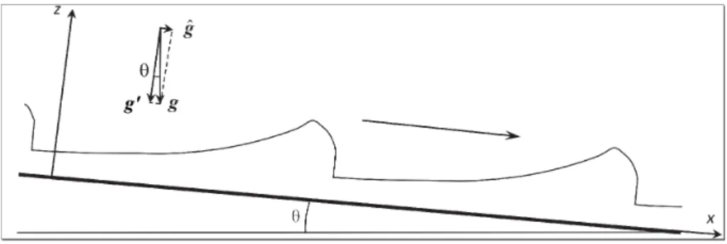
Figure 1: Sketch of a typical profile of roll waves down an inclined plane of angle θ in Brock’s experiments (1967).

a slowly decreasing zone until reaching a new hydraulic jump (see Figure 1). The second part of the stationary wave profile corresponds to a flow region with a strong vorticity riding the wave front (called also “roller”). This part of the profile is absent when the classical Saint-Venant (SV) equations are used (Dressler, 1949) [5]. Recently, a new model of shear shallow water flows was developed in Richard & Gavrilyuk (RG) (2012, 2013)[12], [13], describing, in particular, the roller formation. With such a model, it was shown that the permanent roll-waves profiles correspond to experimental ones with a good accuracy. A common characteristics of solutions obtained in Dressler (1949)[5] and Richard & Gavrilyuk (2012) [12] is that they form a one-parameter family of solutions parametrized by the wave length. Roughly speaking, for a given flow discharge, roll-waves of different lengths (and, consequently, different amplitudes) may exist. However, it is quite obvious that very long waves (large amplitude waves) can not exist. So, a natural question arises whether the permanent roll-waves of all lengths are stable in this model. The answer to this question is not at all trivial, and several important studies were performed on this subject. The modulational stability of Dressler waves for SV model was studied, in particular, in Liapidevskii & Teshukov (2000)[9] and Liapidevskii & Boudlal (2002) [2]. They have shown that for any Froude

number larger than two, there exists an interval (Lmin, Lmax) such that the waves of the length

belonging to this interval are stable. The waves of smaller or greater lengths are unstable in the sense that the corresponding modulation equations loss their hyperbolicity. Barker et al.[1]) studied the spectral stability of roll-waves for viscous SV equations. Stability diagrams at the plane “Froude number-wave length”, in particular, were constructed. The spectral instability of small length non-viscous roll-waves for SV equations was also proved in [17]. The new system derived in Richard & Gavrilyuk (RG) (2012, 2013) contains one equation more, so the stability analysis is more difficult. This is why we propose here a numerical approach to the roll-wave stability study. We study a roll-waves formation through a non-stationary process. If the waves are formed, they are stable, if not, they are not stable. Also, different scenarios of a roll-wave train formation appearing in numerical study could give an important information for practical applications. In particular, the wave “coarsening” produced by irreversible coalescence of non-stationary roll-waves will be studied. The numerical study of roll-waves formation for the SV model was performed earlier in [18].

This paper is divided into five sections. The governing equations for the shear shallow-water theory are presented in Section 2. The corresponding finite-volume Godunov type discretization methods are described in Section 3. The numerical results concerning the roll-waves formation, the comparison with Brock’s experiments and with numerical solutions of SV equations are presented in Section 4. The study of a 2D simplified model of shear shallow water flows is presented in the Section 5. The Appendix gives the description of a higher-order extension of Godunov’s method.

2

Governing equations

Studied one-dimensional governing equations describing shear shallow water flows on an inclined plane, represent a system of non-linear conservation laws of mass, momentum and energy with source terms describing the balance between gravity and friction. They are (Richard & Gavrilyuk, 2012, 2013)[12], [13]: ∂h ∂t + ∂hU ∂x = 0, (1) ∂hU ∂t + ∂ ∂x ( hU2+ p)= ˆgh− CU|U|, (2) ∂ ∂t(hE) + ∂ ∂x(hU E + pU ) = (ˆgh− CeU|U|) U. (3)

Here h is the fluid depth, U is the average velocity, g′= g cos θ, ˆg = g sin θ, θ is the inclination

angle, C is the Ch´ezy coefficient (friction coefficient) corresponding to the dissipation in the

momentum equation, Φ is the enstrophy (squared vorticity) of large eddies formed in the roller,

Ce= C + CrΦ/ (φ + Φ). The coefficient Cris the dissipation coefficient in the jump roller, and φ

is the enstrophy of small eddies developed near the bottom. It is supposed to be constant. The total specific energy E, the “internal energy” e, the “pressure” p are defined as

E = 1 2U 2_{+ e, e =} 1 2 ( g′h + (φ + Φ)h2), (4) p = g ′_h2 2 + (φ + Φ)h 3_{. (5)}

The second term in the expression for the “internal energy” e is the sum of the “turbulent” kinetic

energy in the roller ( 1

2Φh

2_{), and the “turbulent” kinetic energy in the boundary layer (}1

2φh 2_). The system (1), (2), (3) admits the following equation for the enstrophy Φ:

DΦ

Dt =

2

h3(C− Ce)|U|

3_{< 0. (6)}

System (1), (2) and (3) is a time-dependent system of non-linear hyperbolic partial differential

equations with characteristic speeds given by: U and U± as, where asis the speed of the surface

waves. It plays the role of the “sound speed” in this model and defined as follows as=

√

g′h + 3(φ + Φ)h2_{. (7)}

This system is derived in the framework of the shallow water approximation theory, when the ratio of water depth to the wave length is small and by averaging over the fluid depth. Also an additional hypothesis about the horizontal velocity shear smallness was supposed. The equation

(6) means that the enstrophy is decreasing along the trajectories, if C < Ce. Since the equations

are reminiscent of the Euler equations of compressible fluids, the conservation laws imply standard Rankine–Hugoniot relations. At the shock front, the enstrophy is increasing analogously to the entropy increase for the Euler equations of compressible flows. The enstrophy production at the shocks corresponds physically to the “roller” formation. Then the enstrophy dissipates over the

length of the roller according to (6). When one takes φ = 0, Φ = 0, and C = Ce, the system is

reduced to the classical Saint-Venant equations.

The system (1) - (3) can be rewritten in conservative form :

Ut+ F(U)x= S(U), (8)

where the vector of the “conserved” variables U, the vector of fluxes F(U) and the source term vector S(U) are:

U =   hUh hE   , F(U) =   hUhU2_{+ p} hU E + pU   , S(U) =   ghˆ − C|U|U0 (ˆgh− Ce|U|U) U   .

We will study the roll-waves formation by two methods. The first one is a direct numerical study of the roll-waves formation in a long channel from a uniform unstable flow. The flow is perturbed by a wave maker at the inlet of the channel (situated for definiteness at x = 0) with a given constant flow discharge. The second method consists in the roll-waves formation in a

“periodic box” : the outcoming variables at x = Lb (subscript “b” means “box”) are the same

as the entering variables at x = 0. The initial velocity is also uniform, but the fluid depth is perturbed in such a way, that the averaged layer depth is equal to the unperturbed one. In this case we conserve the average depth, but not the average discharge.

The relation between these two approaches will be established later. The “periodic box”

method is more comfortable from the numerical point of view, because it allows us to study the large time flow behaviour, but the long channel study is physically more understandable.

2.1

Initial and boundary conditions for a long channel

We have to impose for (8) initial conditions for x belonging to the interval [0, L] (L is the length of the open channel), and the boundary conditions at x = 0 and x = L. The number of boundary conditions corresponds to the number of characteristics entering the flow domain. The initial conditions are :

h(x, t = 0) = h0= const, Φ(x, t = 0) = Φ0= 0, U (x, t = 0) = U0= √

gh0sin θ/C. (9)

This is an exact solution of our system. It is linearly stable, if the generalized Froude number F rg0=

U0 as0

(as0is the “sound velocity” at equilibrium) is smaller then 2, and linearly unstable in the opposite

case [12], [11]. Here we consider the unstable case to study the roll-waves formation. Since the flow is supercritical (the generalized Froude number is greater than one), three characteristics enter the domain at x = 0. So, we need three boundary conditions at x = 0:

h(x = 0, t) = h0(1 + a sin(ωt)), Φ(x = 0, t) = 0, U (x = 0, t) = q

h(x = 0, t). (10)

Here q = h0U0 is the flow discharge, a is a constant perturbation amplitude, ω is a constant

frequency. Since the flow is supercritical, we do not need to impose the boundary conditions for x = L (there is no characteristics entering the flow domain). The boundary condition for h allows us to model qualitatively a wave maker movement that was used by Brock at the channel inlet to accelerate the formation of roll-waves.

2.2

Initial and boundary conditions for a periodic box

We take periodic boundary conditions for the periodic box of length Lb :

U(0, t) = U(Lb, t), t≥ 0.

Consider the stationary unstable solution (h0, U0, Φ0= 0) where the equilibrium velocity U0 is

given by (9). Suppose that the generalized Froude number is greater than two. Assuming sinusoidal initial perturbation of amplitude a of the free surface :

h(x, t)|_t=0= h0 ( 1 + a sin ( 2πx Lb )) , (11)

and taking other variables constant

U|_t=0= U0, Φ|_t=0= 0, we allow the flow evolve in time.

3

Numerical scheme

We use here conservative, finite volume Godunov type scheme on a fixed grid. It requires the solution of the Riemann problem at every cell boundary at each time step [7], [8], [16], [14]. The MUSCL-Hancock extension of the Godunov method is used with the MinMod limiter for the depth, the velocity and the “pressure”.

3.1

Hyperbolic step

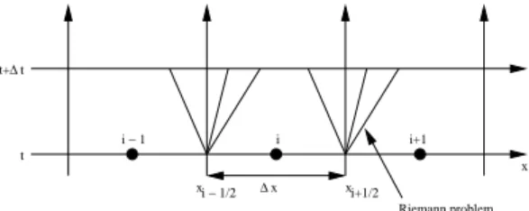
Let us consider a fixed grid of size ∆x = xi+1/2 − xi−1/2, the time increment is defined as

∆t = tn+1− tn that must respect the Courant-Friederichs-Lewy’s (CFL) condition (see Figure

2). The value of the CFL number is taken to be 0.8. The number of cells is always given for a converged solution. In particular, for such a solution every single roll-wave is represented at least

by 100 points. The discrete values of the vector-function U(x, t) at (xi, tn) will be denoted by

Un_i ≡ U(xi, tn).

The first step (hyperbolic one) consists in computing the source term-free system:

xi − 1/2 t t+∆t x ∆x _xi+1/2 i+1 i i − 1 Riemann problem

Figure 2: The fixed grid and Riemann problem.

Ut+ Fx= 0, (12)

with the initial condition for the complete problem U(x, tn_{) = U}n_{. Integrating in space and time}

[xi−1/2, xi+1/2]× [tn, tn+1] the conservation laws (12), one obtains a conservative finite volume

Godunov scheme on a fixed grid :

¯ Un+1_i = Un_i − ∆t ∆x ( F∗,n_i+1/2− F∗,n_i−1/2 ) , (13)

where F∗,n_i+1/2 and F∗,n_i−1/2 are the numerical fluxes. They are constant across interfaces between

cells during the time step. For computing the fluxes F∗,n_i+1/2 and F∗,n_i−1/2, we solve the Riemann

problems between cells i, i + 1 and i− 1, i, respectively (see Figure 2). The HLLC Riemann solver

is used for this (see Toro for details [16]). The second order extension is presented in Appendix.

3.2

Integrating the source terms

The second step is to integrate the ordinary differential equations dU

dt = S(U), (14)

with the initial condition U|t=0 = ¯Un+1 given by (13). The 4th order Runge-Kutta method is

TEST h0[m] θ [rad] Cr C φ [s−2] λ [m] ω [rad/s] T [s] F rg0 a

CASE 1 0.00798 0.05011 0.00035 0.0036 22.76 ≈ 1.3 6.73 0.933 3.63 0.05

CASE 2 0.00533 0.119528 0.002 0.0038 153.501 ≈ 1.8 6.19012 1.015 5.03 0.05

Table 1: Hydraulic parameters for two numerical tests corresponding to Brock’s measurements

[4] are given. The flow discharge q0 = h0U0 can be calculated by using (9) and the value of h0.

The amplitude value a is not given in [4]. The amplitude increase accelerates the formation of a

roll-wave train but does not influence its final form. The values Cr and C correspond to those

used in [12].

4

Numerical simulation of roll waves

Two sets of parameters are taken for the numerical study of the roll-waves formation in a long channel (see Table 1). In Case 2 the inclination angle is greater than that in Case 1. Consequently, the generalized Froude number and the wavelength are greater also in Case 2. The friction

coef-ficient C in both cases is approximately the same. In Table 1, Cr is the dissipation coefficient in

the jump roller, λ is the wave length, ω is the wave frequency, T is the period of perturbation, h0

is the initial depth, a is the perturbation amplitude. They will be used for the flow modelling in both a long channel and a periodic box. The length of the channel varied between L = 40 [m] and L = 600 [m]. For the periodic box we will use Lb of 1.3 m or 1.8 m, corresponding to Cases 1 and

2. We will also perform computations for a periodic box having a length multiple of Lb, with the

perturbation of the same type:

h(x, t = 0) = h0(1 + a sin(2πx/(nLb))), n = 2, 3, ... (15)

4.1

Long channel

In this section we will focus on the evolution of a roll-wave train moving down in a rectangular inclined open channel of a constant slope. For a prescribed average discharge, the Dressler theory gives a one-parameter family of solutions, parametrised by a wavelength ranging from zero to infinity. It was shown analytically for the SV equations [9], [2], [1] that not all waves are stable. We will obtain the analogous effect for the new (1)-(3) model. We perturb a uniform flow at the channel inlet (the perturbation amplitude is 5% of the uniform depth). First, we take the generalized Froude number smaller then two. As it was expected from the theory [12], [11], the perturbations move downstream the channel with decreasing amplitude until they completely disappear. Hence, a roll-waves train is not formed because the uniform flow is stable (see Figure 3). When we take the generalized Froude number larger than 2, the perturbations are amplified with time and are transformed rapidly to a roll-wave train. All waves have the same amplitude and propagation speed (Figures 4, 5). Each wave profile includes shock and a strongly sheared region after the shock (roller), where the depth continues to increase. The roller enstrophy increases through the shocks and then rapidly decreases over the roller length (Figures 4, 5).

The roll-waves are completely formed at a distance of about 15− 20 m from the channel inlet

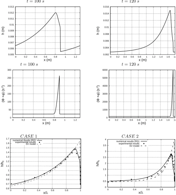
(in both cases). The length of a single roll wave is about 1.3 m (Case 1 ) and 1.8 m ( Case 2). In Figure 6 we compare a single roll-wave obtained for the model (1)–(3) with Brock’s measure-ments and the numerical solution of the SV equations. The profile of a single wave corresponds to that found in [11], [12]: a rapidly varying part (a jump), a gradual monotonic increase of the wave profile, and a decreasing part. A good agreement between stationary solution of the new model and the experiments is observed. We note that the amplitude of the jump is always smaller than the double of the depth before the jump. This is in accordance with the limit depth ratio com-ing from the Rankine-Hugoniot relations (see [11], [12]). One can observe an essential difference between the SV solutions and experimental observations.

It is interesting to understand what happens if the perturbation frequency is much lower than the experimentally chosen values. We have taken ω = 2.0 [rad/s]. Since single waves forming

0.0079 0.00792 0.00794 0.00796 0.00798 0.008 0.00802 0.00804 0.00806 0.00808 0 5 10 15 20 25 30 35 40 h (m) x (m) t = 100 s, F rg0< 2

Figure 3: A computed solution in the long channel of 40 m for the case of F rg0 = 1.15 is

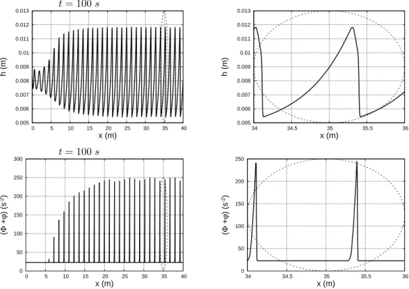
shown at time instant 100 s. The number of cells N = 8000. The roll waves are not formed as it is expected from the theory. The perturbation moves downstream the channel with rapidly decreasing amplitude. 0.005 0.006 0.007 0.008 0.009 0.01 0.011 0.012 0.013 0 5 10 15 20 25 30 35 40 h (m) x (m) 0.005 0.006 0.007 0.008 0.009 0.01 0.011 0.012 0.013 34 34.5 35 35.5 36 h (m) x (m) 0 50 100 150 200 250 300 0 5 10 15 20 25 30 35 40 ( Φ + ϕ ) (s -2) x (m) 0 50 100 150 200 250 34 34.5 35 35.5 36 ( Φ + ϕ ) (s -2) x (m) t = 100 s t = 100 s

Figure 4: Case 1. The roll-waves formation (at the left) and a magnified view (at the right) are shown both for the wave profile and the enstrophy.

such a roll-wave train have larger lengths, we took a longer channel, of 600 m long, to see better the structure of the final roll-wave train. In particular, such a problem allows us to understand better mathematical properties of the governing equations. The nature of the solution computed at the time instant 1000 s is very unusual. First, a strong amplitude modulation is formed which is clearly visible in Figure 7. The enstrophy is also strongly modulated (Figure 8). Surprisingly, single waves composing the roll-wave train have the same length, about 4m . The variation of the length of individual waves in the wave envelope is only about several millimetres. The length of

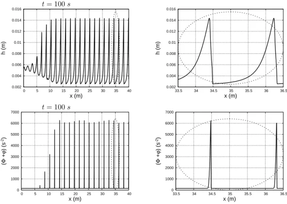
0.002 0.004 0.006 0.008 0.01 0.012 0.014 0.016 0 5 10 15 20 25 30 35 40 h (m) x (m) 0.002 0.004 0.006 0.008 0.01 0.012 0.014 0.016 33.5 34 34.5 35 35.5 36 36.5 h (m) x (m) 0 1000 2000 3000 4000 5000 6000 7000 0 5 10 15 20 25 30 35 40 ( Φ + ϕ ) (s -2) x (m) 0 1000 2000 3000 4000 5000 6000 7000 33.5 34 34.5 35 35.5 36 36.5 ( Φ + ϕ ) (s -2) x (m) t = 100 s t = 100 s

Figure 5: Case 2. The roll-waves formation (at the left) and a magnified view (at the right) are shown both for the wave profile and the enstrophy .

0.6 0.7 0.8 0.9 1 1.1 1.2 1.3 1.4 1.5 1.6 1.7 0 0.2 0.4 0.6 0.8 1 h/h 0 x/λ numerical results (RG) experimental results SV model 0 0.5 1 1.5 2 2.5 3 3.5 4 0 0.2 0.4 0.6 0.8 1 h/h 0 x/λ numerical results (RG) experimental results SV model CASE 1 CASE 2

Figure 6: Comparison of roll-wave profiles for model (1)-(3) (solid line), SV model (dashed line) with Brock’s experimental results (dots) for the Cases 1 and 2.

the wave envelope is about 40 m.

For the same value of the perturbation frequency ω = 2.0 [rad/s], the long-time solution to the Saint-Venant equations gives just a regular roll-wave train (Figure 9). The wave length of a single wave forming such a roll-wave train is 5 m.

Thus, the long-time behaviour of the model (1) – (3) results in a strongly modulated roll-wave train, while the Saint-Venant equations produce a regular wave train.

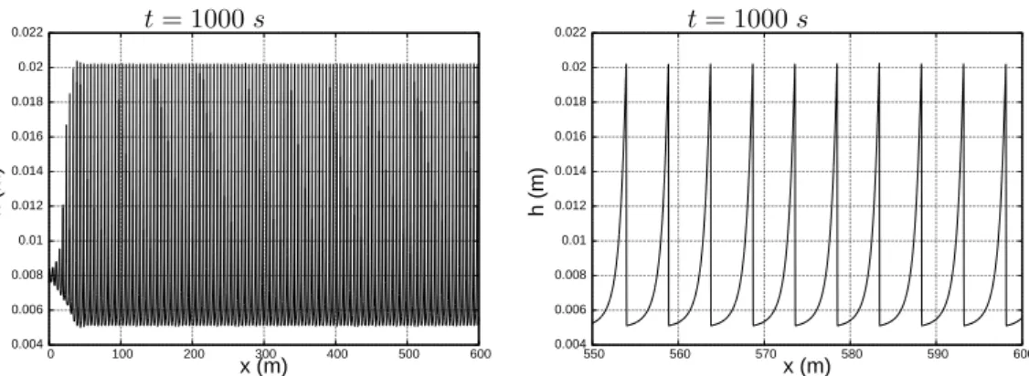
0.002 0.004 0.006 0.008 0.01 0.012 0.014 0.016 0 100 200 300 400 500 600 h (m) x (m) 0.002 0.004 0.006 0.008 0.01 0.012 0.014 0.016 550 560 570 580 590 600 h (m) x (m) t = 1000 s t = 1000 s

Figure 7: The profile of a roll-wave train for ω = 2.0 [rad/s] at the time instant 1000 s in the channel of 600 m long is at the left, and a magnified view is at the right. The other parameters correspond to Case 1. The length of a single roll wave is about 4 m. Number of cells is 60000. The roll-wave train is composed of single roll-waves having the same length and velocity. The wave amplitude is strongly modulated.

0 500 1000 1500 2000 2500 3000 0 100 200 300 400 500 600 ( Φ + ϕ ) (s -2) x (m) 0 500 1000 1500 2000 2500 550 560 570 580 590 600 ( Φ + ϕ ) (s -2) x (m) t = 1000 s t = 1000 s

Figure 8: The enstrophy of a roll-wave train for ω = 2.0 [rad/s] at the time instant 1000 s in the channel of 600 m long is at the left, and a magnified view is at the right. The other parameters correspond to Case 1. The length of a single roll wave is about 4.0 m. Number of cells is 60000. The roll-wave train is composed of single roll-waves having the same length and velocity. The wave enstrophy is strongly modulated.

4.2

Coarsening

If in the roll-wave train that propagates downstream there are waves of different lengths, they

begin to interact between them and coalesce. The short waves transfer their energy to long

waves, and finally a roll-wave train of a larger wavelength appears. This physical process is

called “coarsening”, or, as it was proposed by Brock [3], “growth by overtaking”. To observe the coarsening, we perturb at inlet the unstable uniform flow in the form

h(0, t) = h0(1 + a1sin(ω1t) + a2sin(ω2t))

with two different frequencies ω1, ω2 and amplitudes a1, a2. To a smaller frequency corresponds

a larger wavelength. Qualitatively, the scenario of “coarsening” does not depend too much on

exact values of ωi and amplitudes ai, i = 1, 2. For definiteness, we take ω1 = 6.06 [rad/s],

ω2= 4.55 [rad/s]. This corresponds to the wavelengths of 1.6 m and of 3.55 m, respectively. The

initial depth is h0= 0.01 m, the amplitudes are a2= 2a1= 0.1.

Two different development stages can be observed. The first one is a transition phase where a strong interaction between waves occurs and wave period starts to increase. In the second stage, a

0.004 0.006 0.008 0.01 0.012 0.014 0.016 0.018 0.02 0.022 0 100 200 300 400 500 600 h (m) x (m) 0.004 0.006 0.008 0.01 0.012 0.014 0.016 0.018 0.02 0.022 550 560 570 580 590 600 h (m) x (m) t = 1000 s t = 1000 s

Figure 9: A regular roll-wave train is formed when the Saint-Venant equations are used (at the left). The results are obtained for ω = 2.0 [rad/s] at the time instant 1000 s in the channel of 600 m long. A magnified view is at the right. The length of a single roll wave is about 5.0 m. Number of cells is 60000. The modulations are absent.

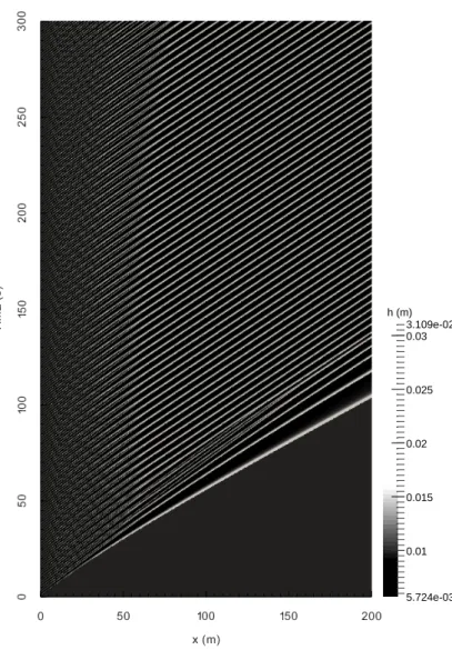
roll-wave train is formed with waves of constant length and velocity, with a strong non-stationary amplitude modulation (see Figure 10). The space-time diagram showing the coarsening process is shown in Figure 11. The trajectories of the roll-wave crests are shown by white lines. The coarsening corresponds to the intersection of these lines. It can be clearly seen in Figure 11, that near the right boundary of the computation domain, a permanent roll-wave train is formed. All the waves have the same lengths and velocities. Indeed, the crest trajectories become equidistant parallel straight lines. The coarsening process is achieved at the distance about 80 m. The non-stationary amplitude modulation does not change anything both in the wave train velocity and in the distance between neighbouring waves.

0.005 0.01 0.015 0.02 0.025 0.03 0.035 0 20 40 60 80 100 120 140 160 180 200 h(m) x(m) 0.005 0.01 0.015 0.02 0.025 0.03 0.035 0 20 40 60 80 100 120 140 160 180 200 h(m) x(m) 0.005 0.01 0.015 0.02 0.025 0.03 0.035 0 20 40 60 80 100 120 140 160 180 200 h(m) x(m) 0.005 0.01 0.015 0.02 0.025 0.03 0.035 0 20 40 60 80 100 120 140 160 180 200 h(m) x(m) 0.005 0.01 0.015 0.02 0.025 0.03 0.035 0 20 40 60 80 100 120 140 160 180 200 h(m) x(m) 0.005 0.01 0.015 0.02 0.025 0.03 0.035 0 20 40 60 80 100 120 140 160 180 200 h(m) x(m) t = 50 s t = 100 s t = 150 s t = 200 s t = 250 s t = 300 s

Figure 10: Coarsening in the long open channel with the following boundary conditions h(0, t) =

h0(1 + a1sin(ω1t) + a2sin(ω2t)), where the amplitudes of perturbations a1 = 0.05, a2= 2a1, the

frequencies ω1= 6.06 [rad/s], ω2= 4.55 [rad/s], h0= 0.01 [m]. Number of cells N = 20000. The

0.01 0.015 0.02 0.025 0.03 5.724e-03 3.109e-02 h (m)

Figure 11: The space-time diagram showing the coarsening in the long open channel of 200 m long. The trajectories of wave crests are shown by white lines. The coarsening corresponds to the intersection of these lines (left part of the computation domain ).

4.3

Periodic box

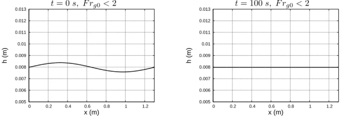
We partially repeat here the above numerical experiments for the periodic box. We take the initial sinusoidal perturbation of the free surface in the form given by (11). The amplitude of perturbation a is always 0.05. We will see how the perturbation evolves in time. As in the case of a long channel, one can show that the roll wave is not formed for the generalized Froude number smaller than two (Figure 12). For the generalized Froude number greater than two, one can see that just a single roll wave was formed (see Figures 13 for Case 1 and Case 2, respectively). The comparison of profiles of a single periodic roll wave with that measured by Brock is shown for the model RG (1)-(3) and for the SV equations. A good agreement between model (1)-(3) and Brock’s experiments can also be observed. As it was expected, the SV equations exaggerate both the wave amplitude and profile.

Let us show that final numerical solution does not depend on the form of the initial perturba-tion. We consider two different initial perturbations:

h(x, t)|t=0= h0(1 + a sin(8πx/Lb)) , 0≤ x ≤ Lb,

and

h(x, t)|t=0= h0(1 + 2a sin(4πx/Lb) + a sin (2πx/Lb)) , 0≤ x ≤ Lb.

For definiteness, we take Lb = 1.3 m corresponding to Case 1. At the time moment 100 s, we

obtain the same single wave of length Lb= 1.3 m (see Figure 14). In Figure 15 we present the

0.005 0.006 0.007 0.008 0.009 0.01 0.011 0.012 0.013 0 0.2 0.4 0.6 0.8 1 1.2 h (m) x (m) 0.005 0.006 0.007 0.008 0.009 0.01 0.011 0.012 0.013 0 0.2 0.4 0.6 0.8 1 1.2 h (m) x (m) t = 0 s, F rg0< 2 t = 100 s, F rg0< 2

Figure 12: Evolution of the numerical solution in the periodic box of Lb = 1.3 m . The generalized

Froude number is F rg0= 1.15 < 2, a = 0.05. The number of cells N = 1000. The roll-wave is not

formed as it was expected.

TEST h0[m] < h > [m] error

CASE 1 0.00798 0.007917 1 %

CASE 2 0.00533 0.0050327 5.5 %

Table 2: The average thickness of a single steady wave in a roll-wave train is shown for Case 1 and Case 2 in a long channel at the time instant 100 s. Compared to the periodic box, where the

average value must be exactly h0, the average value for a single steady wave in a roll-wave train

is a little bit smaller. However, as it can be seen from the Table, this error is small: 1% for Case

1, and 5.5% for Case 2. The error is defined as (h0− < h >)/h0.

average depth and the average discharge per unit width in the periodic box (Case 1), calculated in the following way:

< h > (t) = 1 Lb ∫ Lb 0 h(x, t)dx, < q > (t) = 1 Lb ∫ Lb 0 h(x, t)U (x, t)dx.

0.005 0.006 0.007 0.008 0.009 0.01 0.011 0.012 0.013 0 0.2 0.4 0.6 0.8 1 1.2 h (m) x (m) 0.002 0.004 0.006 0.008 0.01 0.012 0.014 0.016 0 0.2 0.4 0.6 0.8 1 1.2 1.4 1.6 1.8 h (m) x (m) 0 50 100 150 200 250 300 0 0.2 0.4 0.6 0.8 1 1.2 ( Φ + ϕ ) (s -2) x (m) 0 1000 2000 3000 4000 5000 6000 0 0.2 0.4 0.6 0.8 1 1.2 1.4 1.6 1.8 ( Φ + ϕ ) (s -2) x (m) 0.6 0.7 0.8 0.9 1 1.1 1.2 1.3 1.4 1.5 1.6 1.7 0 0.2 0.4 0.6 0.8 1 h/h 0 x/λ numerical results (RG) experimental results SV model 0 0.5 1 1.5 2 2.5 3 3.5 4 0 0.2 0.4 0.6 0.8 1 h/h 0 x/λ numerical results (RG) experimental results SV model t = 100 s t = 120 s t = 100 s t = 120 s CASE 1 CASE 2

Figure 13: Evolution of the numerical solution in the periodic box of 1.3 m (at the left) and 1.8 m long (at the right) with the parameter values corresponding to Case 1 and Case 2, respectively. Number of cells N = 1000. The numerical solution becomes stationary very rapidly.

The average depth conserves all the time. The discharge is not conserved. However, when a single wave is formed, the wave velocity becomes constant, so the average discharge becomes also constant. So, even if, a priori, the periodic box and the long channel problem are not equivalent, they becomes equivalent in the long time limit. This allows us to use the periodic box as a mathematical tool for the study of qualitative properties of long waves. Below we use the periodic box for the instability study of roll-waves.

0.005 0.006 0.007 0.008 0.009 0.01 0.011 0.012 0.013 0 0.2 0.4 0.6 0.8 1 1.2 h (m) x (m) 0.005 0.006 0.007 0.008 0.009 0.01 0.011 0.012 0.013 0 0.2 0.4 0.6 0.8 1 1.2 h (m) x (m) 0.005 0.006 0.007 0.008 0.009 0.01 0.011 0.012 0.013 0 0.2 0.4 0.6 0.8 1 1.2 h (m) x (m) 0.005 0.006 0.007 0.008 0.009 0.01 0.011 0.012 0.013 0 0.2 0.4 0.6 0.8 1 1.2 h (m) x (m) t = 0 s t = 100 s t = 0 s t = 100 s b) a)

Figure 14: The numerical solution in the periodic box does not depend on initial

pertur-bations. A single roll-wave of length 1.3 m was formed. Number of cells N = 1000,

F rg0 = 3.63. The initial conditions for each case for the depths was taken in the

fol-lowing form: a) h(x, t = 0) = h0(1 + a sin(8πx/Lb)) , 0 ≤ x ≤ Lb; b) h(x, t = 0) =

h0(1 + 2a sin(4πx/Lb) + a sin(2πx/Lb)) , 0≤ x ≤ Lb. 0.0078 0.0079 0.008 0.0081 0.0082 0.0083 0.0084 0.0085 0.0086 0 10 20 30 40 50 60 70 80 90 100 average values (m) time (s) average depth (m) average discharge (m)

Figure 15: Average depth and discharge in the periodic box of 1.3 m are shown. The flow

parameters correspond to Case 1. Number of cells N = 3000, F rg0= 3.63.

4.3.1 Wave instability in a periodic box

A periodic box of different lengths multiple of Lbis considered. In particular, Case 1 is considered

computations show that a single stable wave is formed until the box length 8 Lb. The wave is

morphologically stable ( it has always a steeply sloping wave front, then a continuous zone where the depth increases progressively, and finally, a slowly decreasing monotonic zone until reaching again the wave front). However, its amplitude changes slowly in time in the same way as in the

long channel where modulations of the roll-waves train appear. Beginning from the length 9 Lb

to 13 Lb this single wave becomes very non-stationary and it finally breaks into two waves for

the box of length 14 Lb. For the periodic box of 15 Lb we obtain three waves. The minimal

length of periodic box for which a single roll wave is stable, was not found. Analogous results were obtained for the SV equations (Figure 16, at the left). As for the long channel, the single stable waves for the SV equations, are steady : the amplitude modulations are not present. The critical “bifurcation” lengths are approximately the same for both models.

0.004 0.006 0.008 0.01 0.012 0.014 0.016 0.018 0.02 0.022 0 2 4 6 8 10 h (m) x (m) 0.005 0.01 0.015 0.02 0.025 0.03 0 2 4 6 8 10 12 14 h (m) x (m) 0.004 0.006 0.008 0.01 0.012 0.014 0.016 0.018 0.02 0.022 0 2 4 6 8 10 12 14 16 18 h (m) x (m) 0.004 0.006 0.008 0.01 0.012 0.014 0.016 0.018 0.02 0.022 0.024 0.026 0 2 4 6 8 10 12 14 h (m) x (m) 0.004 0.006 0.008 0.01 0.012 0.014 0.016 0.018 0.02 0.022 0 2 4 6 8 10 12 14 16 18 h (m) x (m) 0.004 0.006 0.008 0.01 0.012 0.014 0.016 0.018 0.02 0.022 0.024 0 2 4 6 8 10 12 14 16 18 h (m) x (m) 8 Lb, RG 11 Lb, SV 14 Lb, RG 12 Lb, SV 15 Lb, RG 15 Lb, SV

Figure 16: The instability scenario in the periodic box of different lengths multiple of Lb= 1.3 m

at the same time instant 1000 s. The parameters correspond to Case 1. Number of cells N = 4000 for all computations.

5

2D simplified model

5.1

Governing equations

Multi-dimensional model of shear shallow water flows is much more complicated. Its structure is reminiscent of equations of compressible turbulent flows [15], [11], [6]. Even if it is hyperbolic, it is not conservative. To avoid the treatment of non-conservative equations, we consider here a simplified model, where the complete Reynolds stress tensor is replaced by a spherical one. Such an approximation corresponds to the consideration of isotropic turbulence, often used in applications. The governing equations for the general case of a space varying topography are :

ht+ div(hU) = 0, (16)

(hU)t+ div{hU ⊗ U + pI} = −gh∇b − CU|U|, (17)

(hE)_t+ div{hUE + pU} = −Ce|U|3. (18)

Here z = b(x), x = (x, y)T _{is the bottom topography, the free surface is at z = b(x) + h(t, x),}

h(t, x) is the fluid layer thickness, U = (U, V )T _{is the average velocity, |U| =}√_U2_{+ V}2_{, and Ψ} is the enstrophy (squared vorticity). The total energy E and the “pressure” p are :

E =|U| 2 2 + gh 2 + gb + Ψh2 2 , p = gh2 2 + Ψh 3_.

As in the 1D case, the system implies the equation for the enstrophy: h3 2 DΨ Dt = (C− Ce)|U| 3_, where D Dt = ∂ ∂t+ U ∂ ∂x+ V ∂ ∂y. We decompose Ψ = Φ + φ,

where φ is a given small constant (describing the intensity of the vortexes in the boundary layer near the bottom), and Φ is the large scale enstrophy. The equations are written here in a reference system where the direction of gravity is orthogonal to the (x, y)-plane. This a little bit different from 1D case, where x-direction corresponds to the tangent vector of an inclined plane. However, for a little inclination angle, the equations are equivalent.

We take the bottom topography in the form b(x) =−x tan θ that corresponds to an inclined

plane. It is supposed that θ = const > 0. The system of conservation laws is reminiscent of the Euler equations of compressible fluids with a right-hand side. It is hyperbolic (cf. [10]). Due to the following obvious identity :

hD

Dtgb = gh (bt+ U bx+ V by) = ghU bx= ghU tan θ, the energy equation can be simplified to :

( h ˜E ) t + div { hU ˜E + ( gh2 2 + (Φ + φ)h 3 ) U } =−ghU∇b − Ce|U|3, (19)

where the modified total energy is : ˜ E = |U| 2 2 + gh 2 + (Φ + φ)h2 2 .

We will use here a multi-dimensional unsplit extension of the one-dimensional conservative Go-dunov scheme presented earlier. Our two-dimensional system (16), (17) and (19) can be rewritten in the following form :

Ut+ F(U)x+ G(U)y= S(U), (20)

where the vector of the “conserved” quantities U, the vectors of fluxes in x - direction F(U), in y - direction G(U), and the source terms vector S(U) are:

U =     h hU hV h ˜E     , F(U) =     hU hU2_{+ p} hU V hU ˜E + pU     , G(U) =     hV hU V hV2_{+ p} hV ˜E + pV     , S(U) =     0 g tan θh− CU(U2_{+ V}2₎1/2 −CV (U2_{+ V}2₎1/2 −Ce(U2+ V2)3/2+ g tan θhU,     , p = gh 2 2 + (Φ + φ)h 3_.

Consider a typical finite volume cell Ii,j = ∆x× ∆y. A finite volume scheme to solve the

homo-geneous part of system (20) is :

Un+1_i,j = Un_i,j+ ∆t ∆x [ F∗,n_i−1/2,j− F∗,n_i+1/2,j ] + ∆t ∆y [ G∗,n_i,j−1/2− G∗,n_i,j+1/2 ] .

Across each intercell boundary in each direction we solve the Riemann problem to find the

nu-merical fluxes F∗,n_i±1/2,j, G∗,n_i,j±1/2. The integration of the source term is done in the same way as

in 1D case. In particular, we show that a single roll-wave formation does not depend of transverse perturbations. We use the two-dimensional model for a periodic box of 1.3 m long in x-direction, and 0.1175 m width, with the initial conditions in the following form:

h|t=0= h0{1 + a sin(8πx/Lx) + a sin(8πy/Ly)} , U|t=0= U0, V|t=0= 0, Φ|t=0= 0,

where Lxand Ly are the length and the width of the periodic box, respectively. In the direction y

we use the wall boundary conditions. The parameters values correspond to Case 1. A single wave which is formed at the time instant 150 s corresponds to that obtain in one-dimensional case ( Figure 14).

Figure 17: The numerical solution of a simplified 2D model in a periodic box of 1.3 m long in x-direction, and of width 0.1175 m, for 400× 40 mesh is shown at the initial time instant (at the right) and at the time instant 150 s (at the left). A single stationary wave was formed. The final stationary solution does not depend on transverse perturbations.

6

Conclusion

The purpose of this work was the numerical study of the roll-waves that develop from a uniform unstable flow down an inclined rectangular channel. In particular, the formation of the roll-waves is studied by two different approaches. In the first approach, the roll-waves were generated in a long channel where the free surface was perturbed only at the channel inlet by a wave maker. The average discharge was fixed. In the second approach, the roll-waves were produced in a “periodic box” with a uniform flow velocity. The average depth of a perturbed free surface was the same as in the long channel.

First, the generation of a periodic roll-wave train was studied for a long channel for two sets of experimental parameters (noted as Case 1 and Case 2) corresponding to Brock’s experiments [3], [4]. In both cases, the free surface profile for the model (1)- (3) was found in a very good agreement with the experimental results, while the SV equations give a wrong wave form and amplitude Mathematical properties of the model were tested in the case where the perturbation frequency was much lower than the experimental one, so long waves were generated at the channel inlet. The amplitude and the enstrophy of the corresponding roll-waves train are strongly modulated, while the SV equations give for the same set of parameters a steady roll-wave train. In the case where the waves of two different lengths were generated at the channel inlet, the coarsening was observed, as it happens also for the SV equations. The coarsening phenomenon is always accompanied by a modulation phenomenon.

The formation of a single wave composing a roll-wave train in a “periodic box” was studied for the same sets of experimental parameters. The free surface profile for the model (1)- (3) was found also in a very good agreement with the experimental results. This allows us to justify the use of the “periodic box” as a simple mathematical tool for a qualitative study of roll-waves stability. In particular, we studied the stability of a single steady wave by taking its length as a multiple of

Lb= 1.3 m corresponding to Case 1 of Brock’s experiments. It was shown that the wave becomes

morphologically unstable after some critical wave length. This fact is also valid for the SV model. Finally, we proved that a single steady wave corresponding to Case 1 is stable under multi-dimensional perturbations in the framework of a model which represents a simplification of a general multi-D model of shear shallow water flows.

Our future work will certainly be oriented to the development of a full multi-dimensional model capable to describe more complex multi-dimensional non-stationary physical phenomena.

Several interesting phenomena were observed. First, it was proven that there exists Lmaxsuch

that any single roll wave of length L > Lmaxnot stable. This can help to generalise the analytical

results obtained by Liapidevskii ( modulational stability study) [2] and Barker et al. [1] (the

linear stability study) for the SV equations, to the case of the model (1), (2), (3). The minimal length of periodic box for which a single roll wave is stable, was not observed.

Second, a coarsening phenomenon was observed. When the inlet perturbation has two different frequencies, it produces the waves of different wavelengths. The waves begin to interact. The short waves transfer their energy to the long waves, and finally we obtain the train of roll waves of a larger wavelength. A strong non-stationary modulation of the wave amplitude was observed.

Finally, for a 2D simplified “Toy Model” we show that steady numerical solution corresponding to experimental data does not depend of transverse perturbations.

Acknowledgement

K. Ivanova and S. Gavrilyuk were partially supported by ANR BoND, France. The authors thank S. Hank, N. Favrie and J. Massoni for help with domain decomposition methods.

7

APPENDIX A

In this Appendix we will describe the higher-order extension of Godunov’s Method - MUSCL(“Monotonic Upstream-centred Scheme for Conservation Laws”) - Hancock method. The basic idea is to gen-eralize Godunov’s method by replacing the piecewise constant representation of the solution by a more accurate piecewise linear reconstruction. For model (1) - (3) we use the MinMod limiter for depth, velocity and “pressure”. This method involves three distinct steps to obtain a higher-order

i+1 i i+1/2 i+1 L U U UR L Ui+1 R i i

Figure 18: At each interface i+1/2 boundary extrapolated values UR

i and ULi+1are evolved to ¯URi

and ¯UL

i+1, to form the piecewise constant data for conventional Riemann problem at the intercell

boundary[16]. accurate scheme.

The first one is a reconstruction of data. Recall that Un_i represents an integral average in cell

Ii= [xi−1/2, xi+1/2] given by Uni = 1 ∆x

∫x_i+1/2 x_i−1/2 U(x, t

n_{)dx . Now we replace the constant states}

Un_i by piecewise linear functions Ui(x) :

Ui(x) = Uni +

x−xi

△x △i, x∈ [0, △x] (21)

where ∆i

∆x is a slope of Ui(x) in cell Ii (see Figure 18). The boundary extrapolated values are

given by

UL

i = Uni − ∆i/2; URi = Uni + ∆i/2. (22)

As to the choice of slopes ∆i we define here ∆i=1₂MinMod(∆Ui−1/2, ∆Ui+1/2), where

∆Ui−1/2≡ Uni − U

n

i−1, ∆Ui+1/2≡ Uni+1− U n i ,

and MinMod limiter is defined as :

MinMod(a, b) = 1₂(sgn(a) + sgn(b)) min(|a|, |b|). (23)

The second one is a prediction step, when we evaluate UL

i, URi at the instant ∆t/2. ¯ UL i = ULi + ∆t 2∆x[F(U L i)− F(URi )], ¯ UR i = U R i + ∆t 2∆x[F(U L i)− F(U R i )],

Figure 18 illustrates two first steps at the intercell boundary position i + 1/2. The boundary

extrapolated values UR

i , ULi+1 are evolved to ¯URi , ¯ULi+1. They form piece-wise constant data for a

conventional Riemann problem at the cell interface i + 1/2.

The third step is the resolution of the Riemann problem for the system :

with the initial condition : U(x, 0) = { _¯ UR i , x < 0, ¯ UL i+1, x > 0

To compute Godunov fluxes F∗,n_i+1/2 = F( ¯UR

i , ¯ULi+1) and F∗,ni−1/2 = F( ¯U

R

i₋₁, ¯ULi), we solve the

Riemann problems between i, i + 1 and i− 1, i cells correspondingly. For that we use the HLLC

Riemann solver. We use finally the Godunov scheme :

¯ Un+1_i = Un i −∆x∆t ( F∗,n_i+1/2− F∗,n_i−1/2 ) , (24)

where F∗,n_i+1/2 is the numerical flux function, which prescribes order of accuracy, with the time

average of the flux at the edge xi+1/2 of the cell. Note that taking ∆i ≡ 0 for all i and n recovers

first order Godunov’s method.

To integrate the source term, we use Strang’s splitting with a 4th_{order Runge – Kutta scheme.}

7.1

Order of convergence

To find the order of convergence, we construct a sequence of approximate solutions and then we calculate the error compared with a refined mesh solution (16000 cells). In Figure 19 one can see the convergence of MUSCL-Hancock scheme (MinMod limiter) with the line slope corresponding to approximately 1.4. We took here a periodic box of 1.3 m long to calculate error by the formula :

error = √

ΣN

i=1Σkj=1[H(i)− ˜H(k(i−1)+j)]

2

∆x Lb

Lb

.

Here N is the number of cells for the sequence of approximate solutions (100, 200, 400, 500, 1000, 2000,

4000 and 8000), k is obtained using the formula Nmax= kN , where Nmax= 16000 that correspond

to the numerical solution with a good refined mesh. H(i) is fluid depth in the cell i, ˜H(k(i−1)+j)

is the value of the fluid depth in the cell k(i− 1) + j for a good refined numerical solution.

-12 -11 -10 -9 -8 -7 -6 -5 -4 -3 -10 -9 -8 -7 -6 -5 -4 Ln(error) Ln(∆x/Lb ) numerical results line with slope 1.4

Figure 19: The order of convergence of the numerical method for the periodic box of 1.3 [m] with the data corresponding to the case 1. In this figure Ln(error) is represented as a function of the grid size with 100, 200, 400, 500, 1000, 2000, 4000 and 8000 mesh cells. The “exact solution” was replaced by a numerical solution with 16000 points. The 1.4 order convergence slope is shown with a continuous line.

References

[1] B. Barker, M. A. Johnson, P. Noble, L. M. Rodrigues, and K. Zumbrun.

Sta-bility of viscous st.venant roll-waves : from onset to infinite-froude number limit.

[2] A. Boudlal and V. Yu. Liapidevskii. Stabilit´e de trains d’ondes dans un canal d´eecouvert. CRAS M´ecanique, 330(2-3):291–295, 2002.

[3] R. R. Brock. Development of roll waves in open channels. 1967, PhD Thesis, Caltech. [4] R. R. Brock. Development of roll-wave trains in open channels. Journal of the Hydraulics

Division, 95(4):1401–1428, 1969.

[5] R. F. Dressler. Mathematical solution of the problem of roll-waves in inclined opel channels. Communications on Pure and Applied Mathematics, 2(2-3):149–194, 1949.

[6] S. L. Gavrilyuk and H. Gouin. Geometric evolution of the reynolds stress tensor. International Journal of Engineering Science, 59:65–73, 2012.

[7] S. K. Godunov. A difference method for numerical calculation of discontinuous solutions of the equations of hydrodynamics. Matematicheskii Sbornik, 89(3):271–306, 1959.

[8] R. J. LeVeque. Numerical methods for conservation laws, volume 132. Springer, 1992. [9] V. Yu. Liapidevskii and V. M. Teshukov. Mathematical models for a long waves propagation

in an inhomogeneous fluid. 2000, (in Russian).

[10] L. V. Ovsyannikov. Lectures on the Fundamentals of Gas Dynamics. Moscow, Nauka, Russia, 1981 (in Russian).

[11] G. L. Richard. Elaboration d’un mod`ele d’´ecoulements turbulents en faible profondeur:

appli-cation au ressaut hydraulique et aux trains de rouleaux. PhD thesis, Aix-Marseille, 2013. [12] G. L. Richard and S. L. Gavrilyuk. A new model of roll waves: comparison with brock’s

experiments. Journal of Fluid Mechanics, 698:374–405, 2012.

[13] G. L. Richard and S. L. Gavrilyuk. The classical hydraulic jump in a model of shear shallow-water flows. Journal of Fluid Mechanics, 725:492–521, 2013.

[14] G. Russo. Central schemes for conservation laws with application to shallow water equations. In Trends and Applications of Mathematics to Mechanics, pages 225–246. Springer, 2005. [15] V. M. Teshukov. Gas dynamics analogy for vortex free-boundary flows. Journal of Applied

Mechanics and Technical Physics, 48(3):303–309, 2007.

[16] E. F. Toro. Riemann solvers and numerical methods for fluid dynamics: a practical introduc-tion. Springer Science & Business Media, 2009.

[17] H. Tougou. Stability of turbulent roll-waves in an inclined open channel. Journal of the Physical Society of Japan, 48(3):1018–1023, 1980.

[18] B. Zanuttigh and A. Lamberti. Roll waves simulation using shallow water equations and weighted average flux method. Journal of Hydraulic Research, 40(5):610–622, 2002.