HAL Id: hal-01494475
https://hal.sorbonne-universite.fr/hal-01494475
Submitted on 23 Mar 2017HAL is a multi-disciplinary open access
archive for the deposit and dissemination of sci-entific research documents, whether they are pub-lished or not. The documents may come from teaching and research institutions in France or abroad, or from public or private research centers.
L’archive ouverte pluridisciplinaire HAL, est destinée au dépôt et à la diffusion de documents scientifiques de niveau recherche, publiés ou non, émanant des établissements d’enseignement et de recherche français ou étrangers, des laboratoires publics ou privés.
Ménard
To cite this version:
Christophe Dumouchel, Wojciech Aniszewski, Trung-Thanh Vu, Thibaut Ménard. Multi-Scale Anal-ysis of Simulated Capillary Instability. International Journal of Multiphase Flow, Elsevier, 2017, 92, pp.181-192. �10.1016/j.ijmultiphaseflow.2017.03.012�. �hal-01494475�
ACCEPTED MANUSCRIPT
2
Multi-Scale Analysis of Simulated Capillary Instability
Christophe Dumouchel1, Wojciech Aniszewski2, Trung-Thanh Vu1, Thibaut Ménard1
1
CORIA – UMR 6614
Normandie Université, CNRS UMR 6614 - CORIA, Université et INSA de Rouen Avenue de l’Université, BP 12
76801 Saint-Etienne-du-Rouvray, FRANCE
2
Sorbonne Universités, UPMC Université Paris 06, CNRS UMR 7190 Institut Jean Le Rond d'Alembert
75005 Paris, France
Abstract
This paper presents the 3-D multi-scale analysis of a cylindrical liquid ligament subjected to a capillary instability. This analysis aims to investigate the evolution of the ligament interface paying a specific attention to the physical mechanisms involved at small scales. The capillary instability behavior is obtained from direct numerical simulations. Calculations are performed for several wavenumbers of the initial sinusoidal perturbation. During the capillary instability, the scale space is divided in two regions: the small-scale region where a thinning mechanism is identified and the large-scale region where a thickening mechanism is observed. Although the characteristic scale dmax of the large-scale region displays a dynamics that agrees with the
Rayleigh linear theory, this agreement is lost for the characteristic scale d1of the small scale
region showing that the non-linear effects mainly concentrate on the small scales. The dynamics of the characteristic scale d1 follows three successive regimes. The development of
ACCEPTED MANUSCRIPT
3
a simple model allows identifying the physical mechanisms related to these three regimes as well as their dependences with the wavenumber of the perturbation. Among other results it is found that the capillary contraction regime that develops when the breakup is approached is always preceded by an elongation mechanism whose effect is to increase the specific-surface-area of the ligament.
Keywords: Multi-scale analysis; two-phase flow; direct numerical simulation; capillary
ACCEPTED MANUSCRIPT
4
1 Introduction
Liquid atomization processes, which designates the deformation and breakup of a free liquid flow evolving in a gaseous environment, need specific investigations to be better understood and modelled. From an experimental point of view, the most common approaches to investigate these processes are based on image analysis (Dumouchel, 2008). Several characteristics are measured, i.e., the breakup length, the wavelength of perturbations, the size of liquid fragments or the diameter of droplets, etc. Despite of their physical relevance, these characteristics provide a split-up description of the process.
The atomization of a liquid flow is a matter of energy exchange between the liquid-gas interface and the two fluids: the variation of the interface area is associated with energy transfer. Creation of interface requires energy, and inversely, interface reduction provides energy (Evers 1994). The liquid-gas surface stores energy, which, per unit mass, is equal to the product of the specific-surface-area (surface area per unit mass) and the surface tension (Evers, 1994). The specific-surface-area is conveyed by the shape of the liquid system. During an atomization process, this shape varies in a complex way. As example of this can be seen in Fig. 1 that shows the temporal evolution of an atomizing liquid ligament. Its deformation produces liquid swells and threads. The thickening of the ligament into swells is accompanied by a local reduction of the specific-surface-area (IR in Fig. 1) since the sphere ensures the smallest interface area for a given liquid volume. On the other hand, the thinning of threads locally increases the specific-surface-area (IC in Fig. 1). This demonstrates that events of interface reduction and creation occur at the same time but at different scales. Thus, a multi-scale approach is recommended to investigate liquid atomization processes. The scale distribution introduced in previous works (Dumouchel and Grout 2009, 2011; Dumouchel et al. 2015a, 2015b) is a possible alternative to achieve this.
ACCEPTED MANUSCRIPT
5
The notion of scale-distribution is inspired from the Euclidean Distance Mapping method to measure fractal dimension (Bérubé & Jébrak 1999). The cumulative scale distribution En(d)
measures the relative amount of the liquid system lost after the application of an erosion operation at scale d. The derivative in the scale space of this cumulative (dEn(d)/dd) is the
scale-distribution en(d). In 3-D (n = 3), the scale distribution represents the surface area of the
eroded system divided by twice the total volume of the system. For d = 0, this quantity is identical to the specific-surface-area introduced by Evers (1994).
The application of the scale distribution to investigate a liquid atomization process has been presented in several works (Dumouchel and Grout 2009, 2011; Dumouchel et al. 2015a, 2015b). The 2-D scale distribution, obtained by analyzing images of the atomization processes, evolves continuously during the flow deformation and fragmentation (Dumouchel and Grout 2009). The modeling of the temporal evolution of this distribution can be approached by the scale entropy diffusion model (Dumouchel and Grout 2009, 2011; Dumouchel et al. 2015b). Recently, the multi-scale analysis succeeded in identifying the physical mechanisms involved in the atomization of stretched ligaments emanating from turbulent liquid sheets (Dumouchel et al. 2015a). In particular that work shows that the presence of an elongation mechanism of the small structures is beneficial in terms of small drop production. The mechanisms controlling the interface evolution at small scales are therefore important and should be explored in detail.
The present work aims to make use of the concept of scale distribution to investigate a deforming liquid system paying a specific attention to the mechanism involved at small scales. The fundamental case of a cylindrical ligament of liquid subject to a capillary instability isconsidered. Three main reasons motivated this choice. First, this instability has been widely studied as reported by the review articles due to Bogy (1979), Eggers (1997), Eggers and Villermaux (2008), Ashgriz and Yarin (2011). The advanced knowledge of the
ACCEPTED MANUSCRIPT
6
physics of this instability may turn out to be useful in the present approach. Second, the capillary instability can be obtained from direct numerical simulation instead of experiments. This allows a perfect control of the operating conditions. Third, since cylindrical ligaments are unstable for axisymmetric disturbances only, a 3-D scale analysis is possible. As noted above this allows us having access to the specific-surface-area of the system.
The elements of the multi-scale analysis are introduced in Section 2. Section 3 presents a review of the capillary instability as well as the results of the present simulation work. The multi-scale analysis is described in Section 4.
ACCEPTED MANUSCRIPT
7
2 The multi-scale description
The multi-scale analysis describes the liquid system by the cumulative scale function En(d)
where d is the scale of observation. This function is obtained by applying successive erosion operations to the liquid system. An erosion operation is illustrated in Fig. 2 for a 2-D system. Figure 2-left shows the initial system, which has a 2-D total surface area noted S2T. The
system is eroded by circular structuring elements with a diameter d. The eroded system (dark-gray area in Fig. 2-right) has a surface area noted S2(d). The erosion operation is applied for d
varying from 0 to infinity and the cumulative surface-based scale distribution E2(d) is
constructed as:
T T S d S S d E 2 2 2 2 (1)When d increases, E2(d) monotonously increases from 0 to 1. The first derivative of E2(d)
with respect to the scale is the surface-based scale distribution e2(d):
T S d L d d E d e 2 2 2 2 d d (2)This derivative is equal to the ratio of the perimeter length L(d) of the eroded system at scale d on twice S2T.
The extension of this definition in 3-D is straightforward. In this case, the system is characterized by its total volume VT, the erosion operation is performed with a sphere of
diameter d and the cumulative volume-based scale function E3(d) involves the volume V(d) of
ACCEPTED MANUSCRIPT
8
T T V d V V d E3 (3)The first derivative of E3(d) is the volume-based scale distribution e3(d). This function is
equal to the ratio of the 3-D surface area S3(d) of the eroded system divided by twice the
system total volume:
T V d S d d E d e 2 d d 3 3 3 (4)The distributions en(d) (n = 2, 3) are monotonously decreasing functions, their dimension is
the inverse of a length, and, being the derivative of a cumulative function, they are
normalized, i.e.,
d 1 0
d den . Note that e3(0) corresponds to the specific-surface-area
introduced by Evers (1994). Therefore, e3(d) can be seen as a generalization at all scales of
this concept.
When the liquid system is subject to a deformation, all functions introduced above become dependent on time t except the total volume VT. Therefore, the temporal evolution of e3(d,t)
always reflects a variation of the surface S3(d,t) (Eq. (4)) whereas the temporal evolution of e2(d,t) combines variations of the functions L(d,t) and S2T(t) (Eq. (2)).
For simple systems, mathematical expressions for the scale distribution en(d) can be
established. This is the case for a cylinder of diameter D and length L and a sphere of diameter D. As far as the cylinder is concerned, its lateral surface is considered only, i.e., the two circular ends are not counted as interface. The scale distributions of these systems are:
ACCEPTED MANUSCRIPT
9
D d d e D d D d D n d e D D d d e D d D d D n d e D n n n n n n for 0 ; for 1 : diameter of Sphere for 0 ; for 1 1 : diameter of Cylinder 1 2 (5)where n = 2 and 3 corresponds to the 2-D and 3-D description, respectively. In 2-D (n = 2 in Eq. (5)), the scale distribution of the cylinder is independent of d whereas the one of the sphere linearly depends on d. In 3-D (n = 3 in Eq. (5)), the scale distribution of the cylinder is linear and the one of the sphere is a second order polynomial. We see that the scale distribution discriminates cylinders from spheres. This feature is interesting in the context of liquid atomization processes where cylinders (ligaments) and spheres (drops) are frequently encountered objects. Note also that the diameter D of these systems is equal to the maximum scale dmax defined as the smallest scale for which en(d) = 0.
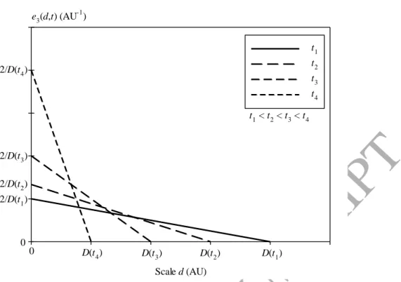
The mechanisms of interface variation at small scales in liquid atomization processes often involve liquid-thread thinning. It is therefore instructive to consider the case of a thinning cylindrical ligament, i.e., a cylinder with a diameter D(t) that decreases with time. The temporal evolution of the scale distribution e2(d,t) and e3(d,t) calculated from Eq. (5) are
shown in Figs. 3-a and 3-b. The scale distributions e2(d,t) are successive step functions
whereas the scale distributions e3(d,t) are successive linear functions. As t increases, the
characteristic features of this mechanism are a continuous increase of e2(d,t), a continuous
decrease of the scale derivative de3
d,t dd and a scale independence of these two functions. We note also that the width of both distributions decreases with time as imposed by the diameter D(t) and that the specific-surface-area continuously increases.ACCEPTED MANUSCRIPT
10
Combining the quasione-dimensional continuity equation provided by Stelter et al. (2000) together with the fact that the section of the cylinder is constant along the axial direction z, we obtain the rate of stretching , i.e.:
t
t D t D z v d d 2 (6)where v designates the longitudinal velocity. Considering Eqs. (5) and (6), we can express the stretching rate of the thinning cylinder as a function of the scale distributions:
e
d t t d e t d e t d e , ' , ' , , 2 3 3 2 2 (7)where the dot indicates a temporal derivative and the prime a scale derivative. The stretching rate is therefore independent of the scale d.
From a physical point of view, the thinning of a liquid ligament can be due to an elongation mechanism or a contraction mechanism. In the first case, the ligament is elongated by an external constraint and its volume is constant. In the second case, the contraction is driven by surface tension forces and expulses liquid out of the ligament whose volume therefore decreases. If for both mechanisms the specific-surface-area increases, the absolute amount of surface area actually increases during the elongation and decreases during the contraction. In the second case, the reduction of the ligament diameter is not compensated by an increase of its length. Both mechanisms are associated to a positive stretching rate and the only way to dissociate them from each other is to get an information on the temporal variation of the ligament volume.
ACCEPTED MANUSCRIPT
11
3 Capillary instability of liquid ligaments
3.1 General considerationsThe capillary instability manifests on a cylindrical ligament subjected to disturbances that induce surface displacements and generate a gradient of surface tension forces. Under certain conditions, the pressure distribution caused by these gradients generates internal flows that concentrate the liquid in certain regions to the detriment of others and rearrange the ligament as a succession of crests and necks. This process continues until the ligament diameter at the necks is so small that a breakup occurs and produces one drop for each swollen region. Complete reviews on the investigations dedicated to this topic are available in the literature (Bogy 1979; Eggers, 1997; Eggers & Villermaux 2008; Ashgriz & Yarin 2011). General considerations useful for the present investigation are considered hereafter.
The long wavelength initial perturbations are those for which the instability is triggered since they induce a reduction of the interface-surface-area and are therefore favored by surface tension (Plateau, 1849). The temporal linear-theory developed by Rayleigh (1878) demonstrates that only axisymmetrical surface perturbations are unstable and that their growth is exponential in time. Thus, the crest and neck diameters, Dc and Dn respectively, vary as:
t t D t D t t D t D L n L c 8 exp 2 8 exp 2 0 0 0 0 (8)where DL0 is the non-perturbed ligament diameter, t =
3 0
L
LD is the capillary time (L is the liquid density and is the surface tension) and is the non-dimensional temporal growth-rate that is given by:
ACCEPTED MANUSCRIPT
12
2 0 1 2 1 k k k I k I (9)In Eq. (9), k is the non-dimensional wavenumber of the perturbation; k = DL0/ (is the
wavelength of the perturbation) and I0 and I1 are the modified Bessel functions. Equation (9)
says that perturbations are unstable for k < 1, i.e., for greater than the ligament circumference and that the maximum growth rate = 0.343 occurs at k = 0.696.
The linear theory does not provide a complete description of the capillary instability and non-linear effects are often important. They induce an asymmetrical development of the initial sinusoidal perturbation (Yuen 1968) as well as time-dependent growth-rates for the neck and crest diameters (Goedde and Yuen 1970). When the breakup is approached the non-linear effects cause a pressure gradient in the axial direction such that the flux of fluid out of the neck is smaller than the flux into the swell causing a contraction between the neck and the swell and favoring the formation of a liquid thread that turns into a satellite droplet between two primary droplets (Goedde and Yuen 1970). This mechanism is enhanced when the wavenumber decreases. These non-linear effects and their dependence with the wavenumber were experimentally evidenced (Ruthland and Jameson, 1971; Pimbley and Lee, 1977; Vassallo and Ashgriz, 1991). The most relevant parameters controlling the formation of the satellites are the amplitude and the wavelength-to-diameter ratio of the initial perturbation. Numerical simulations of the capillary instability due to Ashgriz and Mashayek (1995) confirmed these results. In particular they reported that the size of the satellite decreases when the wavenumber or the initial amplitude of the perturbation increases.
ACCEPTED MANUSCRIPT
13
On the other hand the question of the dynamics of the pinch-off mechanism occurring just before the breakup event has been widely addressed. This contraction mechanism driven by surface tension forces raises two main difficulties that are due to the local decrease to zero of the ligament diameter. From a theoretical point of view, the Navier-Stokes equation forms a singularity. From an experimental point of view, the measurement of the pinch-off diameter is difficult all the more so since it decreases faster and faster as the breakup is approached. The results provided by theoretical scaling arguments (Eggers 1993; Eggers and Dupont 1994, Lister and Stone 1998), experimental investigations (Kowalewski 1996, Brenner et al. 1997, Amarouchene et al. 2001) and numerical models and simulations (Papageorgiou 1995, Brenner et al. 1997) conclude that successive dynamic regimes exist during the pinch-off mechanism, i.e., an inertia regime and a visco-capillary regime. The inertia regime occurs first when the dominant resistance against surface tension stems from the inertia of accelerating fluid elements. The resulting dynamic of the pinch-off diameter writes (Lister and Stone 1998):
2 13 t t D L L (10)Second, as the ligament diameter decreases, the visco-capillary regime manifests when the dominant resistance against surface tension stems from viscous forces. The resulting dynamic of the pinch-off diameter becomes (Lister and Stone 1998):
t t D L L (11)ACCEPTED MANUSCRIPT
14
3.2 Numerical Simulations and Results
For the numerical solution of the flow, the momentum conservation equations of Navier and Stokes are taken in the following form:
s
T p t u u u u I n u . 1 . (12)where u = (u,v,w) is the velocity field, and and µ stand for the local density and dynamic viscosity, respectively. Pressure is designated by p with I representing an identity tensor. The last term on the right-hand side is the surface tension force, thus naturally n designates the vector field normal to the interface S, κ is the curvature and the restriction of the force to the interface is ensured by the Dirac distribution δs centered at S. For all calculations presented in
this work, body forces are assumed zero and thus do not appear in Eq. (12). Note that Eq. (12) is presented in so-called one-fluid formulation (Tryggvason et al., 2011). Thus, due to two phases being present there is a discontinuity (jump) in , p and μ at the interface S which is how the surface tension force emanates. The flow is incompressible, thus the continuity equation is employed:
0
.u (13)
The flow Eqs. (12-13) are solved using the Archer 3D solver developed at the CORIA laboratory. It is a MAC (Marker-and-Cell) type solver using staggered, uniform grids. Initially written by Tanguy and Berlemont (2005) with DNS (Direct Numerical Simulation) of multiphase flows in mind, the code has since been successfully applied to model atomization
ACCEPTED MANUSCRIPT
15
(Ménard et al. 2007; Berlemont et al. 2013), turbulent mixing and evaporation (Duret et al. 2012) or instabilities (Aniszewski et al. 2014).
Archer solves Eq. (12) by a well-established projection method (Tryggvason et al. 2011), meaning that the equation is first solved by assuming zero pressure, finding an intermediate solution and correcting it using Eq. (13) in the process. As one of the stages of the projection method, Poisson equation for the pressure field has to be solved; this is done using the Multigrid method with conjugate gradients (MGCG; Brandt, 1984). All derivatives, except the ones concerning the level set method as described below, are discretized using second order finite differences, with standard set of boundary conditions available. For the work presented here, symmetric boundary condition is used in all directions, and 1/8th of the liquid cylinder is simulated.
Interface S is represented as a zero-level of the Level-Set function, in the framework of a method of the same name (Osher and Sethian, 1988; Osher and Fedkiw, 2001). As it is a passive scalar, its material derivative vanishes:
0 . t u (14)
which is to say that is passively advected with the flow. The level-set is a continuous distance function, i.e. it is, for an argument x, equal to the minimum distance between x and S. Continuity of makes Eq. (14) relatively easy to solve numerically: it can be done by representing spatial derivatives with chosen numerical scheme (in this work, the scheme is Weighted Essentially Non-Oscillatory, or WENO (Shu, 1997)). This means that the LS (Level Set) method evades the issues found in other interface tracking methods that employ discontinuous functions, such as VOF (Volume of Fluid). One example of such an issue is the efficiency in interfacial curvature calculation, leading to the phenomenon of numerically
ACCEPTED MANUSCRIPT
16
induced spurious currents (Aniszewski et al., 2014). Solution of the temporal progression of Eq. (14) is fully coupled with the temporal scheme for Eq. (12) using a 3rd order Runge-Kutta scheme. As the function is known to lose the distance property |∇| = 1 far from the zero level = 0 a redistancing procedure is correcting this by solving additional correction equation (Osher and Fedkiw, 2001).
The method used to trace the interface is important in that it is used for multiple purposes in a numerical setup. First, the surface tension force term of Eq. (12), σnκδs has all its variables
(except constant σ) calculated from the function, most notably the curvature κ. Second-order accurate curvature computation is possible with LS method, which is of fundamental importance when simulating a surface-tension driven flow. Secondly, it is used to calculate the pressure jump over the interface, and, in the framework of the Ghost Fluid Method (Fedkiw et al. 1999), enables differentiation close to the interface. This is possible as the carrying strict distance information, can be used to extrapolate e.g. velocity values from within one phase to the other in close vicinity of the interface (several grid-points).
An inherent shortcoming of the LS method is that it is prone to the ``loss of traced volume'' phenomenon (Tryggvason et al., 2011; Aniszewski et al., 2014), which is to say the information about small interfacial formations (small drops few grid-points across, thin films) is lost due to the lack of resolution in solution of Eq. (14). This is why in other applications of the Archer3D solver, CLSVOF (Coupled Level-Set Volume of Fluid) method of Sussman (Sussman and Puckett, 2000; Aniszewski et al., 2014) is used to impose mass conservation. However, in simulations of the Plateau-Rayleigh instability presented here, CLSVOF is not employed as the mass loss phenomenon does not occur - the simulations are halted once liquid breakup occurs.
All the simulations have been performed using a 128x128 resolution in directions parallel to cylinder radius and 256 points along the cylinder axis. The time step has been computed using
ACCEPTED MANUSCRIPT
17
the CFL condition based on convection, viscosity, gravity and capillary force using the method of Kang et al. (2000).
The simulations are conducted for ligaments of water (L = 1000 kg/m3; = 0.07 N/m,
µL = 0.001 kg/(ms)) into air. The initial ligament diameter is Dj = 666 µm corresponding to a
capillary time t = 2 ms and to an Ohnesorge number Oh = µL/(LDj)0.5 = 0.0065. The
amplitude of the initial sinusoidal perturbation is kept constant, i.e., 0 = 17 µm
(0/Dj = 0.025). Eight values of the non-dimensional wavenumbers k are considered, namely,
0.55; 0.60; 0.65; 0.69; 0.75; 0.80; 0.88 and 0.95.
The simulation result for k = 0.55 is shown in Fig. 4. The evolution of the ligament from t = 0 to the breakup time tBU (= 8.13 ms for this case) undergoes three distinct steps. First (left
column in Fig. 4), the ligament deformation increases in amplitude keeping a sinusoidal shape. Second (middle column in Fig. 4), the deformation of the ligament is not sinusoidal anymore. Two necks appear and a liquid thread develops between the main swells. Third (right column in Fig. 4), the necks do not travel anymore: they impose a local high-pressure that induces a pinch-off mechanism until breakup occurs.
These three steps are observed for every wavenumber k. The main differences concern their time duration and the shape of the system at breakup time tBU. Figure 5 shows the ligaments at
tBU for all wavenumbers. The images are on scale with each other and their width represents
/2. For the present working conditions, we note that a liquid thread is always formed. This means that a satellite droplet is always produced. When the wavenumber increases, the length and size of this thread decrease meaning that the size of the satellite droplet decreases. These behaviors agree with those reported by Ashgriz and Mashayek (1995) for their case Oh = 0.005 (Re = 1/Oh = 200 in their paper) and 0/Dj = 0.05 which is the closest to ours.
ACCEPTED MANUSCRIPT
18
parenthesis) where tBUtheo is the breakup time predicted by the linear theory (Rayleigh, 1878).
This time is reached when the neck diameter Dn is equal to zero. According to Eq. (8), tBUtheo
is given by: 0 2 ln 8 1 j BUtheo D t t (15)
where is calculated from Eq. (9). When k increases, tBU decreases and then increases, but
the smallest tBU is not obtained for k = 0.69 as reported by the linear theory but for k = 0.75.
The difference between tBU and tBUtheo is a manifestation of non-linear effects. Globally
speaking tBU > tBUtheo indicating that these effects slow down the process. Furthermore, as
noticed above from the size and the length of the liquid thread, the breakup time underlines the decreasing influence of the non-linear effects when k increases.
ACCEPTED MANUSCRIPT
19
4 Multi-scale analysis
4.1 The scale distributionsThe measurements of the surface-based cumulative distributions E2(d,t) are performed with
the software ImageJ from images similar to those shown in Figs. 4 and 5. The spatial resolution of these images is high (between 0.28 to 0.51 µm/pixel according to k). For this reason, the scale increment in the successive erosion operations is taken equal to 8 pixels. The calculation of the distribution e2(d,t) from the cumulative distribution E2(d,t) (see Eq. (2)) is
performed with a Scilab routine. This routine also corrects e2(d,t) in the small-scale region
where non-physical results are frequently obtained since erosions performed at small scales with ImageJ lacks accuracy. This distribution is expected to be linear in the small-scale region. In the present measurements, this linear behavior is always observed in the [50; 100 pixel] scale range and the correction consists in extending it to d = 0. For the determination of the volume-based distribution, the liquid ligament is assumed axisymmetric at all times. This assumption is reasonable in the present context because axisymmetric disturbances are unstable only. The distributions e3(d,t) is directly calculated from ImageJ and
do not require any correction in the small-scale range. For each value of k, the time dependent scale distributions en(d,t) are obtained from the analysis of several hundreds of images
(between 200 and 600 according to k).
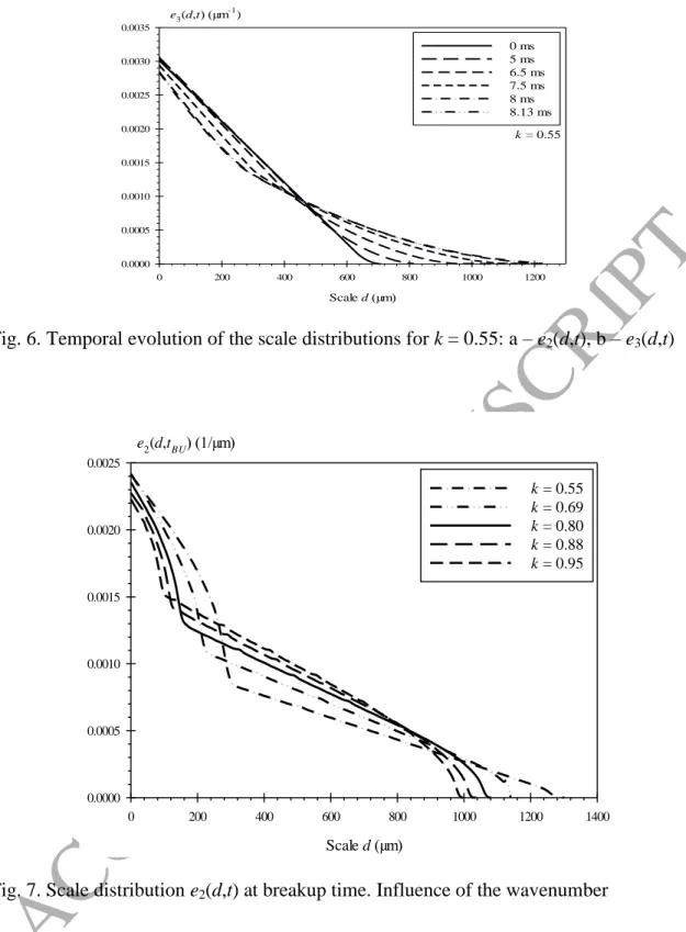
Figure 6 presents the distributions en(d,t) for k = 0.55: the surface-based scale distribution
e2(d,t) is shown in Fig. 6-a and the volume-based scale distribution e3(d,t) in Fig. 6-b. These
figures show a thickening mechanism at large scale and a thinning mechanism at small scales. The thickening mechanism is recognized by a continuous increase of the maximum scale dmax.
Defined as the smallest scale for which en(d,t) = 0, this scale is equal to the crest diameter of
ACCEPTED MANUSCRIPT
20
large-scale region (between 400 and 1200 µm in this case). According to Eq. (5), this indicates that the swollen part of the ligament is spherical. This observation actually depends on the wavenumber as illustrated in Fig. 7 where e2(d,tBU) is plotted for five wavenumbers.
We see that as k increases, the linear behavior of e2(d,tBU) in the large-scale region doesn’t
extent to the maximum scale. Therefore, at tBU, the large structure is less spherical when k
increases. This corresponds to what Fig. 5 shows.
The thinning mechanism at small scale is recognized by the continuous temporal increase of e2(d,t) or a continuous temporal decrease of e3'
d,t in this region (see Section 2).Furthermore, since e2(d,t) and e3'
d,t are both independent of the scale, this mechanism issimilar to the thinning of a cylindrical ligament (see Fig. 3-a and 3-b). The largest scale d1(t)
concerned by this mechanism is introduced. It is defined as the smallest scale for which e2(d,t)
stops increasing with time or e3'
d,t stops decreasing with time. Therefore d1(t) is thesmallest scale for which e2
d,t e3'
d,t 0. We see in Fig. 6 that d1(t) decreases with time. Figure 6-b shows that the specific-surface-area e3(0,t) globally decreases over the wholeprocess. This decrease is found for every k as shown in Fig. 8 which plots e3(0,0) and e3(0,tBU)
versus the wavenumber. The dots are the results obtained from the present simulations and the lines are the results obtained from the linear theory. For the latter case, e3(0,tBU) is calculated
by supposing that the perturbation is still sinusoidal at breakup and that its amplitude is equal to the radius of the ligament, paying attention that the volume is well conserved. The simulated and theoretical results report a decrease of the specific-surface-area of the ligament at breakup which is a known characteristic feature of the capillary instability. We see that this decrease is less when the wavenumber increases. Furthermore, whereas for k > 0.7 the simulated and theoretical results are in agreement, the reduction of the simulated specific-surface-area is less than the theoretical one for k < 0.7. Being a manifestation of the non-linear
ACCEPTED MANUSCRIPT
21
effects, this result says that these effects limit the decrease of the specific-surface-area and that they are negligible for high wavenumbers.
4.2 Characteristic scales and elongation rate
The dynamics of the characteristic scales dmax and d1 are examined in this section. Being
defined as the smallest scale for which en(d,t) = 0, dmax is also the smallest one for which
En(d,t) = 1. It is determined here as the smallest scale that satisfies the condition
E2(d,t) >0.999. Figure 9 shows the temporal evolution dmax(t) obtained for four wavenumbers.
After a time delay at least equal to 2 ms, the scale dmax reports an exponential increase with
time which writes:
t t D d m m j 8 exp 2 1 max (16)
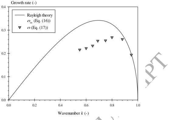
This equation is similar to Eq. (8) which makes sense since dmax(t) and Dc(t) are identical by
definition. Examples of the mathematical fit are shown in Fig. 9. The parameters m and m
are calculated for every k and reported in Table 1. The delay of the exponential behavior results in an initial amplitude smaller than the one imposed by the simulation. However, the temporal growth rates m are found to agree very well with those predicted by the linear
theory (see Fig. 10). Note however in Fig. 9 that for k = 0.95, dmax slightly deviates from the
exponential growth when the breakup time is approached.
The scale d1(t) is the smallest scale for which e2
d,t e3'
d,t 0. We see in Fig. 11 thatthese two equations are satisfied for the same scale. In the present analysis, d1(t) is determined
from the function e2
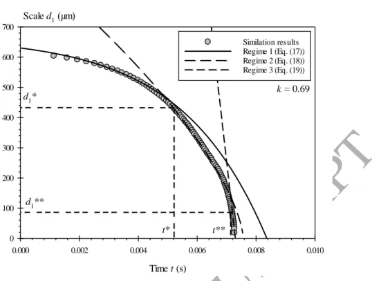
d,t . An example of d1(t) is presented in Fig. 12 (k = 0.69). d1(t)ACCEPTED MANUSCRIPT
22
steps identified in Fig. 4. Furthermore, the dynamics associated to these regimes are those reported in the literature for the neck diameter of the ligament and expressed by Eqs. (8), (10) and (11). The Regime 1 is an exponential decrease similar to the one reported by the linear theory for the neck diameter (see Eq. (8)) and expresses as:
t t exp D d j 8 1 1 (17)
The Regime 2 starts at t = t* for which d1(t*) is noted d1*. The decrease now shows a t2/3
dependence: 3 2 1 1 1 * * * * t t t d d (18)
where the characteristic capillary time t* Ld1*3 . Finally the Regime 3 starts at t = t** for which d1(t**) is noted d1**. The decrease shows a linear dependence with time:
** **** * * t t t d d 1 1 1 (19)
where the characteristic visco-capillary time t** µd1** . The mathematical fits provided by Eqs. (17) to (19) are plotted in Fig. 12. The characteristic times t*, t** and scales d1* and d1** are graphically determined. The three regimes are found for every wavenumber k and the
mathematical fits are determined for each case. Reported in Table 2, the mathematical parameters appear dependent on the wavenumber. The duration of Regime 1, given by the
ACCEPTED MANUSCRIPT
23
time t*, increases with k and the growth rate increases and then decreases. A maximum is found for k = 0.80. These growth rates shown in Fig. 10 are smaller than those reported by the linear theory, except for k = 0.88 and 0.95 for which good agreements are obtained. These differences are attributable to non-linear effects and, once again, show that these effects are negligible for high k. On the other hand, this result says that a growth rate smaller than the one predicted by the linear theory as found for small k is an early manifestation of non-linear effects. Concerning Regimes 2 and 3, we see that their durations decrease when k increases. Furthermore, the increase of their temporal growth rate combined with the decrease of the characteristic times t* and tµ** reveals a tremendous acceleration of the breakup mechanism when the wavenumber increases.
The ligament thinning mechanism identified in the small-scale region is characterized by the stretching rate introduced in Eq. (7) for the case of a cylindrical ligament. In the present simulation, the shape of ligament is not cylindrical at all times. Therefore, the use of the distribution e2(d,t) to calculate the stretching rate is not appropriate. This rate is determined
with the functions e3'
d,t and e3'
d,t which are both independent of d (see Fig. 11). Theaverages in the scale space of e3'
d,t and e3'
d,t are calculated for d < d1. The resultingfunctions are noted e '3
t and e '3
t respectively and:
t e t e t ' ' 3 3 (20)For all wavenumbers, Fig. 13 presents the stretching rate
t as a function of the non-dimensional time t/t*. It appears that
t always increases with time. The thinning mechanism is the small-scale region never stops. In Regime 1 (t/t* < 1), the acceleration of
tACCEPTED MANUSCRIPT
24
a sharp increase of
t . As far as the influence of the wavenumber is concerned, we see that
t increases with k (this behavior is not observed for k = 0.95 in Regime 1 but the acceleration of
t in this regime in higher than for the other wavenumbers). The impact of the continuous thinning mechanism on the specific-surface-area of the whole system can be seen in Fig. 14. This figure presents the temporal evolution of the ligament specific-surface-area e3(0,t) as a function of t/t* for five wavenumbers. The specific-surface-area firstincreases, reaches a maximum and then decreases to a final value smaller than the initial one. This latter point is a characteristic feature of the capillary instability as discussed in Fig. 8. Figure 14 also shows that globally speaking, the increase of the specific-surface-area corresponds to Regime 1 (t/t* < 1). Furthermore the maximum specific-surface-area correlates with the value of the stretching rate. Therefore, the thinning mechanism during Regime 1 produced interface and is likely an elongation mechanism. This is not the case for Regimes 2 and 3 during which the specific-surface-area decreases. In these regimes, the mechanism operating at small scales is likely a contraction mechanism. Note that the dynamics in Regimes 2 and 3 (Eqs. (18) and (19)) are known in the literature to be associated to capillary contraction mechanisms. To confirm these conclusions the volume of liquid subject to the thinning mechanism in the small scales should be evaluated during time. This is the purpose of the simple model presented in the last section.
4.3 Model of the scale distribution e3(d,t)
If we consider a System 1 with a volume-based scale distribution e3,1(d,t) and a System 2 with
a scale distribution e3,2(d,t), the scale distribution of the system made by the sum of Systems 1
and 2 is the sum of e3,1(d,t) and e3,2(d,t) each of them being weighted by the relative volume
they represent. The idea of the present model is to apply such a decomposition to the scale distribution of the liquid ligament at each time, i.e.:
ACCEPTED MANUSCRIPT
25
d t t e d t
t
e d te3 , 3,1 , 1 3,2 , (21)
where (t) indicates the relative volume of System 1: (t) = V1(t)/VT where V1(t) is the
volume of System 1, V2(t) is the volume of System 2 and VT is the total system volume
(VT = V1(t) + V2(t)). The decomposition expressed by Eq. (21) is built so that System 1 is
subject to the thinning mechanism identified at small scales and System 2 is subject to the thickening mechanism identified in the large scales. At small scales, the thinning mechanism is similar to the thinning of a cylindrical ligament. System 1 is therefore chosen as a cylindrical ligament with a diameter D1(t), i.e. (see Eq. (5)):
t D d t D t d e 1 1 1 , 3 1 2 , (22)Being subject to the thickening mechanism, System 2 must evolve from a cylinder to a sphere. According to Eq. (5), the volume-based scale distribution of such a system can be written:
1 2 2 2 , 3 , 1 t n t D d t D t n t d e (23)where n(t) varies from 2 to 3. At initial time, System 2 is a cylinder and n(t) = 2 and D2(t) is
the diameter of the cylinder. At final times, System 2 approaches a sphere and n(t) approaches 3 and D2(t) is the diameter of this sphere. The combination of Eqs. (21-23) leads to:
ACCEPTED MANUSCRIPT
26
d t D t d e t D d t D t D d t D t n t t d e t D d t D d t D t n t t D d t D t t d e t n t n 2 3 2 1 1 2 2 3 1 1 2 2 1 1 3 for 0 , for 1 1 , 0 for 1 1 1 2 , (24)To complete the model, the functions D1(t), D2(t), (t) and n(t) must be determined. The
diameter D2(t) is also the maximum scale dmax(t). We therefore impose:
t d
tD2 max (25)
The thinning mechanism in the small-scale region introduces two characteristic scales: the one used in the calculation of the stretching rate, i.e. 2 e '3
t (see Eq. (20)) and the one delimiting the small-scale region, i.e., d1(t). The diameter D1(t) should include these twoscales. We suggest:
2 , 0 ' 2 3 1 1 t e t d t D (26)The functions (t) and n(t) are then determined by using e3(0,t) and e3'
0,t . Equation (24)allows writing the following system:
2 2 2 1 3 2 1 3 1 1 2 , 0 ' 1 2 , 0 t D t n t n t t D t t e t D t n t t D t t e (27)ACCEPTED MANUSCRIPT
27
The system of Eq. (27) is solved using Eqs.(25) and (26). Scales dmax and d1 that appear in
Eqs. (25) and (26) are calculated from Eq. (16) and Eqs. (17) to (19), respectively. (The parameters for each equation are given in Tables 1 and 2.) Furthermore, the measured values for e3(0,t) and e3'
0,t are used in Eq. (27). During the resolution of Eq. (27), we pay attentionto maintain n(t) between 2 and 3. If n(t) < 2 (which can happen at early times) we impose n(t) = 2 and if n(t) > 3 (which can happen at later times) we impose n(t) = 3. In both cases, the corresponding (t) is determined from the first equation of Eq. (27). Finally, if the condition n(t) = 3 returns a negative (t), then the condition (t) = 0 is imposed and n(t) is determined accordingly. In every case, the application of this model gives satisfactory results. Two examples are shown in Fig. 15 (k = 0.55). At t = 7.71 ms, we see that the slope change between the small-scale and the large-scale regions is found by the model at a higher scale. This problem is believed to be related to the approximation chosen for the parameter D1(t)
(Eq. (26)). The disagreement caused by this choice is never greater than the one shown in Fig. 15.
Figure 16 presents the specific-surface-area of System 1 as a function of t/t* for five wavenumbers. Since System 1 is subject to a thinning mechanism, its specific-surface-area always increases with time. In Regime 1, this increase is independent of the wavenumber. In Regimes 2 and 3, the increase rate of e3,1(0,t) increases with the wavenumber. Similarly, Fig.
17 presents the specific-surface-area of System 2 as a function of t/t* for five wavenumbers and Fig. 18 shows the corresponding evolution of the parameter n(t). During the first period of time, e3,2(0,t) decreases with time while the parameter n(t) is constant and equal to 2. Thus,
System 2 is a thickening cylinder during this period. Then, e3,2(0,t) increases with time while n(t) increases. The increase of n(t) illustrates a deformation of System 2 and explains the
ACCEPTED MANUSCRIPT
28
increase in specific-surface-area. Finally, when n(t) has reached its final value, e3,2(0,t)
decreases again. Note that the final value of n(t) is less than 3 for the high wavenumbers since the swollen part of the ligament is not spherical as noticed in Fig. 5.
Finally, the parameter (t) is shown in Fig. 19 for the same k as in Figs. 16 to 18. Globally speaking, (t) is almost constant during Regime 1 (t/t* < 1) meaning that the volumes of Systems 1 and 2 are almost constant. System 1 is therefore a cylinder with an increasing specific-surface-area and a constant volume: it is subjected to an elongation mechanism. During Regime 1, an elongation mechanism controls the small scale dynamics in the capillary instability. Note that whereas the specific-surface-area evolution is not a function of the wavenumber (Fig. 16), the proportion of liquid concerned by this mechanism increases with k. Indeed, Fig. 19 reports an increase of (t) with the wavenumber. However, since the total volume of the ligament decreases as k increases (VT = 2Dj3/k), the initial volume of System 1
(at t = 0) always decreases with k.
For t/t* > 1, (t) decreases with time. System 1 is subjected to a mechanism that increases its specific-surface-area (Fig. 16) and decreases its volume. This confirms that the mechanism in Regimes 2 and 3 is a contraction mechanism due to surface tension forces. In Regime 2, the contraction mechanism is therefore controlled by inertia forces whereas it is controlled by viscous forces in Regime 3. Figure 19 also shows that (t) is fairly independent of k at t/t* = 1. Therefore the volume of System 1 at the beginning of Regime 2 decreases with k. This explains why the duration of the capillary driven contraction mechanisms in Regimes 2 and 3 significantly decreases as the perturbation wavenumber k increases.
The capillary instability of a cylindrical ligament is a process where the mechanism of breakup is always preceded by an elongation mechanism at small scales. When k increases, this elongation mechanism reaches higher stretching rates and it is found that the subsequent contraction mechanism is delayed and the pinch-off occurs on smaller threads, creating
ACCEPTED MANUSCRIPT
29
smaller satellite drops. Furthermore, all this is accompanied by a smaller reduction of the specific-surface-area of the system. We therefore see that an elongation mechanism at small scale is favorable to a better atomization. This conclusion agree with the one reported by Marmottant and Villermaux (2004) on the behavior of stretched liquid ligaments.
ACCEPTED MANUSCRIPT
30
5 Conclusion
The multi-scale analysis of the simulated capillary instability of cylindrical liquid ligaments relies on the measurement of the scale distribution en(d,t). Using images of the 2D projection
of the ligament, the surface-based scale distribution e2(d,t) is obtained. Furthermore, since the
ligaments are axisymmetric, the volume-based scale distribution e3(d,t) is obtained also. At d = 0, this latter distribution reports the specific-surface-area of the ligament which is a characteristic feature in liquid atomization processes.
During the capillary instability, the scale space may be divided in two regions, i.e., the small-scale region where a thinning mechanism operates and the large-small-scale region where a thickening mechanism is identified. The regions are respectively associated with the characteristic scales d1(t) and dmax(t). These two characteristic scales report different
dynamics. The dynamic of dmax(t) fully agrees with the one reported by the linear theory
which is not the case for d1(t). This result says that the non-linear effects mainly affect the
small-scale dynamics. In agreement with works of the literature, it is found that these effects are less pronounced as the wavenumber increases.
The dynamics of the characteristic scale d1(t) follows three successive regimes.
Mathematically speaking, Regime 1 reports an exponential dependence with time similar to the linear theory prediction. It is found that the growth rate is less than the one reported by the theory when non-linear effects are non-negligible. During Regimes 2 and 3, d1(t) shows a
temporal dependence as t2/3 and t, successively, corresponding to the dynamics of the pinch-off mechanism reported in the literature. The presence of these regimes indicate that the small scales are subjected to successive mechanisms. Thanks to a simple model, these mechanisms have been identified. Regime 1 corresponds to an elongation mechanism which results in the increase of the specific-surface-area of the ligament. Regimes 2 and 3 correspond to a contraction mechanism due to surface tension forces and successively controlled by inertia
ACCEPTED MANUSCRIPT
31
and viscous forces. These regimes contribute to a decreases of the specific-surface-area of the ligament.
When k increases, the duration and stretching rate of the elongation mechanism increase. The effect of this is to damp the surface tension contraction and to delay the pinch-off mechanism. The live time of the elongation mechanism is therefore very important. We believe it to be directly connected with the temporal evolution of the shape of the swollen part of the ligament which also strongly depends with k. Further investigation should be performed on this point. This work shows to which extend the multi-scale analysis used here can help identifying and characterizing the basic mechanisms involved in the evolution of a two-phase system whose interface area continuously varies with time. It must be borne in mind that the present conclusions are valuable for the working conditions of this study only and, in particular, for a given initial amplitude of the perturbation. It is known that this parameter influences the non-linear effects in capillary instability of liquid ligaments. The influence of this parameter on the present conclusions would be indeed an interesting and valuable complement to this work.
Acknowledgments
The authors acknowledge the financial support from the French National Research Agency (ANR) through the program Investissements d’Avenir (ANR-10 LABX-09-01), LABEX EMC3. All simulations have used the facilities of CRIANN (Centre Régional Informatique et d’Applications Numériques de Normandie).
ACCEPTED MANUSCRIPT
32
REFERENCES
Aniszewski, W., Ménard, T., Marek., M. 2014 Volume of fluid (vof) type advection methods in two-phase flow: A comparative study. Computers & Fluids, 97, 52-73
Amarouchene, Y., Bonn, D., Meunier, J., Kelay, H. 2001 Inhibition of the finite-time singularity during droplet fission of a polymeric fluid. Physical Review Letters 16, 3558-3561 Ashgriz, N., Mashayek, F. 1995 Temporal analysis of capillary jet breakup. Journal of Fluid Mechanics 291, 163-190
Ashgriz, N., Yarin, A.L. 2011 Handbook of Atomization and Sprays: Chapter 1-Capillary of free liquid jets (ed. N. Ashgriz,) pp. 3-53, Springer Science+Business Media
Berlemont, A., Blaisot, J.B., Bouali, Z., Cousin, J., Desjonqueres, P., Doring, M., Dumouchel, C., Idlahcen, S., Leboucher, N., Lounacci, K., Ménard, T., Rozé, C., Sedarsky, D., Vaudor, G. 2013 Numerical simulation of primary atomization: Interaction with experimental analysis. Atomization and Sprays, 23, 1103-1138
Bérubé, J., Jébrak, M. 1999 High precision boundary fractal analysis for shape characterization. Computers & Geosciences 25, 1059–1071.
Bogy, D.B. 1979 Drop formation in a circular liquid jet. Annual Review of Fluid Mechanics
11, 207-228
Brandt, A. 1984 Multigrid Techniques: 1984 guide with applications to fluid dynamics. GMD-Studien
Brenner, M.P., Eggers, J., Joseph, K., Nagel, S.R., Shi, X.D. 1997 Breakdown of scaling in droplet fission at high Reynolds number. Physics of Fluids 9, 15731590
Dumouchel, C. 2008 On the experimental investigation on primary atomization of liquid streams. Experiments in Fluids 45: 371-422
ACCEPTED MANUSCRIPT
33
Dumouchel, C., Blaisot, J.B., Bouche, E., Ménard, T., Vu, T.T. 2015a Multi-scale analysis of atomizing liquid ligaments. International Journal of Multiphase Flow 73, 251-263
Dumouchel, C., Grout, S. 2009 Application of the scale entropy diffusion model to describe a liquid atomization process. International Journal of Multiphase Flow 35, 952-962
Dumouchel, C., Grout, S. 2011 On the scale diffusivity of a 2-D liquid atomization process analysis. Physica A 390, 1811-1825
Dumouchel, C., Ménard, T., Aniszewski, W. 2015b Towards an interpretation of the scale diffusivity in liquid atomization process: An experimental approach. Physica A 438, 612-624 Duret, B., Luret, G., Reveillon, J., Ménard, T., Berlemont, A., Demoulin, F.X. 2012 DNS analysis of turbulent mixing in two-phase flows. International Journal of Multiphase Flow
40, 93-105
Eggers, J. 1993 Universal pinching of 3D axisymmetric free-surface flow. Physical Review Letters 21, 3458-3460
Eggers, J. 1997 Non-linear dynamics and breakup of free surface flows. Reviews of Modern Physics 69, 865-929
Eggers, J., Dupont, T. 1994 Drop formation in a one-dimensional approximation of the Navier-Stokes equation. Journal of Fluid Mechanics 262, 205-221
Eggers, J., Villermaux, E. 2008 Physics of liquid jets. Reports on Progress in Physics 71, 036601 1-79
Evers, L.W. 1994 Analogy between atomization and vaporization based on the conservation of energy. SAE Technical Series, Paper n°940190.
Fedkiw, R., Aslam, T., Merriman, B., Osher, S. 1999 A non-oscillatory eulerian approach to interfaces in multimaterial flows (the ghost fluid method). Journal of Computational Physics, 152, 457-492
ACCEPTED MANUSCRIPT
34
Goedde, E.F., Yuen, M.C. 1970 Experiments on liquid jet instability. Journal of Fluid Mechanics 40, 495-511
Kang, M., Liu, X., Fedkiw, R. 2000 Boundary condition capturing method for multiphase incompressible flows. Journal of Scientific Computing 15, 323-360
Kowalewski, T.A. 1996 On the separation of droplets from a liquid jet. Fluid Dynamics Research 17, 121-145
Lister, J.R., Stone, H.A. 1998 Capillary breakup of a viscous threads surrounded by another viscous fluid. Physics of Fluids 10, 2758-2764
Marmottant, P., Villermaux, E. 2004 Fragmentation of stretched liquid ligaments. Physics of Fluids 18(8), 2732-2741
Ménard, T., Tanguy, S., Berlemont, A. 2007 Coupling level set/ volume of fluid/ ghost fluid methods, validation and application to 3d simulation of the primary breakup of a liquid jet. International Journal of Multiphase Flow 33, 510-524
Osher, S., Fedkiw, R. 2001 Level set methods: An overview and some recent results. Journal of Computational Physics 169, 463-502
Osher, S., Sethian, J. 1988 Fronts propagating with curvature dependent speed: Algorithms based on hamilton-jacobi formulation. Journal of Computational Physics 79, 12-49
Papageorgiou, D.T. 1995 On the breakup of viscous liquid threads. Physics of Fluids 7, 1529-1544
Pimbley, W.T. Lee, H.C. 1977 Satellite droplet formation in a liquid jet. IBM Journal of Research and Development 21, 21-31
Plateau, J., 1849, Statique Expérimentale et Théorique des Liquides Soumis aux Seules Forces Moleculaires. Académie des Sciences de Bruxelles Mémoire 23, 5
Rayleigh, Lord, J.W.S. 1878 On the instability of jets. Proceedings of the London Mathematical Society 10, 4-13
ACCEPTED MANUSCRIPT
35
Rutland, D.F., Jameson, G.J. 1971 A non-linear effect in the capillary instability of liquid jets. Journal of Fluid Mechanics 46, 267-271
Shu, C.W. 1997 Essentially Non-Oscillatory and Weighted Essentially Non-Oscillatory Schemes for Hyperbolic Conservation Laws. NASA (as report NASA/CR-97-206253)
Stelter, M., Brenn, G., Yarin, A.L., Singh, R.P., Durst, F. 2000 Validation and application of a novel elongation device for polymer solutions. Journal of Rheology 44, 595-616
Sussman, M., Puckett, E.G. 2000 A coupled level set and volume-of-fluid method for computing 3d axisymmetric incompressible two-phase flows. Journal of Computational Physics 162, 301-337
Tanguy, S., Berlemont, A. 2005 Application of a level set method for simulation of droplet collisions. International Journal of Multiphase Flow 31, 1015-1035
Tryggvason, G., Scardovelli, R., Zaleski, S. 2011 Direct Numerical Simulations of Gas-Liquid Multiphase Flows. Cambridge Monographs
Vassallo, P., Ashgriz, N. 1991 Satellite formation and merging in liquid jet breakup. Proceeding of the Royal Society of London A. 433, 269-286
Yuen, M.C. 1968 Non-linear capillary instability of a liquid jet. Journal of Fluid Mechanics
ACCEPTED MANUSCRIPT
36
Fig. 1. Temporal evolution of an atomizing water ligament into air. Time gap between two consecutive images 40 µs. IC: Local specific-interface-area creation; IR: Local specific-interface-area reduction (From Dumouchel et al.; 2015a)
Fig. 2. Illustration of an erosion operation. Left: Initial 2-D system. Its total surface area is noted S2T; Right: Erosion at scale d. The light gray strip is removed. The eroded
ACCEPTED MANUSCRIPT
37 Scale d (AU) e2(d,t) (AU-1) t1 t2 t3 t4 D(t1) D(t2) D(t3) D(t4) 1/D(t1) 1/D(t2) 1/D(t3) 1/D(t4) t1 < t2 < t3 < t4 0 0 t = 5.50 ms t = 0 ms t = 2.30 ms t = 6.50 ms t = 4.60 ms t = 7.96 ms t = 8.05 ms t = 8.13 ms t = 7.50 msACCEPTED MANUSCRIPT
38 Scale d (AU) e3(d,t) (AU-1) t1 t2 t3 t4 D(t1) D(t2) D(t3) D(t4) 2/D(t1) 2/D(t2) 2/D(t3) 2/D(t4) t1 < t2 < t3 < t4 0 0Fig. 3. Temporal evolution of the scale distribution of a thinning cylindrical ligament: a – e2(d,t), b – e3(d,t)
Fig. 4. Simulation results. Temporal evolution of the ligament for k = 0.55
t = 5.50 ms t = 0 ms t = 2.30 ms t = 6.50 ms t = 4.60 ms t = 7.96 ms t = 8.05 ms t = 8.13 ms t = 7.50 ms
ACCEPTED MANUSCRIPT
39 Scale d (µm) 0 200 400 600 800 1000 1200 1400 1600 e2(d,t) (µm -1 ) 0.0000 0.0005 0.0010 0.0015 0.0020 0.0025 0 ms 5 ms 6.5 ms 7.5 ms 8 ms 8.13 ms k = 0.55 Scale d (µm) 0 200 400 600 800 1000 1200 e3(d,t) (µm -1 ) 0.0000 0.0005 0.0010 0.0015 0.0020 0.0025 0.0030 0.0035 0 ms 5 ms 6.5 ms 7.5 ms 8 ms 8.13 ms k = 0.55Fig. 5. Simulation results – Shape of the ligament at breakup time, influence of the wavenumber (The images are on scale with each other, their width represents /2. The number in parenthesis is the ratio tBU/tBUtheo)
ACCEPTED MANUSCRIPT
40 time t (s) 0.000 0.002 0.004 0.006 0.008 0.010 d3 (µm) 600 700 800 900 1000 1100 1200 1300 k = 0.55 k = 0.69 k = 0.88 k = 0.95 k = 0.55 Math. Beh. k = 0.69 Math. Beh. k = 0.88 Math. Beh. k = 0.95 Math. Beh. Scale d (µm) 0 200 400 600 800 1000 1200 1400 1600 e2(d,t) (µm-1) 0.0000 0.0005 0.0010 0.0015 0.0020 0.0025 0 ms 5 ms 6.5 ms 7.5 ms 8 ms 8.13 ms k = 0.55ACCEPTED MANUSCRIPT
41 Scale d (µm) 0 200 400 600 800 1000 1200 e3(d,t) (µm-1) 0.0000 0.0005 0.0010 0.0015 0.0020 0.0025 0.0030 0.0035 0 ms 5 ms 6.5 ms 7.5 ms 8 ms 8.13 ms k = 0.55Fig. 6. Temporal evolution of the scale distributions for k = 0.55: a – e2(d,t), b – e3(d,t)
Scale d (µm) 0 200 400 600 800 1000 1200 1400 e2(d,tBU) (1/µm) 0.0000 0.0005 0.0010 0.0015 0.0020 0.0025 k = 0.55 k = 0.69 k = 0.80 k = 0.88 k = 0.95
ACCEPTED MANUSCRIPT
42 k (-) 0.3 0.4 0.5 0.6 0.7 0.8 0.9 1.0 1.1 e3(0,t) (1/µm) 0.0025 0.0026 0.0027 0.0028 0.0029 0.0030 0.0031 t = 0 t = tBUInitial unperturbed system Linear theory
Dj = 666 µm
Fig. 8. Initial and Final specific-surface-area as a function of the wavenumber k. Comparison between the simulation results and the linear theory
time t (s) 0.000 0.002 0.004 0.006 0.008 0.010 dm ax (µm) 600 700 800 900 1000 1100 1200 1300 k = 0.55 k = 0.69 k = 0.88 k = 0.95 k = 0.55 (Eq. (16)) k = 0.69 (Eq. (16)). k = 0.88 (Eq. (16)) k = 0.95 (Eq. (16))
Fig. 9. Temporal evolution of the scale dmax for several wavenumbers and mathematical fit