Continuous production of conducting polymer

MITLibraries

http: //libraries. mit. edu/docs

DISCLAIMER OF QUALITY

Due to the condition of the original material, there are unavoidable

flaws in this reproduction. We have made every effort

possible

to

provide you with the best copy available. If you are dissatisfied with

this product and find it unusable, please contact Document Services as

soon

as possible.

Thank you.

Some pages in the original document contain color

Continuous Production of Conducting Polymer

by Terry A. Gaige

Submitted to the Department of Mechanical Engineering in Partial Fulfillment of the Requirements for the Degree of

Bachelor of Science in Mechanical Engineering

at the

Massachusetts Institute of Technology

June 2004

©2004 Terry A. Gaige. All rights reserved.

The author hereby grants to MIT permission to reproduce and to distribute publicly paper and electronic copies of this thesis document in whole or in part.

MASSACHUSETTS INSTIUTE OF TECHNOLOGY OCT 2 8 2004

LIBRARIES

DepaAment of l(lchanical Engineering May 6, 2004

Certified by:

Hastopoulos Professor of Mechanical

Accepted by:

Ian W. Hunter Engineering and Professor of BioEngineering Thesis S4pervisor

Ernest G. Cravalho Professor of Mechanical Engineering Chairman, Undergraduate Thesis Committee

ARCHIVES

1

i i

Continuous Production of Conducting Polymer

by Terry A. Gaige

Submitted to the Department of Mechanical Engineering on May 7, 2004 in Partial Fulfillment of the Requirements for the Degree of Bachelor of

Science in Mechanical Engineering

Abstract

A device to continuously produce polypyrrole was designed, manufactured, and tested. Polypyrrole is a conducting polymer which has potential artificial muscle applications. The objective of continuous production was to produce both larger films and films with more consistent properties than the films produced by the current batch-production method. The mechanical properties of polymers produced by batch synthesis are known to be highly dependent on reaction parameters such as temperature, and reactant and electrolyte concentrations. A system of peltier thermoelectric coolers and refrigerated-circulator held the deposition chamber at -10 °C. The polypyrrole film deposited onto the surface of a rotating glassy carbon crucible was peeled off using a blade and spring force

mechanism. The temperature, current, and voltage of the electrodeposition were

recorded. Several successful, but short, continuous deposition trials were run at a current

density of 0.5 A/m2and a film 50 mm long and 0.246 mm thick was produced and tested.

High rate depositions were also attempted at 150 A/m2 but failed due to over-oxidation.

In this thesis, it is demonstrated that continuous production appears feasible. A second prototype of the device is proposed with several improvements, the most important of which are a larger torque applied to the rotating crucible and a more effective and efficient cooling mechanism.

Thesis Supervisor: Ian W. Hunter

Table of Contents

List of Figures and Tables 7

Acknowledgements 9

1.0 Introduction and Background 11

2.0 Previous Methods and Limitations 12

2.1 Characteristics of batch-produced polypyrrole 12

2.2 Previous attempts at continuous production 13

2.2.1 Outside of MIT Biolnstrumentation Lab 13

2.2.2 Within the MIT Biolnstrumentation Lab 13

3.0 Theory, Design and Manufacture of First Prototype 13

3.1 Cooling of Deposition Chamber 15

3.1.1 Peltier Thermoelectric Coolers 15

3.1.2 Serpentine Channel Heat Dissipater 21

3.1.3 Refrigerated-circulator 22

3.2 Crucible and Counter-Electrode 23

3.2.1 Rotating 23

3.2.2 Peeling 24

3.3 Deposition Control Center Instrumentation and Software 27

3.3.1 Measurements 27

3.3.2 Controls 28

3.3.3 Actuators 28

4.0 Experimental Procedure 29

4.1 System Characterizations 29

4.1.1 Peltier/Refrigerated-Circulator System Test 29

4.1.2 Stepper Motor Test 32

4.1.4 Rate of Deposition 34

4.2 Experimental Results 36

4.2.1 Apparatus 36

4.2.1 Methods 37

5.0 Results and Discussion 40

5.1 Typical Deposition 40

5.2 High Rate Deposition 44

6.0 Conclusion 46

7.0 Future Work 46

References 49

Appendix A- Polypyrrole Batch-deposition Method 51

Appendix B - Peltier specifications 53

Appendix C - Corrosion Resistance of Plastics to Propylene Carbonate Solution 54

List of Figures and Tables

Figure 1: Completed schematic for the continuous production of polypyrrole. 14

Figure 2: Diagram of deposition chamber. 15

Figure 3: Diagram of a peltier thermoelectric cooler. 16

Figure 4: Diagram of the passive heat load due to conductive and convective heat transfer

to the solution from the environment. 16

Figure 5: Characteristic curves for the HP- 199-1.4-1.15 peltier - temperature difference

vs. current. 19

Figure 6: Characteristic curve for the HP-199-1.4-1.15 peltier - voltage vs. current _ 20

Figure 7: CAD model showing the design of the serpentine channel heat dissipater on the

bottom and sides of the cooling chamber. 22

Figure 8: CAD Model of the crucible support which was printed on a Viper stereo

lithography machine. 23

Figure 9: Photo of crucible, stepper motor, and peeling mechanism. 24

Figure 10: Force diagram of peeling mechanism. 25

Figure 11: Plot of minimum required motor torque for varying peeling blade angle and

coefficient of friction. 26

Figure 12: Screen shot of graphic user interface for the Visual Basic .NET program used

to control and record parameters during a deposition. 27

Figure 13: Diagram of the locations of recorded temperatures (T) within deposition

chamber. 30

Figure 14: Plot showing temperatures at the four locations when 6V, 7V, 8V and 9V were

applied to the twelve peltier TECs in parallel. 31

Figure 15: Mechanisms of polypyrrole polymerization. 33

Figure 16: Plot of amount of molecules that would be deposited on surface of crucible

with all assumptions for a high current deposition. 35

Figure 17: Plot of concentrations of reactants as time passes with all the assumptions for

a high current deposition 35

Figure 18: The completed cooling chamber and peeling mechanism. 36

Figure 19: Photo of entire experimental set-up which includes three power supplies, a chiller/circulator, a data-acquisition unit connected to a standard PC, and the

deposition chamber within the insulating box. 37

Figure 20: Photo of cooling deposition chamber containing solution and with copper

counter-electrode installed. 38

Figure 21: Typical plot of recorded values of solution temperature and the electrode

voltage and current for a full continuous deposition trial. 40

Figure 22: Photo of deposition during which the stepper motor failed to turn. The film on the bottom half of the crucible bubbled and began to separate from the surface. _ 42 Figure 23: Photo of a successful deposition. The blade has started peeling the

polypyrrole off of the crucible. 43

Figure 24: Photo of a piece of produced polypyrrole. 43

Figure 25: Screenshot of the stress-strain results of DMA test of 2 mm wide sample of

polypyrrole. 44

Acknowledgements

I would like to thank Patrick Anquetil for his knowledge, support, and continuous guidance. I would also like to thank my co-student-researchers on this project: Brian Keegan for his amazing solid modeling skills and Nikhil Shenoy for his inate programming ability. And, of course, I would like to express grateful appreciation to Professor an Hunter for the opportunity to work with him and his colleagues in the

1.0 Introduction and Background

Polymers are long molecules composed of repeated subunits. There are natural polymers such as DNA, proteins and cellulose and many synthetic polymers such as plastics. Polymers are generally considered insulators and are widely used for that property; however, scientists discovered a class of polymers that has a high electrical conductivity due to its specific molecular structure. In order for a polymer to conduct electricity, the electrons need to be free to move. In a conducting polymer, the electrons can flow down a backbone of alternating single and double bonds, called conjugated double bonds. Another requirement before the electrons are free to move is a disturbance of the basic material structure by the addition or subtraction of electrons, a process known as doping. Some conducting polymers have unique properties such as photoluminescence and contractibility. The material can be both power-efficient and chemically inert so it could prove very useful for medical applications. Other potential applications of conducting

polymers include batteries, biosensors, antistatic clothing1, photovoltaic devices2,

wine-tasting sensors3, robotic actuators, visual displays and more.

Polypyrrole is one of several different conducting polymers whose properties are being studied and practical applications as engineering materials being explored. Currently, the Conducting Polymer Group in the Biolnstrumentation Laboratory at the Massachusetts Institute of Technology (MIT BiLab) has been optimizing current technology by finding ways to maximize the stress and strain capabilities of polypyrrole and improve strain rate,

efficiency and conductivity. MIT BiLab has also been experimenting with novel

molecular designs and new manufacturing techniques. The subject of this thesis is the development of a method to continuously produce polypyrrole.

Two common methods to produce polypyrrole are by galvanostatic (constant current) or potentiostatic (constant voltage) deposition onto a surface. In a solution containing pyrrole monomer, a small current is run from a copper cathode to a glassy carbon

1 Yamato, H., Kai, K., Ohwa, M., Asakura, T., Koshiba, T., Wernet, W., Sythetic Metals 83 (1996) 125-130.

2Lu, S.L., Yang, M.J., Luo, J., Cao, Y., Sythnthetic Metals 140 (2-3): 199-202 FEB 27 2004 3 Riul, A., de Sousa, H.C., Malmegrim, R.R., dos Santos, D.S., Carvalho, A.C.P.L.F., Fonseca, F.J., Oliveira, O.N., Mattoso, L.H.C. Sensors and Actuators B-Chemical 98 (1): 77-82 MAR 1 2004

crucible anode. After about 24 hours (depending on the current), a thin film will have been deposited on the surface of the crucible. This film is then delicately peeled off by hand using a razor blade. The electrical and mechanical properties of the polymers synthesized by this method are dependent on the precise concentrations of reactants, the pH of the solution, and the temperature of the solution. As a deposition progresses, the monomer concentration decreases and pH changes which result in films with varying characteristics throughout.

In this research project, a machine to continuously produce polypyrrole was designed, built, and tested. The advantage of continuously producing conducting polymer is not only to have larger pieces, but also to better monitor its production and get greater consistency, repeatability, and quality. The pH, temperature and monomer concentration had to be continually monitored and controlled and the polymer had to be automatically peeled, treated, and stored as it was produced. Chapter 2 covers previous production methods and also previous attempts at continuous production, none of which succeeded in becoming viable options for continuous production commercially or in a lab. In Chapter 3, the design and theoretical analysis of the first prototype are explained. Chapter 4 describes the system characterizations and trials performed. The final Chapter 5 comments on the partly successful results and makes suggestions for a second prototype.

2.0 Previous Methods and Limitations

The MIT BiLab has been researching the properties of polypyrrole since the early 90's. Several methods of production have been explored but the main method is a batch

production.4

2.1 Characteristics of batch-produced polypyrrole

Polypyrolle films are grown in a propylene carbonate solution with 0.05 M pyrrole monomer, 0.05 M tetraethylammonium hexaflourophosphate (TEAP) and 1% vol. distilled water. The method is described in detail in Appendix A. The solution is poured into a large beaker containing a glassy carbon crucible surrounded by a copper sheet,

4 Madden, J., Conducting Polymer Actuators, Ph.D. Thesis, Massachusetts Institute of Technology, Cambridge, MA, September 2000; p. 34.

which serves as the counter electrode. The electrodepositions are run at -40 C with galvanostatic control. During the deposition, measurements of temperature, current and voltage are taken, but no control is implemented. Depositions are typically run at a 1.25

A/m2 for 16 hours and produce films 28 Am thick. Films have been produced up to 2 m

in length using a spiral coil geometry on the crucible. The maximum active stress tested

was 40 MPa and the greatest active strain was 2%. The highest conductivity to date is 5x 104 S/m.

2.2 Previous attempts at continuous production

The continuous production of conducting polymers has been attempted by many groups. Most often the method of a rotating cyclindrical working electrode was implemented. Groups, such as the International Research Laboratories in Japan and the Intelligent Polymer Research Laboratory in Australia, have succeeded in continuously producing

and peeling a polymer film. The films produced had consistently repeatable

conductivities, but were poor. They reported conductivities on the order of 3.104 S/m and inferior elasticities.

2.2.2 Within the MIT Biolnstrumentation Lab

Several years prior to this research the MIT BiLab realized the potential usefulness of a machine to continuously produce conducting polymer and an attempt was made. The

rotating cylindrical working electrode method was employed. Difficulty was

encountered because the method required large volumes of the solution. Also, no peeling mechanism was used and no temperature control implemented.

3.0 Theory, Design and Manufacture of First Prototype

There are multiple methods to continuously produce a polymer such as solution drawing and fiber deposition. The rotating drum method was chosen for this project because the MIT BiLab has extensive experience with the deposition of polypyrrole onto cylindrical

crucibles. Also, the sheet form produced is useful for bilayer or trimorph actuators5 and

in biomimetic applications such as the fish fin - both subjects being researched over a

5 Schmid, B., Device Design and Mechanical Modeling of Conducting Polymer Actuators, B.S. Thesis, Massachusetts Institute of Technology, Cambridge, MA, June 2003; pp. 23-37.

long period of time in the MIT BiLab. A machine to continuously produce polypyrrole requires continued monitoring and precision control of temperature, pH, reactant concentration, and, in the case of the rotating drum method, a device for peeling and storing the film. Figure 1 shows a schematic for the continuous production method that was employed. A computer receives signals from sensors and sends commands to reactant injection devices, the reaction-driving current generator, the crucible stepping motor, and the peltier thermoelectric heat pumps.

Figure 1: Completed schematic for the continuous production of polypyrrole.

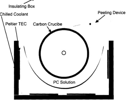
Another possible design was considered in which the propylene carbonate solution would be externally circulated through a chiller, through a mixing/sensing device, then through the deposition chamber; but this design was rejected because it required much larger volumes of the costly chemicals. The design shown in Figure 2 was chosen because the crucial variables such as temperature and reactant concentrations could be readily and precisely controlled within the deposition chamber.

Insulating Box

JeVIL

Figure 2: Diagram of deposition chamber.

3.1 Cooling of Deposition Chamber

In order to maintain the propylene carbonate solution at the required -40 °C, a system with a refrigerated-circulator and peltier thermoelectric coolers (peltiers) was used. This system combined the large cooling power of a refrigerated-circulator with the precise, quick-response controllability of peltiers.

3.1.1 Peltier Thermoelectric Coolers

The selection of peltier thermoelectric coolers is a difficult process because the design equations are either very complex or overly simple to be usefully approximate. Figure 3 shows a diagram of a peltier.

cold side _ semicondi of p-typ se I I - r , I rICl sI (ceramics) "P-ctor :er) hot side

-Figure 3: Diagram of a peltier thermoelectric cooler6.

Heat flows into the cold side from a thermal load and out the hot side into some type of heat sink. The thermal load is a combination of active load and passive load. All loads have a passive component because it is impossible to perfectly thermally isolate anything from conductive, convective and radiative heat. Some sources have an active component, such as computer chips which produce a certain amount of electrical heat or solutions in which an exothermic reaction is taking place. In this project's application, the thermal load is completely passive, meaning that there is no internal heat source and that the thermal load results entirely from the radiation, conduction and convection from the environment as shown in Figure 4.

Tair= 25°C

hwal

hsurf

,all = O°C

vall

Figure 4: Diagram of the passive heat load due to conductive and convective heat transfer to the solution

from the environment.

Ou 70 60 & 50 4 40 I-30 20 10 0 0.0 1.0 2.0 3.0 4.0 5.0 6.0 7.0 8.0 9.0 current (amps) --4-O W -- 12W -- 24W -- 36W -- 48W -4060W --- 71 W- 83W -41-95W -E-107W

Figure 5: Characteristic curves for the HP-199-1.4-1.15 peltier - temperature difference vs. current.8

It is known that Qload is around 33.5 W. Twelve peltiers were used to uniformly

surround the solution, therefore the thermal load on each was 2.8 W. Figure 5 shows

that, for a Ql,ad between 0 W and 12 W and temperature difference of 40 °C, the current

draw by the peltier will be about 2.5 A. Figure 6 is another graph provided by the manufacturers and can be used to estimate the voltage.

8 Taken from http://www.tetech.com/modules/graphs/HP- 199-1.4-1.15.pdf

30 25 20 uR > Z e) 15 0 10 5 0 0.0 1.0 2.0 3.0 4.0 5.0 6.0 7.0 8.0 9.0 current (amps) "'-Qcold = 0 -DT = 9

Figure 6: Characteristic curve for the HP-1 99-1.4-1.15 peltier - voltage vs. current

The upper line in Figure 6 represents the voltage-current relationship for the ideal case of

zero thermal load; the lower line represents the voltage-current relationship for when the

AT is equal to zero. Since the thermal load is small, the upper line should be used. The voltage corresponding to a current draw of 2.5 A is 10 V.

The heat that exits the hot side of a peltier is equal to the sum of the heat pumped out of the load plus the joule heating due to the current running through the peltier,

Qhot Qload + Vpeltier 'Ipeltier, (5)

where Qhot is the total heat exiting the peltier which needs to be removed by a heat sink,

Qioad is the thermal load as calculated by Equation 1, Vpeler is the supplied voltage and Ipeltier is the supplied current. So, using the above estimations for a voltage and current

draw of 10 V and 2.5 A, the twelve peltiers will create 300 W of internal joule heating. The total heat expelled out the hot side of the peltiers, which has to be removed by the

refrigerator/circulator, is 333.5 W; of which, 33.5 W is from the thermal load.

9 Taken from http://www.tetech.com/modules/graphs/HP-199-1.4-1.15.pdf

The total thermal load is equal to the sum of loads due to each mechanism of heat transfer. The heat flow due to radiation can be ignored because it is clearly much smaller than that from conduction and convection. Therefore, the total thermal load is equal to the sum of the conductive and convective heat from all sides:

n

Qload Qi = Qsurf + Qwall

(1)

The contributions from each mechanism of heat transfer can be estimated by using the material properties, temperature differences, and geometries and Equation 1,

Qi = AT' * Ui Ai, (2)

where Oi is the heat flow through some area, AT. is the temperature difference between the two surfaces, Ui is the equivalent overall heat transfer coefficient per area, and A is the area. The equivalent overall heat transfer coefficient for the walls can be written,

Uwaii = kair (3)

L

where Uall is the equivalent overall heat transfer coefficient for the wall, kair is the

conductivity of air, and L is the distance between the inner wall and outer wall. The equivalent overall heat transfer coefficient for the upper surface can be written,

Usurf = hsurf, (4)

where Usurf is the equivalent overall heat transfer coefficient for the upper surface and

hsurf is the convection heat transfer coefficient between propylene carbonate and still air.

hsu was estimated to be less than 25 W/(m2.K) from common values for convection

coefficients of horizontal plates. By entering the values and material properties in Table

1 and steady state temperatures shown in figure 4 into Equations 3 and 4, the total thermal load, Qload is found to be 33.5 W.

Table 1: Values and material properties used to calculate the thermal load.

Area of walls.

Area of upper surface.

Natural convection heat transfer coefficient for air on horizontal plate.

Temperature difference between inner and outer wall. Temperature difference between solution surface and ambient air.

Conduction heat transfer coefficient for air.

Awaii Asurf hsurf ATar air 2 0.056 m2 0.012 m2 25 W/(m2-K) 40 °C 65 °C 0.025 W/(m2K)

The amount of heat flow that a certain manufactured peltier TEC can produce ranges

from less that 0.5 W to over 200 W. This maximum heat flow is called

Qox

when the peltier is driven at maximum current and voltage, Imax and Vmax and when the

temperature difference is zero. ATmax is the temperature difference between the hot and

cold sides of the peltier at which the reverse, conductive heat flow through the peltier is in equilibrium with the pumped heat flow out when the peltier is driven at maximum

current and voltage.. These characteristic values, Qmrx, Imax, Vmax and ATmx, can usually

be found on the specification sheets for a particular peltier.

The peltier specification graphs provided by the manufacturers can be very useful in determining which peltier to use for a particular application. A desired AT can be estimated by assuming that the hot side of the peltier will be held at a constant 0 °C by a liquid refrigerated-circulator and knowing the desired temperature is -40 °C. The TE

Tech7HP-199-1.4-1.15 was chosen because a AT of 40 °C is right in the middle of its

range as Figure 5 shows. (see Appendix B for more peltier specifications)

Value

The twelvepeltier thermoelectric cooler system is capable of cooling a solution down to -40 C, but the system is very inefficient because the peltiers produce an extra 300 W of joule heating. The advantage of the peltier system is the ability for quick response time

and very accurate holding of temperature.

3.1.2 Serpentine Channel Heat Dissipater

The hot sides of the peltiers were kept cool by contact with aluminum plates containing

serpentine channels with coolant flow. Aluminum was chosen because of its

machinability and high thermal conductivity. The coolant, circulated by a refrigerated-circulator, entered into one face of the box, split into three, flowed through the channels, rejoined and exited out the opposite face. A CAD model of the heat dissipater, shown in

Figure 7, was created using Solid Edge V1410. Then, using FeatureCAM 2004 toolpaths

were created that guided a HAAS VF-0E to mill channels, o-ring grooves and screw

holes into the aluminum plates. To connect the channels from one face to the next, coaxial holes were drilled and o-rings installed at the interface. There could have been an uneven flow distribution between the three faces due to the Coanda effect so a large chamber was milled at the coolant entrance and exit. It this way, a pressure pocket was created which caused the coolant to flow through the somewhat restrictive interface holes

at even rates. To cover the channels, 1Omm thick acrylic was cut to fit with a lasercutter

and sealed with Buna-N o-ring cord stock. Then, for the coolant entrance and exit, brass pipe-to-hose, barbed adapters were threaded into the acrylic.

21

Figure 7: CAD model showing the design of the serpentine channel heat dissipater on the bottom and sides

of the cooling chamber.

3.1.3 Refrigerated-circulator

The requirements of the refrigerated-circulator were to pump the coolant through the

serpentine channels and to maintain the coolant at less than 0 °C. It was found that 333.5

W of heat would flow out of the hot sides of the peltiers and into the aluminum plates (See Section 3.1.1 for detail). Therefore, the refrigerated-circulator had to remove that thermal load as well as the additional thermal load from ambient air conducting into the supply lines.

The only refrigerated-circulator available for use was VWR Signature

Heated/Refrigerated Circulator, Model 1166, with a two-speed pump. The

refrigerated-circulator had a 6 L bath and cooling capacity of 200 W at 20 °C and 140 W at 0 °C,

which was far below the 333.5 W thermal load, not to mention inadvertent loss to ambient air through the tubing. See Section 4.1.1 for a characterization of the systems ability to cool the solution. Although the system was not capable of keeping the solution

at -40 °C, it was able to hold a relatively constant -10 °C which was satisfactory enough

to continue with experimentation.

3.2 Crucible and Counter-Electrode

The same type of glassy carbon crucible as was used in batch-production (see Section

2.1) was used for continuous production, a Sigradur 285 mL G-crucible. The bottom

face was cut out using an abrasive watejet machining center to allow for a continuous solid axle. A crucible support as shown in Figure 8 was printed on a Viper stereo lithography machine. Parts produced in the stereo lithography machine were very useful because the hardened resin was completely resistant to the propylene carbonate solution, unlike many other plastics (see Appendix C for a table of several plastics' resistance to propylene carbonate). The crucible support was given a slight taper to fit with crucibles that did not have perfectly circular cross-sections. A stainless steel axle mounted with two ABEC 5 bearings allowed the crucible to spin freely. A 0.4 mm thick copper sheet 100 mm by 200 mm was used as a counter-electrode. It could be flattened when cleaned and then recurved to match the crucible curvature with approximately a 10 mm separation distance.

Figure 8: CAD Model of the crucible support which was printed on a Viper stereo lithography machine.

3.2.1 Rotating

To get the desired quality of polypyrrole and 25 /zm thickness, a typical batch-deposition was carried out over 16 hours with a 10 mA reaction-driving current. For the equivalent continuous-deposition, where only half the crucible is submerged in solution at any particular time, the crucible must rotate at approximately one revolution every 32 hours to get the same film thickness. The analysis in Section 3.2.2 shows that the crucible must be rotated with at least 0.8 Nm of torque. A stepper motor can meet such requirements for extremely slow speeds and moderate torque. The Zeta 57-83M stepper motor was

Purchased from - Hochtemperatur-Werkstoffe GmbH, Gemeindewald 41, D-86672 Thierhaupten

used in conjunction with a Parker Compumotor 6104 indexer drive. The stepper motor had 0.8 Nm maximum holding torque and was capable of 50,000 microsteps per revolution which allowed for very smooth control at slow speeds. A 70 mm pitch circle diameter aluminum gear with 128 teeth was mounted to the face of the crucible support so that it could be driven by the stepper motor.

3.2.2 Peeling

It was possible to peel the polypyrrole film off of the glassy carbon crucible by hand using a razor blade. With the acquirement of a small amount of technique, the razor blade could be slightly rocked back and forth and the film would come away from the surface intact. Because of the difficulty of mechanizing the rocking technique, it was hypothesized that the same results could be obtained by applying a larger inward radial force with the blade. The device shown in Figure 9 was designed to hold a razor against the surface of the crucible as it was turned by the stepper motor. The blade angle was

adjustable between about 20 and 30 from the tangent to the crucible surface. The

inward radial force could be adjusted by replacing the springs with springs of a different spring constant.

Figure 9: Photo of crucible, stepper motor, and peeling mechanism.

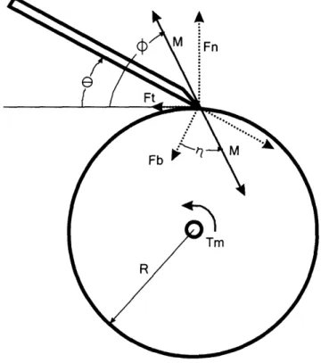
The motor which turns the crucible must have enough torque for the blade to peel the polypyrrole film away from the surface. Figure 10 shows a force diagram of the blade and crucible. In the upcoming analysis, the force required to lift the polypyrrole film will be ignored and simply approximated by a coefficient of friction between the blade and crucible. The minimum torque required by the motor is a function of 0 (the angle of the blade to the surface of the crucible) and u (the coefficient of friction).

Figure 10: Force diagram of peeling mechanism.

The following expression can be derived by equating the applied and reactionary force magnitudes.

F =

cos(9()+ 0 - q~)

where F is the normal force between the blade and the crucible, Fb is the force applied

by the blade to the crucible which depends on the spring tension and length of blade and

is determined experimentally, is angle of the blade to the surface of the crucible, and 0

depends on ,,

0 = cot-_{' (U), (7)}

where u is the simplified coefficient of friction between the blade and the crucible surface. The coefficient of friction varies with each deposition. Sometimes, very thick film depositions have already started to self-separate from the crucible, and other times,

the film is particularly well adhered to surface. It can be assumed that pu does not go

below the coefficient of static friction of dry steel on plexiglass, 0.4, or be larger than that

of rubber on aluminum, 1.0.12 Fb was found experimentally to be about 10 N. Figure 11

shows a plot of minimum motor torque,

Tm =,. Fn*R, (8)

where Tm is the minimum required motor torque to overcome friction, and R is the radius of the crucible. For higher blade angles, the required motor torque increases. For a blade

incidence angle of 25°, the motor should have a torque greater than 0.8 N*m or be geared

down to provide that amount of torque to the crucible.

2I

-

---

-

--

Ok~~~~~~~~'

i

i

~ .... ...Ix~

Blade angle (degrees)

Figure 11: Plot of minimum required motor torque for varying peeling blade angle and coefficient of

friction.

12 http://www.engineersedge.com/coeffientsof friction.htm

3.3 Deposition Control Center Instrumentation and Software

The most important aspect of the continuous deposition experiment is the continuous recording of temperature, voltage, and current data which was accomplished using a Visual Basic .NET program (see Appendix D for the code). The program, called the Deposition Control Center, recorded the measured data and plotted it real time in a graphic user interface shown in Figure 12. The Deposition Control Center also contained

adjustable parameters for the control of the peltiers and the stepper motor.

Figure 12: Screen shot of graphic user interface for the Visual Basic .NET program used to control and

record parameters during a deposition. 3.3.1 Measurements

Temperature measurements were made using Omega precision fine wire thermocouples: Teflon insulated, Type E calibration. Figure 13 shows the locations of the four thermocouples. One thermocouple was placed within the propylene carbonate solution,

one on the cold side of a particular peltier, one on the corresponding hot side, and one in

the air surrounding the machine within the insulated box.

The thermocouples were connected to an Agilent13 _{20 Channel Multiplexer Card 34901A} in an Agilent Data Acquisition/Switch Unit 34970A. Also connected to the 20 channel

multiplexer were two channels containing signals from the AMEL Instruments Power Supply Model 2053 which was used to drive the deposition. One channel described the voltage and the other described the current. The data acquisition unit collected the measurements of voltage for each of the four thermocouples and also recorded the voltage from the current and voltage signals from the power supply.

The measurements were then transferred using a GPIB to USB adapter from the data acquisition unit to a standard PC and recorded by the Microsoft Visual Basic .NET program. The channel which described the current of the AMEL power supply was multiplied by some power of ten depending on the current range which then had to be divided out in the Visual Basic .NET program. That is why there is a field to input current range in the graphic user interface shown in Figure 12.

3.3.2 Controls

A basic proportional integral derivative (PID) control was implemented to control the temperature of the solution. The temperature of the solution was sensed using a thermocouple (see Section 3.3.1). Using .NET, the temperature's present value, present slope, and previous history was evaluated and compared to the desired temperature of -40 C then a command was sent to voltage supplies for the peltier heat pumps. Theoretically the temperature of the solution could be cooled to the desired temperature very quickly with no overshoot, but problems arose with the systems ability to cool the solution (see Section 3.1.1). There was a point when increasing the voltage to the peltier heat pumps would begin to warm the solution instead of cool it. The complexity of the system made the PID control go unstable so it was discarded in favor of basic open loop

control.

3.3.3 Actuators

The Zeta 57-83M stepper motor was driven by a Parker Compumotor 6104 indexer drive which was controlled through a standard RS-232 port on a PC. The ultra slow revolution

13 http://we.home.agilent.com/USeng/home.html

rates required for a deposition meant that the motor would be sent a command to turn a single microstep and wait an interval of a second or two.

The peltiers were driven by open loop control because of the complexity of the system

and the tendency for closed loop control to go unstable (see Section 3.1.1 for an

evaluation of the thermal system).

No other actuators were used in this project, but if the concentrations of reactants were to be actively controlled, a computer controlled injection device would have to be implemented.

4.0 Experimental Procedure

After the machine was constructed and before a deposition was attempted, characterizations of specific functions were performed. After their performance was deemed satisfactory, many full continuous deposition trials were performed with the apparatus and procedure described in Section 4.2.

4.1 System Characterizations

The ability of the peltier/refrigerated-circulator system to cool the solution was analyzed and the accuracy of the stepper motor at ultra slow speeds was examined. It was found that the peltier/ refrigerated-circulator system was not capable of cooling the solution to the desired -40 C. The stepper motor performed exactly as expected and was able to consistently and accurately rotate at speeds slower than one revolution per day.

4.1.1 Peltier/Refrigerated-Circulator System Test

In order to characterize the cooling ability of the peltier/refrigerated-circulator system, thermocouples recorded the temperature at four crucial locations as shown in Figure 14.

T of Peltier hot side

T of Peltier cold side

Figure 13: Diagram of the locations of recorded temperatures (T) within deposition chamber.

The refrigerated-circulator was set to hold the coolant at 0 °C and the system was allowed to reach steady state. Because the coolant gained heat from the environment as it flowed from the refrigerated-circulator through the supply tubes and cooling chamber, the coolant would be warmed by several degrees before it returned to the refrigerated-circulator. Therefore the steady state temperature reached by the thermocouples in the deposition chamber was 5 °C. Figure 14 shows a plot of the four temperatures that were recorded. After the system had been steady for about 200 seconds, the power supplies to the peltier TECs were set to 6 V. The system was allowed to reach steady state again

before increasing the voltage to 7 V, 8 V, and 9 V. The system obtained the lowest

steady state solution temperature of -9 °C at 8 V. At this point, the total current draw of the peltiers was about 23 A which means that 184 W of joule heating was entering the system. The VWR Signature Heated/Refrigerated Circulator, Model 1166 had a rated

cooling capacity of 200 W at 20 °C and 140 W at 0 °C so it is logical that the system

reached steady state at a coolant temperature of about 5 °C.

25

20

--

---

5

---

----

---

- ---

. ---..

_~

E Peltier i Temp Cold

-1 0 --

-twelve peltier l:EPs in parallel.

A perplexing point about the plot is that the temperature of the hot side of the peltier drops when the voltage is supplied. Theoretically the hot side of all the peltiers should increase above the coolant temperature while the cold sides decrease. The strange effect

can be explained by the fact that the coolant entered the right side of the cooling chamber

and warmed up as it flowed to the left. The peltiers at the coolant entrance would create a temperature difference of about -15 C and pass all their heat into the coolant. By the time the coolant got around to the exit, it had warmed up quite a lot. The thermocouples sensed the temperature on a leftmost peltier, as shown in Figure 13, which was kept

colder the cSolnduction than through the internal aluminum box and solution.

-15

i:i

150 350 550 750 950 1150 1350 1550 1750

Time (s)

Figure 14: Plot showing temperatures at the four locations when 6V, 7V, 8V and 9V were applied to the

twelve peltier TECs in parallel.

A perplexing point about the plot is that the temperature of the hot side of the peltier drops when the voltage is supplied. Theoretically the hot side of all the peltiers should

incThe peatier TEC still clreated temperature difference between its hot andwhile the cold decrease. The strange effect, sides but

can be explained by the fact that the coolant entered the right side of the cooling chamber

andjust warmsn't helping as much asto the left. The peltiers near the coolant entrance. Two facts support this conclusion: for one, the recorded temperature for the solaution is lower ath an the

time the coolant got around to the exit, it had warmed up quite a lot. The thermocouples sensed the temperature on a leftmost peltier, as shown in Figure 13, which was kept colder than the coolant by conduction through the internal aluminum box and solution. The peltier TEC still created temperature difference between its hot and cold sides, but just wasn't helping as much as the peltiers near the coolant entrance. Two facts support this conclusion: for one, the recorded temperature for the solution is lower than the

recorded temperature for the peltiers, and two, the air temperature within the insulated box rises significantly as time passes. Also, it was verified that all the peltiers were in the correct orientation and connected correctly to the power supplies. Two sets of six peltiers were connected to single power supply in parallel; therefore each particular peltier could draw varying current depending on its temperature and resistance characteristics.

4.1.2 Stepper Motor Test

The stepper motor was tested because at ultra slow speeds the computer had to wait several second between commands to move a microstep. Tiny mistakes may have added

up to caus large errors. It was found to perform exactly as expected. The stepper motor

was given a command through the Visual Basic .NET program to make 1 revolution in 32 hours. A string was used to keep track of the amount of rotation and after 32 hours, the string had made one complete wind.

4.1.3 Redox Reactions at anode and cathode

The electrodeposition of polypyrrole occurs in an electrolytic cell. A galvanostatic power supply provides the electromotive force. Electrons are pulled away from the pyrrole monomers at the anode creating an oxidized monomer which then connects itself to a

polymer chain. Figure 15 shows diagrams of the generally accepted process of

polypyrrole synthesis. The reaction at the cathode simply produces OH ions and

hydrogen gas.

The TEAP in solution serves two purposes. It breaks into ions which increases the conductivity of the solution. Therefore the voltage which drives the reaction does not

have to be extremely high. The second purpose of the TEAP is that the PF6- negative

ions which have migrated to the positively charged anode become part of the polypyrrole as it is deposited. They do this to neutralize the positively charged pyrrole monomer

chain. For about every three monomers which attach to the chain, one PF6-ion ionically

bonds to the chain. The PF6- ions serve as a dopant in the polypyrrole and ultimately

improve its conductivity.

Syutlhesis of Polypyrrole

IiH

-

-The last step is a in fact a repention of the first steps begiunig with oxidation, followed by coupling to either end of the polymner. and finally elimination of H. The electrons are either removed via an electrode (electrochemcal deposition) or chemlicall. e.g.

Fe+++ e

Fe-Note that the polzmnerization does not generally result in a neutral polymer shown above. but rather the backbone is charged. as below. such that the total mnuber of electrons transferred per monomer

is 2 +a where a is generally between 0.2 and 0.5:

A-

A-where A is an anion or dopant. Here a=l13. Durig fihe iutial phases of electrodepositiol the oholioler. remain in solution. eventually precipitating to form a sohld with intercalated aiois.

Figure 15: Mechanisms of polypyrrole polymerization.'4

14 Taken from Madden, J., Conducting Polymer Actuators, Ph.D. Thesis, Massachusetts Institute of

Technology, Cambridge, MA, September 2000; p. 34.

]

4.1.4 Rate of Deposition

A theoretical high current deposition was simulated using Excel. Various assumptions were used, as shown in Table 2, such as a one to one ratio of pyrrole monomer usage for each electron forced though the circuit by the power supply. In this way, the rate of deposition and decline of reactant concentration could be estimated. The outlined cell boxes were the changeable parameters. Figure 16 and Figure 17 are plots of the estimated number of deposited molecules (proportional to film thickness) and reactant concentrations verses time. Figure 17 shows that the concentration of pyrrole monomer would decrease to 80% of its initial concentration by 600 seconds. This theoretical analysis ignores effects of reactant concentrations on mass transport and diffusion and reaction rates.

Table 2: Theoretical analysis of a high current deposition.

Ppy usage per electron: TEAP usage per Ppy: Ppy mol mass (g/mol): Ppy density (g/mL): TEAP mol mass (g/mol):

Geometry

Surface area of submerged crucible (m2): Rate of rotation

(rot/sec):-Rate of rotation (rot/min):-Rate of production

(m/min):-Experimental Conditions

Applied Current (A)

Initial Concentration of Ppy (M): mL of Ppy added (mL):

Initial Concentration of TEAP (M): Grams of TEAP added (g): Volume of Solution (L):

Calculation Values

Current density (A/m2): Electrons per Coulomb: Electron flow rate (e-/s): Avagadro's Number

Initial number of molecules of Ppy: Initial number of molecules of TEAP:

0.5 0.333333333 67.09 0.967 275.22 0.0110 0.002367424 0.142045455 0.016064489 1.5 0.05 1.734488108 0.05 6.8805 0.5 136.3636364 6.24E+ 18 9.36E+18 6.02E+23 1.51 E+22 1.51 E+22 34 Assumptions

: deposited-- Y TEA~~P - --- --- --- --- . ... -...- ... . .--. ...- . . . .. . .. .. i -i --- --- TA deited --- , --- T---200 300 400 500 600 Time (s)

Figure 16: Plot of amount of molecules that would be deposited on surface of crucible with all assumptions

for a high current deposition.

0.060000 0.050000 c: 0.040000 -O Ca a, ry O 0.030000 - c-0 .O 0 0.010000 -0.000000 0 100 Conci Concentr 200 entration of TEAP (M) ation of Pov (M! 300 Time (s) 400

Figure 17: Plot of concentrations of reactants as time passes with all the assumptions for a high current

deposition 35 3.00E+21 2.50E+21 `0 a) a, -0 a) -2.00E+21 1.50E+21 1.OOE+21 5.OOE+20 0.OOE+00 0 100 500 600 .- ... 4-- . -... I _I -- 11 --- --- I--- I--- --- --- --- --- ---i --- --- I--- I --- i

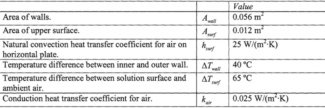
4.2 Experimental Results

The deposition chamber was an anodized 6061 T6 aluminum open-top box, 120 mm square base, 80 mm tall, with 4 mm thick walls. Twelve TE Tech HP-199-1.4-1.15 120 W peltier thermoelectric coolers surrounded the box and were in contact with anodized aluminum walls with serpentine channels containing coolant of 50% water and 50% Glycol from Alfa Aesar. On top of the cooling chamber rested a lid which held a glassy carbon crucible down inside the deposition chamber. The crucible was supported on an axle on two ABEC 5 bearings and could be rotated by a Zeta 57-83 Stepper Motor driven

by a Parker'5 Compumotor 6104 indexer drive. The lid also sported a peeling mechanism

which consisted of two standard razor blades pressed against the crucible using spring tension. The deposition chamber and lid with crucible and peeling mechanism are shown

in Figure 18.

Figure 18: The completed cooling chamber and peeling mechanism.

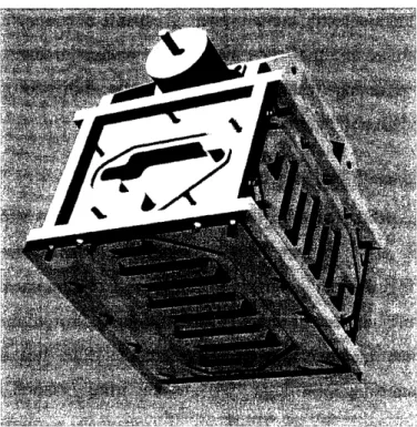
The deposition chamber sat within a thermally insulating Styrofoam box which is shown

in the photo of the entire experimental set-up in Figure 19. A VWR16 Signature

Heated/Refrigerated Circulator Model 1166, with a two-speed pump and 6 L bath cooled the coolant and circulated it through the serpentine channels in the cooling chamber.

36 5IS http://www.compumotor.corm/

Two Hewlett Packard ?System DC Power Supplies, one Model 6653A 0 V to 35 V, 0 A

to 15 A and one Model 6652A 0 V to 20 V, 0 A to 25 A, provided the power to the

twelve peltier TECs. An AMEL Instruments Power Supply Model 2053 was used to provide current and voltage to drive the reaction

Figure 19: Photo of entire experimental set-up which includes three power supplies, a chiller/circulator, a

data-acquisition unit connected to a standard PC, and the deposition chamber within the insulating box.

Temperature measurements were made using Omega precision fine wire thermocouples:

Teflon insulated, Type E calibration, 1 m long, and 0.127 mm diameter. The

thermocouples were connected to an Agilent 20 Channel Multiplexer Card 34901A in an Agilent Data Acquisition/Switch Unit 34970A. The data acquisition unit also recorded the current and voltage signals from the AMEL Instruments Power Supply. The measurements were then transferred using a GPIB to USB adapter from the data acquisition unit to a standard PC and recorded by the Microsoft Visual Basic .NET program.

4.2.1 Methods

Before beginning a continuous deposition, the crucible was well cleaned with acetone. If

the surface was damaged after 3 to 5 repeated uses, it was polished using a Divine Dico

37

E-5 emery composition for hard metals rouge stick. The copper counter-electrode sheet

was detamrnished using Cameo copper, brass and porcelain cleaner

The propylene carbonate solution was prepared with 0.05 M tetraethylammonium hexaflourophosphate (TEAP) and 0.05 M pyrrole monomer, which were the same concentrations used in batch-productions. 7.5686 grams of TEAP and 1.9793 mL of pyrrole monomer were added to 550 mL of propylene carbonate. The pyrrole monomer must be stored in a nitrogen environment and in a freezer to prevent oxidation and other reactions. After the pyrrole was added to the propylene carbonate solution, nitrogen was bubbled into the solution, and then the beaker was covered with parafilm and placed in a

freezer.

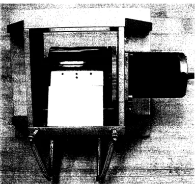
The refrigerator/circulator was set to 0 C and turned on and the system was allowed to

reach a steady state temperature. The Deposition Control Center program (Section 3.3) was initiated and began recording data points at 30 second intervals. Then, with the lid and crucible removed, the solution was poured into the deposition chamber and a voltage

of 5 V was applied to the peltiers. Figure 20 shows the deposition chamber after the

solution has been poured in and the copper counter electrode put into place.

Figure 20: Photo of cooling deposition chamber containing solution and with copper counter-electrode

installed.

The lid and crucible were put into place. The positive terminal from the AMEL power supply was clipped to the copper counter-electrode, the negative terminal was clipped to the peeling device which was in contact with the crucible through the blade. The

electrodeposition was run under galvanostatic control at a current density of 0.5 A/m2.

The crucible has only 0.011 m2 of surface area on the bottom half which is below the

solution level so the AMEL power supply was set to a constant 5 mA.

Using the Deposition Control Center program, the stepper motor was set to make 2 revolutions in 64 hours and all temperatures and voltage and current data were recorded every 30 seconds. The experiment was checked periodically to make sure no malfunction occurred.

5.0 Results and Discussion

5.1 Typical Deposition

Many full continuous deposition trials were performed; although, since no reactant addition devices were implemented, the maximum length of time for a trial was under 72 hours. Figure 21 shows plots of typical data for a trial. The solution temperature was

maintained at a relatively stable -10 °C. The wavelike shape of the temperature plot is a

result of room temperature variation throughout a day - one period in 24 hours,

5 0 -5 -10 -15 20 10 0 -10 -20 IU 5 0 0 5 10 15 20 25 30 35 40 4: Time (h) ,, . . : _ ... . .' ...:. .. ... ...i ... : ... ... ... . ... ... ... ... ... ,...

...

Figure 21: Typical plot of recorded values of solution temperature and the electrode voltage and current for a full continuous deposition trial.

The power supply was set to hold a constant 5 mA and transferred 792 C of charge in 44 hours. The typical, initial 4.5 V potential between the electrodes was several volts higher than expected from batch-deposition with the same current density. The higher potential was caused by higher resistance in the electrodeposition circuit. The spikes in electrode

40 I - l I l 1 I I : i : : ... . . . : . . . .. . . : . ... . . . .. . . . ... ... . . . . . . . i I i i a) a) 2. E a) 8. U -Cu , 0cm v o 0_'a m. (D C 0 a) 0 a) .. . - . .. . .. .. . .. .. . .. . . ... .. : ... . .. ... .. . ... . .. .. : .. .. ... .. . .. . I. I . .. i i I I - I

voltage that occurs at about 7.5 hours is associated with the blade beginning to peal the first polypyrrole from the crucible. When the resistance of the circuit changed because of poor blade contact with the crucible, the driving voltage had to adjust. The repetitive small peaks that follow are explained by the fact the stepper motor did not have enough torque to peal the polypyrrole film off of the crucible. The stepper motor would take micro steps until the reverse force was too great and and the stepper motor would be forced to jump one whole step in reverse, then the cycle would repeat. This means that

the crucible stayed in the same position from 7.5 hours onwards.

The film deposition that results from a trial during which the stepper motor failed looks like the one shown in Figure 22. A section of the crucible was beneath the surface of the propylene carbonate solution for many hours while the crucible was stationary and the reaction-driving current was still applied. This section of film began to bubble and separate from the crucible. One possible reason for the film separation is the degradation of the polymer by continued application of current while submerged in propylene carbonate - a phenomenon that has been witnessed during the testing of polypyrrole as an actuator. The precise method of polymer attachment to the crucible surface is not completely understood. The polymer strands might form in solution then "settle" onto the surface of the crucible. Varying degrees of peeling difficulty are experienced and could be a function of many variables such as temperature. The crucible and polypyrrole have different coefficients of thermal expansion and so when the section of the crucible

in the ambient air has warmed to 25 °C from the -10 °C, the film may have already started to separate from the surface.

Figure 22: Photo of deposition during which the stepper motor failed to turn. The film on the bottom half

of the crucible bubbled and began to separate from the surface.

A deposition was run with manual help to initiate peeling and a piece of polypyrrole almost 50 mm long and 70 mm wide was successfully produced. Figure 23 shows the polypyrrole being peeled off of the crucible. Once the peeling was started by hand, the stepper motor was easily able to perform the rest. Figure 24 shows the piece of polypyrrole that was produced. The side displayed was the side which touched the surface of the crucible and was more glossy than the side formed facing the solution. The piece of film was 0.246 mm in the thickest area - over three times thicker than a typical

batch-deposition run for the same length of time and current density. The greater

thickness could be a result of the deposition occurring at -10 °C instead of -40 °C because reaction rates increase with temperature.

Figure 23: Photo of a successful deposition. The blade has started peeling the polypyrrole off of the crucible.

Figure 24: Photo of a piece of produced polypyrrole.

A section of the polymer was cut 2 mm wide and 60 mm long. It was found to have a conductivity of 1.4x 104 S/m. Copper has a conductivity on the order of 107 S/m and a material with a conductivity below 10-8 is considered an insulator. The best conductivity

of polypyrrole produced in the MIT BiLab was 5 x 104 S/m. The piece was tested using a

Perkin Elmer Dynamic Mechanical Analyzer 7e (DMA). The results shown in Figure 25 show that the Young's modulus was 0.29 GPa for low strain and 74 MPa for high strain. The sample was not taken to the failure point because the DMA reached its maximum force output. At 8% strain the 2 mm wide sample held a load of almost 7 N.

li HE I I i I I fi b 11 .1 Hi i fi I I = ~~~~~~~~~~~~~X

& le .dt Sew Esya curves ath Calc Ioeb tr sw etilp

--- - --- 1S l --ic ISe --- , -- . - - -e ,, Strain Probe Posi tI Am , - , 1 m 1e-,

I Static tmes -l 18tatl'~o- -| P07Mctrin1 -l Pob.Posifi.o -| imltd ||apeep - Soaeouu-

REMM ____ a~p, ~ _

DMA 7e r ...

Slope = 74338e+007 Pa Inverse Slope = 1.34521e-00 1/Pa

3- -- -- - -- -- ---

-/Slope = 2.9404e+008 Pa Itverse Slope = 3.40O90e-009 1Pa

I, . i . i i i~~~~~~~~~~~~~~~~~~~~~~~~~~~~~~~~~~~~~~~~~~~~~~~~~~~~~~~~~~~~~~~~~~ i L~~~~~~~~~~~~~~~~~~~~~~~~~~~~~~~~~~~~~~~~~~~~~~~~~~~~~~~~~~~~~~~~~ 3 4 Static Strain (%) Probe Weight: to0.131

Figure 25: Screenshot of the stress-strain results of DMA test of 2 mm wide sample of polypyrrole.

5.2 High Rate Deposition

Several high rate depositions were performed. The same procedure as described in Section 4.2.1 was followed except 1.5 A instead of 5 mA was used to drive the reaction and the stepper motor was run at 1 revolution per 4 minutes instead of 1 revolution per 32

44 1 .534e,7 1 .400e+7 1.200e+7 1 .000e+7 8000000 S 6000000 4000000 2000000 Axis: x-. 3295 % Cottd Panel R IX-E 156, ' C Purge Ges, Nit. ege i 20.0 mmn Apply | y -- 1.7e+6P y - -1 .0107e+006 P. 6 7 8 8.613 i I i i i i i 2 Is

hours. Higher current would have been used, but the AMEL power supply had reached its maximum power output. The idea for high rate deposition came from a journal article

on the industrial polypyrrole deposition on zinc-electroplated steel8. The study had

shown that 2 ,tm of polypyrrole could be deposited in 1 s with a current density of 7000

2

A/m2.

During all the high rate depositions, the film created on the surface of the crucible was very powdery - not much a film at all - and the propylene carbonate solution turned from clear to black. Both of these observations suggest that the pyrrole monomer was over-oxidized. Side reactions occurred and polymer chains were cut short. The solution turned black because short pyrrole oligomes diffused back into solution after over-oxidation.

18 E. Hermelin, J. Petitjean, S. Aeiyach, J.C. Lacroix, P.C. Lacaze, Journal of Applied Electrochemistry 31

(2001) 905-911.

6.0 Conclusion

In order to produce conducting polymer in larger quantities and higher quality and repeatability, a prototype for a device was designed, built and tested. The device successfully produced a thick polypyrrole film 50 mm by 70 mm with mechanical properties comparable to typical batch-produced polypyrrole at the MIT BiLab. Longer pieces were not produced because the stepper motor was too weak for the peeling mechanism to work. A few high-rate depositions were attempted, but failed - most likely due to over-oxidation preventing the formation of long polymer strands. More research should be performed on depositions with current densities over 300 times typical batch depositions to explore the possibilities and qualities of quickly produced polymer.

7.0 Future Work

A second prototype of this machine should be designed with improvements based on what was learned from the first prototype.

* Apply more torque to the rotating crucible. The use of a gear box to gear down the stepper motor would both increase the motors resolution and torque so that it was strong enough to initiate peeling of the polypyrrole film from the crucible. * Use more effective and more efficient cooling device. A liquid to liquid heat

exchanger and placing the deposition chamber in heat transfer fluid would eliminate the inefficiencies of multi-stage cooling

* Direct connection to working electrode. The first prototype used the peeling blade to make contact with the rotating working electrode. The blades corroded quickly because of the current running through them. The uncertain contact between blades and crucible surface caused spikes in resistance. A free spinning direct wire attachment would allow the crucible to turn while still providing a non-corroding, direct electrical contact.

* Actively control reactant concentrations. The use of powered syringes or gravity and computer actuated valves to add precise amounts of reactants would make it possible to keep reactant concentrations constant for long depositions.

* Measure hydrogen ion concentration. The propylene carbonate solution is only 1% water so pH does not really apply and typical electronic pH sensors do not work below -5 C because the impedance of glass gets too high. The hydrogen

ion concentration could be measured using an Oxygen-Reduction Potential (ORP) platinum electrode like the Beckman 511120 12x 150 mm. Although the absolute

value of [H+] would not be known, the change could be measured and

counteracted.

* Easy to clean. All parts should be simple and designed with thought to how they can be cleaned

* Plastic parts where possible. Using plastic instead of metals whenever possible would eliminate unwanted electric fields and short circuits. It would also help cleanability. Attention must be given to use plastics which resist the chemicals used.

* Beware of hydrogen gas production. Some of the depositions may have failed because of hydrogen gas formed at the counter electrode and rose up through the solution to hit the working electrode. A screen could be installed between the two electrodes which allows the passing of ions, but deflected the hydrogen gas. In a typical batch-deposition, the crucible and counter electrode are vertical so the gas

is not a problem.

Figure 26 shows a sketch of a proposed second prototype. The idea uses a smaller glassy carbon crucible so that solution quantities are smaller and also so high current density depositions could be performed with a typical power supply. The gear box tower will give the stepper motor plenty of torque at the crucible. The large volumes in the deposition chamber to the left and right of the crucible give room for reactant concentration measurement and control. The entire chamber will sit in a liquid to liquid chiller bath.

-1r l I,.'

A

Z

Figure 26: Sketch of proposed second prototype.

48 I I -- '1---.I-- - - -- --- --- --- --- , --- --- -- - -- I

References

[1] Hermelin E., Petitjean J., Aeiyach S., Lacroix J.C., Lacaze P.C., Journal of Applied

Electrochemistry 31 (2001) 905-911.

[2] Lu, S.L., Yang, M.J., Luo, J., Cao, Y., Sythnthetic Metals 140 (2-3): 199-202 FEB 27

2004

[3] Madden, J., Conducting Polymer Actuators, Ph.D. Thesis, Massachusetts Institute of Technology, Cambridge, MA, September 2000.

[4] Rinderknecht, D., Design of a Dynamic Mechanical Analyzer for the Active Characterization of Conducting Polymer Actuators, Cambridge, MA, June 2002.

[5] Riul, A., de Sousa, H.C., Malmegrim, R.R., dos Santos, D.S., Carvalho, A.C.P.L.F.,

Fonseca, F.J.., Oliveira, O.N., Mattoso, L.H.C. Sensors and Actuators B-Chemical 98 (1):

77-82 MAR 1 2004

[6] Schmid, Bryan, Device Design and Mechanical Modeling of Conducting Polymer Actuators, B.S. Thesis, Massachusetts Institute of Technology, Cambridge, MA, June

2003.

[7] Yamato, H., Kai, K., Ohwa, M., Asakura, T., Koshiba, T., Wemrnet, W., Sythetic

Metals 83 (1996) 125-130.

Appendix A- Polypyrrole Batch-deposition Method

Materials:

- Glassy Carbon Crucible - Peter Madden's Lathe Mount - Jeweler's Rouge

- Copper Sheet (Counter Electrode) - Fine Sandpaper

- Plastic Wrap - Stir Magnet

- Stir Magnet Removal Rod - Crucible Centering Cap - Potentiostat

- BNC to dual banana plug converter - BNC cable

- BNC to alligator clips cable

- -40 °C Refrigeration Unit and Cooler - 1L Beaker

- Solutions:

Propylene Carbonate

TEAP (tetra-ethylammonium hexafluorophosphate) Distilled Water

Pyrrole Monomer

Method of Preparation:

- Turn on refrigeration unit

- Prepare the first fraction of the pyrrole solution in 1 L beaker

o 0.05 M PC (propylene carbonate)

o 0.05 M TEAP (tetra-ethylammonium hexafluorophosphate) o 1% vol. H20 (distilled water)

- Cover the beaker with plastic wrap then place it in the refrigeration cooler

- Wash crucible with acetone

- Polish crucible with jeweler's rouge on lathe using lathe mount

- De-tarnish copper counter-electrode with fine sandpaper

- Following steps should be done as quickly as possible to prevent, as much as

possible, excessive temperature rise in the solution

o Remove Pyrrole monomer from its stock tube using a disposable syringe o Remove beaker from cooler, allowing the coolant to drip off as much as

possible then keeping it ion a paper towel