Current distribution in cable-in conduit superconductors
Texte intégral
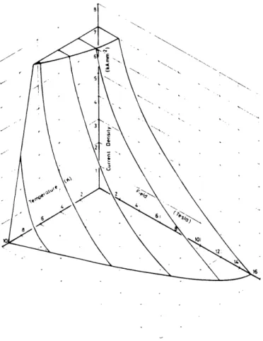
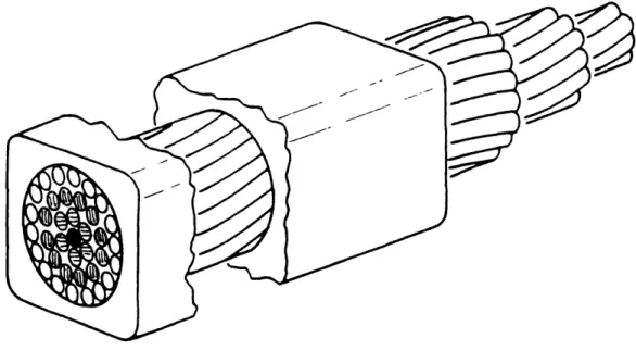
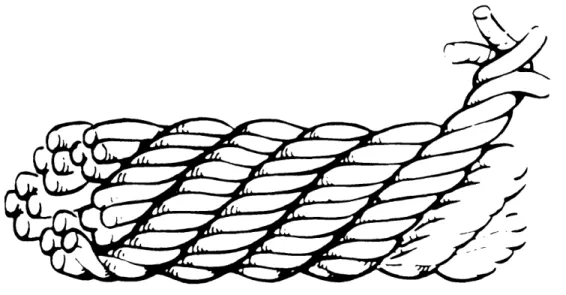
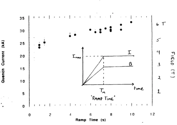
Figure


Documents relatifs
We consider the problem of Diophantine approx- imation on semisimple algebraic groups by rational points with restricted numerators and denominators and establish a quanti-
1 Anthony Babkine et Adrien Rosier, Réussir l’organisation d’un événement , croupe Eyrolles 2011,P2.. ~ 29 ~ : ةساردلا جهنم و هيلع فرعتلاو
Continuous Closed Form Trajectories Generation and Control of Redundantly Actuated Parallel Kinematic Manipulators.. SSD: Systems, Signals and Devices, Feb
Therefore, particles with large diameters (and, subsequently, long pore channels), are capable of demonstrating high capacitance and ion dynamics. In addition to a good
(French) [Riesz transforms for Gaussian laws]. Vector-valued Singular Integral Operators with Non-smooth Kernels and Related Multilinear Commutators. Pure and Appl. A geometric
In this study, 4% betaine treatment induced cell cycle arrest in G 2 /M phase, preventing a further proliferation of cancer cells, as similarly observed in HeLa cells [35],
Le Conseil d’État admettait la possibilité pour le justiciable d’introduire une action en justice sans lier le contentieux, donc en l’absence d’une décision
d’informations relatives à l’adrénochrome en décrivant cette substance simplement comme le pigment obtenu après oxydation de l’adrénaline : elle n’est d’ailleurs pas
