Credibility Approximations for Bayesian Prediction of Second Moments

SECOND MOMENTS BY WILLIAM S. JEWELL*

University of California, Berkeley, California

AND

RENE ScHNiEPERt

Department of Mathematics, ETH-Zentrum, Zurich

ABSTRACT

Credibility theory refers to the use of linear least-squares theory to approximate the Bayesian forecast of the mean of a future observation; families are known where the credibility formula is exact Bayesian. Second-moment forecasts are also of interest, for example, in assessing the precision of the mean estimate. For some of these same families, the second-moment forecast is exact in linear and quadratic functions of the sample mean. On the other hand, for the normal distribution with normal-gamma prior on the mean and variance, the exact forecast of the variance is a linear function of the sample variance and the squared deviation of the sample mean from the prior mean. Buhlmann has given a credibility approximation to the variance in terms of the sample mean and sample variance.

In this paper, we present a unified approach to estimating both first and second moments of future observations using linear functions of the sample mean and two sample second moments; the resulting least-squares analysis requires the solution of a 3 x 3 linear system, using 11 prior moments from the collective and giving joint predictions of all moments of interest. Previously developed special cases follow immediately. For many analytic models of interest, 3-dimensional joint prediction is significantly better than independent forecasts using the "natural" statistics for each moment when the number of samples is small. However, the expected squared-errors of the forecasts become comparable as the sample size increases.

0. INTRODUCTION

In applications of Bayesian prediction, it is often difficult or extravagant to compute the entire predictive distribution; for example, the underlying likelihood and prior densities may be empirical, with only a few moments known with any degree of reliability. Also, the decision structure may depend only upon the first few moments, instead of upon the total shape of the predictive density. Finally,

* This research has been partially supported by the Air Force Office of Scientific Research (AFSC), USAF, under Grant AFOSR-81-0122 with the University of California.

t The research was supported by a grant from the Swiss National Science Foundation.

the need for repeated recalculation of forecasting formulae may argue for simple, easy-to-compute results.

A case in point is actuarial science, where the fair premium (predictive mean) is the point estimator of basic importance. To this may be added fluctuation

loadings, which are given functions of the predictive second moment, the variance,

or the standard deviation (see, e.g., GERBER, 1980). Credibility theory is the name given by actuaries to approximations of Bayesian predictors by formulae that are linear in the data, chosen to minimize quadratic Bayes risk. Thus, credibility

formulae are linear least-squares predictors, and are akin to the classical estimators

of that type, and to the linear niters used in electrical engineering.

The main emphasis of credibility theory thus far has been on approximating the predictive mean, under a wide variety of different model assumptions (see,

inter alia, NORBERG, 1979; JEWELL, 1980). For many simple models used in practice, the linear credibility predictor of the mean is exactly the Bayesian conditional mean; in other situations, the credibility formula is usually quite robust.

1. BASIC MODEL AND NOTATION

Consider the usual Bayesian setup, in which a random observable, x, depends upon an unknown parameter, 6, through a (discrete or continuous) likelihood

density, p(x\6). In the experiment of interest, 0 is fixed at some unknown and

unobservable value 0, but the parameter has a known prior density, p(d). The conditional moments of JC, given 6 are:

If we were to attempt to predict x prior to observing any data, and without knowing 0, we would have to use the marginal density of x, p(x) = %{p{x\0)} = jp(x\d)p(0) dd, which has prior-to-data (marginal) moments:

(1.2) mi=^{mi(d)}=n(x)i}.

For convenience in the sequel, we also define higher order cross-moments about the origin, such as:

(1.3) mv=<g{mt(e)mJ{e)}\ mijk=<g{mi(e)mj(d)mk(e)}; etc.,

explicitly permitting the indices to be repeated, e.g., mn=^{(mt(6))2}. Thus,

from the four conditional moments {m^d); i = 1,2,3,4} we can form eleven marginal moments of order four or less:

(1.4) M = {mx; m2, mu; m3, m21, mlu; m4, m31, m22, m2n, ml u l} . Three central moments of order two deserve special symbols: (1.5) e=%T{x\0} = m2-mn; d = Tg{x\0}=mll-m21;

where double operators and their corresponding operands are to be interpreted "inside-out". Central moments of higher order can also be defined.

Now suppose that n independent observations, 2 = {xu x2,..., *„}, are drawn

from the same likelihood density, p(x\ 6), with 6 fixed, but unknown. From Bayes' law, the posterior-to-data parameter density is:

(1.6) P(6\2))K ft P(x

u

\d)p(d),

u = l

and knowing this enables us to calculate the posterior-to-data predictive density for the next observation, *„+,, as:

(1.7) P(xn+1\3) = j p(xn+1\0)p(O\2) dd.

This is, in fact, the predictive density for any future observation, assuming that

6 does not change, and that no more information is available. From our viewpoint,

given % the {*„+,, xn+2, xn+3,...} are exchangeable random variables; for example,

the joint predictive density of (xn+1, xn+2) is:

(1.8) P(xn+uxn+2\3))=\ P(xn+l\d)p(xn+2\e)p(e\2)) do.

(1.7) and (1.8) also have predictive moments analogous to (1.2), (1.3): (1.9) m,(®) = %{xn+1\!2)}; m2{2)= ^{x2n+l\3>};

mu(2>)=%{xn+lxn+2\2)}; etc.,

that can, in principle, be calculated exactly; however, analytic solutions almost always require that p(x\0) and p(6) be chosen from among natural conjugate

families. We now consider how approximate results can be obtained for the

predictive moments in (1.9).

2. CREDIBLE MEAN FORMULAE

Consider first the problem of calculating or approximating m^Sb). For many years, actuaries (in a different terminology) have been assuming that this "experience-rated premium" was linear in the data, as summarized in the sample mean, x = £ xu/ n (it is clear from exchangeability arguments that each of the samples, xu, should be weighted the same). Using heuristic reasoning, they argued

for the approximation:

i.e., the forecast, f*{3)), should be a convex combination of the "manual" (prior) mean, m,, and the "experienced" mean, x. The "credibility factor", zu that

weights these two means is, they argued:

where the "credibility time constant", nou was to be chosen empirically. This

heuristic formula, used for many years, was considerably strengthened by

BUHLMANN (1967), who showed that the best linear formula (in the least-squares sense) to approximate the predictive mean mt(3i) was precisely the credibility

formula, f*{3>), but with the time constant computed explicitly from the prior second moments:

, . , , e m2-mu m2-mx c

a mn — m\ mu — m\ a

Thus, a credibility predictor to approximate %{xn+1\3)} needs only the first three

components of (1.4), {ml; m2, mn}, instead of the complete shape of the prior

and likelihood densities.

In fact, Bailey, Mayerson, and others had already shown in the 1950s that (2.1), (2.2), (2.3) was exactly mx{3)) for many "natural" p{x\8) and p(6) used

in Bayesian modelling. JEWELL (1974a) then showed that, if the likelihood were a member of the simple exponential family (for which x is the sufficient statistic) over some space

x-(2-4) p(x\e) = a{X^e0)0X, (xeX)

and p{8) were the natural conjugate prior to (2.4):

°l e~ex°>

over the maximal range © for which the normalization g{nou xm) is finite, then,

under a certain regularity condition (JEWELL, 1975), (2.1) is exact, with the hyperparameters n01 in (2.3) and (2.5) identical, and with xOi = minOi.

A simple, argument also shows that, if the exponent 6x in (2.4) is replaced by, say, 6t(x), then the credibility form (2.1) again provides an exact prediction for ${f(xn+1)|2)} as a linear combination of the prior mean of the statistic, %{t(x)}, and the sample mean of the statistic £ t(xu)/n, with appropriate redefinition of

(2.3). For this and other reasons that will become clearer below, we feel that (2.1) is a robust formula in most cases.

3. EXACT RESULTS FOR SECOND MOMENTS

We now consider exact results that are known for the predictive moments, m^®), m2(2>), and mu(3)), concentrating on the most-studied case, the simple

exponen-tial family.

It is well known that the combination (2.4), (2.5) is closed under sampling, so that, posterior-to-data 2, the hyperparameters in (2.5) are replaced by:

Since m, = XOI/MOI, it follows that the updated first moment is:

(3.2) 9{xH+l\ai}=

which is simply (2.1), (2.2). It is also clear that the marginal second moments must also involve only n01 and x01, and that the predictive second moments must be a function of only the sufficient statistic, x, but no further statement can be made about dependencies in general. JEWELL (1974a) tabulates d = d(nou xm)

for six of the examples given below, whence one can easily get e = nold(nou x01), c = (no+ l)d(nOi, xOi), and hence:

(3.3) m2(®) = (n0, + 1 + n)d(n0l + n, x01

mu(2s) = d(nOi + n, x0l + nx)

and, from these, the updated versions of the central moments c and d;.

(3.4) 2

EXAMPLE 1. Let p(x\0) be Bernoulli (TT) and p(ir) be Beta (x01, «oi-^oi). (6> = l n ( 7 r '1- l ) ) , then:

( 3

-5 ) < *( H X ) =

EXAMPLE 2. Let p(x\0) be Geometric (IT), and p(ir) be Beta (xol, nol + l),

= lnir~1), then:

(3.6)

EXAMPLE 3. Let p(x\6) be Poisson (TT) and p(ir) be Gamma (xou n01), (6 =

In TT~l), then:

(3.7) (

0U0l

) f

EXAMPLE 4. Let p(x\6) be Exponential (6), andp(6) be Gamma (n0i + l,x0 1), then:

(3-8) /0 1

EXAMPLE 5. Let /?(x|0) be Normal (TT, si), si known, and p(n)~

Normal (xOi/nOi, *o/«oi), 0 = -ir/s%, then:

(3.9) d(n0l, xOi)=—^ (independent of x01).

Thus, in these examples from JEWELL (1974a), d(nou x0l), m^Sd), m2{£b), and mn(3)) are all linear, quadratic, or constant in x01 and hence in x as well.

MORRIS (1982) refers to simple exponential likelihoods (2.4) in which m2(0)

is at most a quadratic polynomial in m^O) as QVF-NEF; he shows that the only members of this family are the five examples above, plus Example 6, below, plus all of the related members found through linear translation and convolution (Binomial, Pascal, Gamma, etc.).

EXAMPLE 6. The last member of this group is the Hyperbolic Secant density:

for which

(3.10) d(nol,xol) =

This likelihood seems to be useful only in certain random-walk problems. We should mention also that it is easy to construct members of the simple exponential family in which the mean is a complicated function of x, for example, by truncating the range of any of the above distributions.

To obtain dependency on x and other statistics, we must turn to two-parameter families, of which the most popular is the normal density with both the mean, /I, and the precision, i3, as random quantities.

EXAMPLE 7. Let

p(x\d) = p(x\fi, ay) = Normal (/u., co'1)

p(w) = Gamma I and

Ix

\

p(fi\a>) = Normal I — , (n0lw)~l ,

\«oi /

with a, x01, x02, and n01 given hyperparameters. This family is closed under sampling, with updating:

(3.11) a<-a+-; nol*-noi + n;

from which we find that (3.2) again holds, and that:

(3.12) d ( 0 1 , , o l , 0 2 ) ^ \ )

( 2 a - 2 ) L \ « o i / \noi where c = e + d is the prior variance.

For this example, we see that the updating jvill give exact second-moment predictors that are quadratic in x and linear in x2 = £ x2j n. Because the normal

case is so important to least-squares approximations, we also give the exact results corresponding to (3.4) in terms of the sample variance, s2= n"1 £ (xu — x)2, the

sample mean, x, the prior marginal variance, c, and the credibility factor, z,: (3.13) nxn+1\2)}

2a -2+n

An important simplification occurs if the "natural" choice 2a = n0l + 3 is made;

note that this does not significantly restrict the choice of the 2-parameter Gamma, but does mean that there are only three distinct hyperparameters in all. (3.13) then simplifies to a generalized credibility formula:

(3.14) Y{xn+l\®} = («oi +1 + n)<€{xn+l; xn+2\9}

This result is not new, but rearrangement into credibility form first appeared in

JEWELL (1974a). The equivalent multidimensional formula appeared in JEWELL

(1974b, 1983).

(3.14) is, in fact, equivalent to:

(3.15) %{x2n+m = m2(2) = (l-z1)m2+ z,72,

that is, the predictive second moment is exactly in credibility form with the same credibility factor as in (2.2), with obvious adjustments to the prior mean and sample mean.

4. LEAST-SQUARES THEORY AND MULTIDIMENSIONAL CREDIBILITY We now take a temporary detour to display some general results from multi-dimensional credibility theory that will be used in the next section. Suppose we have a vector-valued version of the Bayesian model of Section 1, in which samples ® = {)>n )>2, • • •, yn} of a vector-valued random variable, y, are to be used to predict

a random vector, w. If we approximate ${M>|®} by a linear function of the vector-valued sample mean, y=J,yn/n, least-squares theory then shows that the

best (vector-valued) predictor is: (4.1)

where Z is a matrix of appropriate dimensions given by the solution of the normal

system of equations:

(4.2) zny;y} = n*;y}

{<€ is the matrix covariance operator).

Now suppose w is actually a future observation of the same random vector,

y, say w = yn+1. Then these equations become:

(4.1')

where / is t h e nxn unit matrix, Z is t h e square solution of:

(4.2')

m is the prior mean vector, obtained from the conditional mean vector:

(4.3) m(6)=%{y\0};

and E and D are the two components of within-risk and between-risk covariance, respectively:

(4.4) E=WV{y;y\S}; D = 8

Thus, the credibility formula of Section 2 extends directly to the multi-dimensional case, with a credibility matrix, Z, mixing the prior mean, m, and the experience mean, y. The analogy is complete if we assume D has an inverse and rearrange (4.2'):

(4.5) Z=nD(E + nDyl = n(nI + Nyl; 1W = ED\

where JV is now a matrix of time constants. Further details on this extension may be found in JEWELL (1974b).

The accuracy of any forecast / ( 2 ) for yn+l is measured by the diagonal terms

of the expected squared-error matrix: (4.6) • *

note that the expectation is over all possible joint values of (yn+i; 3>). However,

since the latter are independent, given 0, <& can be decomposed into: (4.6') *=WKyn+i-m(0)Iyn+1-m(5m+ £{[/(©)-m(0)][/(@)-m(0)]'}

= E + V, say,

where we see the portion of the mse due to the inherent fluctuation of the observable, and the mse due to the approximation of the true mean, m(0), by the approximation, f{3)).

We know that the minimum values of the diagonal terms for <I> and *P are attained by picking the Bayesian predictive mean, m(3)) = ?{J7n+1|2>}, which, in general, leads to a nonlinear regression on the data. With a linear forecast (4.1'), (4.2'), it is easy to show that, for any n,

In most eases of interest, all terms of ^ will approach zero as n approaches infinity for any forecast, so that all forecasts are asymptotically equivalent; in the linear case, it usually happens because Z approaches I (see also (8.6)). Fortunately, a linear predictor also usually has small mean-squared-error also for moderate n, even though f{3>) is not exactly the Bayesian predictive mean. We now examine the use of (4.1'), (4.2') as an approximation for our original one-dimensional problem of estimating second moments.

5. ORGANIZING THE LEAST-SQUARES COMPUTATIONS

We return to the main problem of organizing credibility approximations f2{3>)

a n d /u( 2 ) ) for m2{2) and mn(3>) of arbitrary distributions. In view of the exact

results in Section 3, it seems reasonable to restrict the statistics to be used to linear and quadratic functions of the data; however, there are several different ways to select statistics of this type. After a great deal of experimentation, the authors have found that the choices that give the simplest and clearest results are the "natural" first and second moments about the origin:

(5.1)

(

3

)

I , ;

I

( 2 ) ) l

2

( ) I l ;

~

2 1 1

^

( )

7

n n

n(n-for «5*2. In other words, v/e set y = [t1(2});t2(3));tn(2))']' = t(2)) in (4.1). Note

that this choice implicitly includes (x)2 = [t2(3)) + (n - l)tu(2d)y n, as well as the

sample variance s2 = [(n-l)/nj_t2(3))- tu(2)~\.

As predictands, we can get all the forecasts of interest simultaneously by setting

w = [xn+l; x2n+1; xB+1xn+2]'. Then, to get Z in (4.1), we need only to compute the means in (4.1) and the two covariance matrices in (4.2). This approach is thus similar to credibility regression modelling; see HACHEMEISTER (1974).

For the means, we find easily: (5.2)

%{y}=%{w} = m=[ml; m2; mnj.

(Note that mu(6) = m2(6).) Computation of the covariance terms is

straightfor-ward, but tedious, as they involve all 11 moments of (1.4); we find, for n & 2 : (5.3) {yy}

n

where D and E{n) are new matrices, analogous to the matrices in (4.4), but otherwise unrelated. Explicitly, we find:

(5.4) D =

i ~ nil m2\ —m2ni\ mm — nt m22 —m2 m2\\ —YTI

and (5.5) where (5.6) and (5.7) E,; Eao = n-\ m2 — mu m3 — m21 m4-m22 2(m3 1-m2 n) (symmetric) 4 ( m2 n- w ii m) 0 0 0 0 0 0 0 0 2(m2 2-2m2,r

Once these have been computed, the credibility matrix Z is the solution of: (5.8) z(D+-E(n))=D;

and the vector forecast /(2>)=[/i(2));/2(2>);/u(®)]' is given by:

which should be compared with (4.1'), (4.2').

6. INDEPENDENT FORECASTS USING NATURAL STATISTICS

Before examining the various aspects of the three-dimensional forecast (5.9), it is of interest to consider first how the one-dimensional result (2.1) would general-ize if second-moment forecasts were made only in terms of their "natural" statistics, i.e., if the solution to Z were forced to be diagonal. We find:

(6.1) r, z , = " 0 2 + « ' m4 - m22 m22 -m2 rim —" and, for n 3= 2, (6.2) m 4(m2 n-mn i l) + n + nou(n)' i-m2_u

These are to be compared with (2.1), (2.2), (2.3), which, of course, still hold for the first-moment forecast. (Note that asterisks distinguish the independent forecasts/f,/*, and/fi from the corresponding components of the joint forecast

/ and that zu in (6.2) is not the (1, l)st component of Z in (4.2').) We will return to analysis of independent forecasts in Section 9, after analyzing the asymptotic behaviors of (5.8), (5.9).

7. LIMITING BEHAVIOR OF THE JOINT FORECAST

The analogy with (4.5) is complete if we can assume that D has an inverse (but see Section 8), for then (5.8) can be rearranged into:

(7.1) Z=n(nl + N(n))-1; N(n) = E(n)D~K,

so that we now have a time-varying "time constant":

(7.2) J

n - 1

Because of the simple form of Eu it follows that N^ induces correction terms

only in the third row of Z, that is, in making a prediction of mn(2); furthermore,

this correction term vanishes rapidly with increasing n. In fact, one can easily make the asymptotic expansion:

n n \n /

so that the correction term iVi introduces changes only of order n~2 or smaller. More importantly, we see that, if D"1 exists, then Z^I as n-»oo; thus our three-dimensional forecasts become "fully credible", that is, the forecasts/(2)) are ultimately given essentially by their own natural statistics, t,(3i) (i = 1,2,11). Asymptotically, then, the joint predictions of Section 5 will be undistinguishable from the independent forms of the last section.

8. REDUCED-RANK D MATRIX

It would be an unusual model for which Eoo did not have an inverse; however, it is theoretically possible that D"1 does not exist. In several of the special cases examined below, D is of rank two because of the close asymptotic relationship between t2(3l) and tn(3>). Thus, to perform the inversion in (5.8), we must use

the well-known matrix inversion formula which states that, if a and b are n x k matrices of rank k (fc«s n), then:

(8.1) [/„ + ab']1 = In- a[Ik + b'a]lb'.

If D is of rank two so that, for example, d3 = a^d1 + a32d2, where d' is the ith

row of D = (i = 1,2,3), then D can be written: (8.2) D =

1 0

0 1 12

We find from (8.1) that: (8.3) Z =

where A(«) is the full-rank 2 x 2 matrix:

(8.4) S.(n) = D12E(ny1A.

The important implication of these results is that, when D is of rank two, the limit of Z(n) as n •* oo is not I3, but is:

(8.5) Z(oo) = AA(oo)-1D12^-1.

Thus, in this case, the f;(S) are never "fully credible" for the^(®), and depen-dence upon the prior means, m, (i = l,2,11), and other moments, persists. In fact, Z(oo) is not even diagonal!

Nevertheless, from (8.3), (8.4), it is easy to show that:

(8.6) (/-Z)O = A^/

2

-|^/

2

+ ^A-

1

(n)J Jo

12

,

so that, from (9.1), it follows that *P will vanish even in this case!

9. COMPARISON OF THREE-DIMENSIONAL FORECASTS WITH INDEPENDENT FORECASTS USING NATURAL STATISTICS

One can show that the second term of (4.7): (9.1) * = [ J - Z ] D ,

is still valid when using definitions (5.4) through (5.8). The diagonal terms of this matrix are the mean-squared approximation errors of the (j°m t) forecasts, call them m s e ( / ( S ) ) 0 = 1,2,11).

However, there are several arguments in favor of replacing the forecasts (5.9) with their independent counterparts (2.1), (6.1), and (6.2), such as avoiding the numerical inversion of a 3 x 3 matrix, and requiring only seven moments from the list (1.4). If we let du denote the diagonal terms of 3), we can show that

mean-squared approximation errors of the independent forecast are: (9.2) m s e ( / f ( S ) ) = ( l - z , ) 4 , (i = .l,2); mse (/,*,(3)) = (1 -zn)d

Each of these mse is larger, in general, than the corresponding diagonal terms in (9.1).

However, by making asymptotic expansions for n -» oo, one can show that the corresponding dominant terms in n"1 are identical, and that, in the limit, mse (fi(3>)) and mse (/*(®)) differ only by terms of order n~2. Thus, for a large

number of samples, we expect little difference in the approximation errors of joint and independent forecasts.

10. PREDICTIVE VARIANCE AND FORECAST ERROR

There are two second-order central moments of special interest: the predictive variance,

(10.1) »(3)= nxn+1\2} = %{[xn+1 - m,(2)f} = m2(2) - m\(a»

and the posterior-to-data mean-squared-forecast-error:

(10.2) 2

If the fi{2) and/2(2)) obtained previously are exact, then both of the expressions are identical and equal to /2(®) —f\(3>). If credibility is only an approximation, then this latter expression may still be a good approximation to v(2) (note that we now may be using quadratic functions of the data in/f (®)). Comparing </>(2>) and v{3>) requires knowing how closely the credibility for the mean approximates the Bayesian predictive mean.

We can proceed a bit further if we rewrite the mean-squared-forecast-error as: (10.3) 4,(3) = m2(2) - mn(3) +

and approximate the first two terms by/2(®)-/n(2>). The third term cannot be estimated directly; however, by averaging once more over all prior values of 3, we obtain ^{[/1(®)-m1(0)]2} = mse[/i(S')], which is a natural by-product of our analyses. In summary, then, we would use the following estimators for (10.1) and (10.2):

(10.4) v(3)°*f2(3)-j\(3)\

(10.5) 4,(3)

BUHLMANN (1970, p. 100) also considers the problem of estimating the predic-tive variance. He breaks v(3>) into a "variance part" and a "fluctuation part", which, in our notation, are:

(10.6) V(3) = [m2(3)-mn(3)-] + [mli(3)-m21(3)l

the posterior-to-data version of c = e + d (cf. (1.5)). He then approximates the first part by a one-dimensional credibility forecast using the unbiased sample variance, S2 = (n -1)"1 2 (xu-x)2 = t2(3) - tu(3), i.e.,

(10.7) e(®) = m2( S ) - m1 1( ® ) « ( l - ze) ( m2- m1 1) + ze22.

The credibility factor, zCT is a complicated function of n, but, by making the simplifying assumption of a "normal excess" (e.g., the kurtosis of p(x\6) is that of the normal density for every 6), he obtains a simplified form, ze = (n — K)/(n—i), where K is a complicated ratio of marginal moments.

The second factor,

(10.8) d(3) = mu(3)

all prior values of 3), obtaining: d(S)«=mse [/*(©)], giving finally: (10.9)

With our extended use of these statistics, we could presumably improve Biihlmann's analysis by arguing in the same way that:

(10.10) o O ) * /2( ® ) - /1 1( S ) + m s c [ / , 0 ) ] .

However, this is exactly the approximation (10.5) for <f>(2), which must be larger than v(3)) if mean credibility is not exact! So, we would still prefer (10.4) for the estimate of the variance.

The difficult-to-estimate term, d(3)), is, in fact, the posterior-to-data predictive covariance, <£{[xn+1 - mi(®)][Jcn+2- mi(2i)']\2}, which we know must vanish with

n as the true value of 6 is identified. For instance, with the simple-exponential family of Section 2, we have d(2)) = e(3))d/(e + nd) or v(2) = e(3))[l + (d/(e + nd))l And, in the general case, if/t(2>) is close to m,(S), then

we know that the average (preposterior) value of d{3)) is mse[/i(2>)], which probably vanishes like mse[/f(2>)] = ed/(e + nd).

So, in short, we doubt if the accuracy issues raised here are important in any realistic application, and expect the errors in using (10.4), (10.5) to be of the same order of magnitude as the errors in the underlying predictions f(3)).

11. NUMERICAL EXAMPLES

It should be remembered that important simplifications often occur in D and E(n) for the usual analytic forms assumed for the likelihood and the prior. For instance, where the likelihood is normal, with possibly random mean and variance, we have:

where

m(6) = mx{0) and v{6) = m2{e)-m\{0).

From this, we see that all eleven moments in (1.4) can be expressed in terms of moments and cross-moments of m{d) (up to order 4) and v{8) (up to order 2). The likelihoods introduced in Examples 1 through 6 of Section 3 have been characterized by Morris (1982) as the natural exponential families with quadratic variance functions, i.e., the variance is at most a quadratic function of the mean. From this, it follows that, for this family, the components of m{6) in (5.2) are linearly-dependent functions of the parameter, and that D is singular. For example, if the likelihood is Poisson(Tr), then m(7r) = [7r; TT+TT2; IT2]'.

We now consider three numerical examples that illustrate these ideas; in all examples, the joint credibility forecasts are exactly the JJayesian mean forecast, for all n. (However, we have not introduced this prior knowledge into the numerical calculations below!)

EXAMPLE A. Consider Example 7 from Section 3, the Normal (fi, w '), with Normal-Gamma prior, and with the following hyperparameters: xOi = 10; «Oi = 10;

x02 = 21; a = 6.5. Note that we have chosen a = («01 + 3)/2 so that the predictive

second moment will be in credibility form (3.14), (3.15). Numerically, we find the eleven marginal moments to be:

M = {1, 2.1,1.1,4.3,2.3,1.3,12.037, 5.0033, 5.1033,2.7589,1.6367}, and the variance components are:

The independent time constants of Section 6 are

«oi = "02 = 10, and nou(n) = 10.52 + (5.73/(n -1)).

For n = 2, 10, 100, and 10,000, Figure 1 shows the credibility matrix Z for the three-dimensional forecasts of (4.2)', together with their corresponding mean-squared errors, the diagonal terms from (9.1). Also shown are the corresponding independent forecast factors of (2.2), (6.1), (6.2), arranged in matrix format for easy visual comparison (and thus making (5.9) a general forecast formula, even with Z diagonal); the corresponding mse's are from (9.2).

n 2 10 100 10,000 10.16667 0.00000 0.25641 0.50000 0.00000 0.47619 0.90909 0.00000 0.16380 0.99900 0.00000 0.00200 Joint Z 0.00000 0.16667 0.02564 0.00000 0.50000 0.04762 0.00000 0.90909 0.01638 0.00000 0.99900 0.00020 Prediction 0.00000 0.00000 0.01282 0.00000 0.00000 0.21429 0.00000 0.00000 0.81081 0.00000 0.00000 0.99780 mse /i(S) fi(®) /nO) 0.08333 0.57778 0.35840 0.05000 0.34667 0.21862 0.00909 0.06303 0.04061 0.00010 0.00069 0.00045 0.16667 0.00000 0.00000 0.50000 0.00000 0.00000 0.90909 0.00000 0.00000 0.99900 0.00000 0.00000 Independent Prediction z, 0 0 0 z2 0 0 0 zu 0.00000 0.16667 0.00000 0.00000 0.50000 0.00000 0.00000 0.90909 0.00000 0.00000 0.99900 0.00000 \ / 0.00000 0.00000 0.10959 0.00000 0.00000 0.47265 0.00000 0.00000 0.90433 0.00000 0.00000 0.99895/ mse /,*O) /*(2>) /?.(9) 0.08333 0.57778 0.37991 0.05000 0.34667 0.22500 0.00909 0.06303 0.04082 0.00010 0.00069 0.00045

FIGURE 1. Numerical results for Example A, Normal-Gamma-Normal. We remark that:

(1) Because of previous results, wi,(®)=/,(2))=/1*(a)) and m2(Si)=/2(S) =

equal to the independent prediction factors. We also know that mn(@)) =fu{3>)

(but not equal to fu(3>), in general); here it is of interest to see how long a heavier weight is attached to f,(2i) instead of the natural statistic, tn(3s).

(2) The mse's for the first two components are, of course, the same for both predictions. As might be expected, predicting second moments gives larger mse's than the mse for/,(2>); however, the relative rate of decrease with n is about the same. Furthermore, there is only about a 6% increase in mse for using/* (3)) over the exact fu(2).

(3) Both credibility factors approach the identity matrix as n approaches infinity, as the statistics in t(2) become "fully credible".

EXAMPLE B. Consider Example 4 from Section 3, the Exponential (6), with Gamma prior, with hyperparameters: x01 = 10; n01 = 10. The marginal moments

are:

M = {1,2.2222,1.1111, 8.3333,2.7778,1.3889,47.619, 11.905,7.9365,3.9683,1.9841}.

The hyperparameters were chosen to make m, = 1.0 and «Oi = 10.0, as in

Example A, but now, due to the change in distributions, we have no2 = 13.24,

and nou(n) = 10.59 + (5.29/(n-l)).

Figure 2 shows again the results for n = 2, 10, 100, and 10,000, in a format similar to that of fig. 1.

Notice the following:

(1) As in Example A, ml(2))=fl(2))=f?(2>); however, now both/2(2>) and

/u( ® ) use all three statistics, particularly ti(2) and tu(2). Now, as n-»oo, we

find the surprising result that 2tn(2)) is the preferred predictor for m2{3)), rather

than the "natural" estimator, t2(2); they both have the same expectation, but

the former has smaller variance.

(2) In fact, we can make the following stronger statements. As a consequence of the exponential assumption only, m2(6) — 2m\(0) for all 0, so that m2(2>) =

2mu{3>) for any prior. Assumption of a Gamma prior makes both predictions

linear functions of t{3i), and, in fact, we see from fig. 2 that z2j = 2z3j (j = 1,2,3),

so that /2(S) = 2/,,(2>) for all 2!

(3) The mse's for independent predictions of the two second moments are, of course, larger than in the joint predictions, and worst f o r / ^ ® ) , as it is forced into using t2(2), rather than tn(3>) as its sole predictor. This gives a relative

degradation which climbs about 20%, but, at the same time, all mse's are decreasing with n at about the same relative rate. Substituting tn(2) for the

"natural" predictor off*(2) would, of course, reduce the mse to four times that of fu(9>), which at its worst value (n = 2), is only about 5% larger than the joint prediction.

(4) The non-convergence of Z to the identity matrix is the consequence of the previously-discussed fact that D is singular. However, since m2 = 2mn, 2f,(®)

is ultimately "fully credible" as n -* oo, i.e., no dependence upon prior moments remains in /2(2>) in the limit. We have already proven this directly in (8.6).

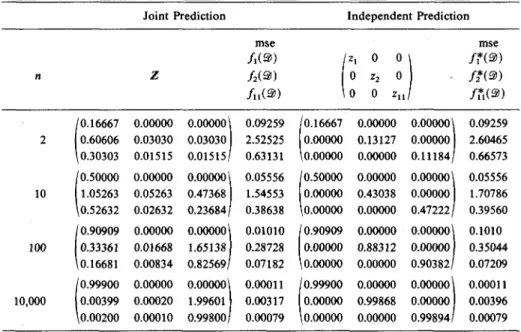
EXAMPLE C. Consider Example 3 from Section 3, the Poisson (TT), with Gamma prior, and hyperparameters: X01 = 10; nOi = 10. The marginal moments

are:

M = {1,2.1,1.1, 5.62,2.42,1.32,18.336,6.776, 5.456, 3.036,1.716}. The hyperparameters were again chosen to make m, = 1.0 and n0l = 10.0, but

now nO2= 12.31, and nou(n) = 10.43 + (4.35/(n-l)).

Figure 3 tabulates the results for n = 2, 10, 100, and 10,000 in the same format as previous examples. n 2 10 100 10,000 0.16667 0.60606 0.30303 0.50000 1.05263 0.52632 0.90909 0.33361 0.16681 0.99900 0.00399 0.00200 Joint Z 0.00000 0.03030 0.01515 0.00000 0.05263 0.02632 0.00000 0.01668 0.00834 0.00000 0.00020 0.00010 Prediction 0.00000 0.03030 0.01515 0.00000 0.47368 0.23684 0.00000 1.65138 0.82569/ 0.00000 1.99601 0.99800 mse /,(S>) /2O) fuiai) 0.09259 2.52525 0.63131 0.05556 1.54553 0.38638 0.01010 0.28728 0.07182 0.00011 0.00317 0.00079

1

0.16667 0.00000 0.00000 0.50000 0.00000 0.00000 0.90909 0.00000 0.00000 0.99900 0.00000 0.00000 Independent Prediction z, 0 0 0 z2 0 0 0 Zn 0.00000 0.13127 0.00000 0.00000 0.43038 0.00000 0.00000 0.88312 0.00000 0.00000 0.99868 0.00000 \ • / 0.00000 0.00000 0.11184 0.00000 0.00000 0.47222 0.00000 0.00000 0.90382/ 0.00000 0.00000 0.99894 mse /,*O) /*(2>) /?,(9) 0.09259 2.60465 0.66573 0.05556 1.70786 0.39560 0.1010 0.35044 0.07209 0.00011 0.00396 0.00079

FIGURE 2. Numerical results for Example B, Gamma-Exponential. We notice that:

(1) As in Example A and B, the first moment uses only fi(2>), but the second moments use all three statistics, with t2{3>) playing a decreasingly important role.

In contrast to Example B, however, we now find that, as n-»oo, fi(2)) + <n(20

is the preferred predictor for m2(2>), rather than t2(3>).

(2) This is a consequence of the assumption that the likelihood is Poisson, for then m2(d) = mx(d) + m\(6) for all 6, so that m2(®) = m1(2)) + mn(®) for any

prior. It is the assumption of the Gamma prior that makes predictions using only linear functions of t(3)) exact, and in fig. 3 we can see that, in fact, z2j = Zy + z3j

(j = 1,2,3), so that /2(9) =/1(®)+/u(@) for all 3)!

(3) The mse's follow the pattern of Example B, with the mse of/*(2>) becoming progressively relatively worse than its joint counterpart. Here, however, to improve the prediction error, one would probably have to include both tx{3>) and tu(3)),

n 2 10 100 10,000 0.16667 0.45833 0.29167 0.50000 1.02500 0.52500 0.90909 1.08264 0.17355 0.99900 1.00110 0.00210 Joint Z 0.00000 0.01389 0.01389 0.00000 0.02500 0.02500 0.00000 0.00826 0.00826 0.00000 0.00010 0.00010 Prediction 0.00000 0.01389 0.01389 0.00000 0.22500 0.22500 0.00000 0.81818 0.81818 0.00000 0.99790 0.99790/ mse

/.O)

/

2

O)

/11O) 0.08333 0.87472 0.42472 0.05000 0.52850 0.25850 0.00909 0.09691 0.04782 0.00010 0.00107 0.00053 / \ 0.16667 0.00000 0.00000 0.50000 0.00000 0.00000 0.90909 0.00000 0.00000 0.99900 0.00000 0.00000 Independent Prediction zi 0 0 0 z2 0 0 0 zu 0.00000 0.13973 0.00000 0.00000 0.44816 0.00000 0.00000 0.89036 0.00000 0.00000 0.99877 0.00000 0.00000 0.00000 0.11917 0.00000 0.00000 0.47806 0.00000 0.00000 0.90515 0.00000 0.00000 0.99896 mse

ma»

f*(3>) /,*,(2>) 0.08333 0.89985 0.44570 0.05000 0.57723 0.26410 0.00909 0.11468 0.04799 0.00010 0.00129 O.OOO53

FIGURE 3. Numerical results for Example C, Gamma-Poisson.

just t2{3>). Furthermore, neither of the other statistics would ever become "fully

credible" as n->oo, as they are not individually equal in expectation to m2, only

in sum. Clearly, the best single statistic to use for m2(2) in the Poisson case is

12. COMPUTATIONAL STRATEGIES; CONCLUSION

The last two examples show that some care must be exercised if one wishes to make independent forecasts where p{x\6) is assumed-to be in the QVF-NEF family, remembering that this also includes (fixed numbers of) convolutions of Examples 1-6, such as the Negative Binomial with fixed shape parameter. One can, of course, use the combination of "natural" statistics appropriate to the assumed likelihood. This is particularly important when we also assume that the natural conjugate prior is appropriate.

On the other hand, for an arbitrary prior, the moments will not be linear functions of the statistics, so that all positions of Z would be non-zero anyway, as would also be the case if all moments were from empirical studies. In these cases, Z would approach the identity matrix as n-»oo, and we expect that the independent forecasts (2.2), (6.1), (6.2) would be equally good (or equally bad) as the joint forecasts. Clearly, more computational experience is needed in making this decision.

The great advantage of the joint forecast is that it can always be used if n ^ 2, and, if there is a tendency for certain combinations of statistics to dominate, it

will be revealed automatically. Of course, if n = 1, we are forced to use only ti(2fi) = xl and t2(2)) = xl; the predictive power will be weak anyway, in most

practical cases.

In summary, we have presented an easily implemented three-dimensional credibility formula that simultaneously approximates the first and second moments of the Bayesian predictive density. While this approach requires eleven prior moments from the collective, this calculation is simplified when familiar analytic forms are assumed for the likelihood. Previous work has shown that the credibility mean is exact in tx(3>) for a wide class of likelihoods and priors in

which the sample mean is the sufficient statistic; here we have shown that the second-moment credibility predictions are also exact for five widely-used likeli-hoods and their natural conjugate priors, when using the three "natural" statistics in t(3)).

For these and other reasons, we believe that these linear prediction formulae will turn out to be robust in other cases where the distributions are empirical, or where the exact predictions are known to be non-linear in the data. We suspect also that, in most cases, it will also be reasonable to use the simplified, independent forecasts, paying due attention to the remarks above. The authors look forward to hearing from those who apply this approach to actual prediction problems.

REFERENCES

BUHLMANN, H. (1967) Experience Rating and Credibility. Astin Bulletin 4, 199-207. BOHLMANN, H. (1970) Mathematical Methods in Risk Theory. Springer-Verlag: New York. GERBER, H. (1980) Introduction to the Mathematical Theory of Risk, The Huebner Foundation,

Philadelphia, PA.

HACHEMEISTER, C. A. (1974) Credibility for Regression Models with Application to Trend. In Credibility Theory and Applications, P. M. Kahn (ed.), Academic Press: New York.

JEWELL, W. S. (1974a) Credible Means are Exact Bayesian for Simple Exponential Families. Astin

Bulletin 7, 237-269.

JEWELL, W. S. (1974fc) Exact Multidimensional Credibility. Mitteilungen der Vereinigung

schweizeris-cher Versischweizeris-cherungsmathematiker 74, 193-214.

JEWELL, W. S. (1975) Regularity Conditions for Exact Credibility. Astin Bulletin 8, 336-341. JEWELL, W. S. (1980) Models in Insurance: Paradigms, Puzzles, Communications, and Revolutions.

Transactions 21st International Congress of Actuaries, Zurich and Lausanne, Volume S, 87-141.

JEWELL, W. S. (1983) Enriched Multinomial Priors Revisited. Journal of Econometrics 23, 5-35. MORRIS, C. N. (1982) Natural Exponential Families with Quadratic Variance Functions. The Annals

of Statistics 10, 65-80.

NORBERG, R. (1979) The Credibility Approach to Experience Rating. Scandinavian Actuarial Journal, 181-221.