HAL Id: hal-02925913
https://hal.inria.fr/hal-02925913
Submitted on 31 Aug 2020
HAL is a multi-disciplinary open access
archive for the deposit and dissemination of
sci-entific research documents, whether they are
pub-lished or not. The documents may come from
teaching and research institutions in France or
L’archive ouverte pluridisciplinaire HAL, est
destinée au dépôt et à la diffusion de documents
scientifiques de niveau recherche, publiés ou non,
émanant des établissements d’enseignement et de
recherche français ou étrangers, des laboratoires
A Unified Framework for Multimodal Structure-function
Mapping Based on Eigenmodes
Samuel Deslauriers-Gauthier, Mauro Zucchelli, Matteo Frigo, Rachid Deriche
To cite this version:
Samuel Deslauriers-Gauthier, Mauro Zucchelli, Matteo Frigo, Rachid Deriche. A Unified Framework
for Multimodal Structure-function Mapping Based on Eigenmodes. Medical Image Analysis, Elsevier,
2020, pp.22. �10.1016/j.media.2020.101799�. �hal-02925913�
A Unified Framework for Multimodal Structure–function
Mapping Based on Eigenmodes
Samuel Deslauriers-Gauthier, Mauro Zucchelli, Matteo Frigo, and Rachid Deriche
Inria Sophia Antipolis - Méditerranée, Université Côte d’Azur, France
Abstract
Characterizing the connection between brain structure and brain function is essential for understanding how behaviour emerges from the underlying anatomy. A number of studies have shown that the network structure of the white matter shapes functional connectivity. Therefore, it should be possible to predict, at least partially, functional connectivity given the structural network. Many structure–function mappings have been proposed in the literature, including several direct mappings between the structural and functional connectivity matrices. However, the current literature is fragmented and does not provide a uniform treatment of current methods based on eigendecompositions. In particular, existing methods have never been compared to each other and their relationship explicitly derived in the context of brain structure–function mapping. In this work, we propose a unified computational framework that generalizes recently proposed structure–function mappings based on eigenmodes. Using this unified framework, we highlight the link between existing models and show how they can be obtained by specific choices of the parameters of our framework. By applying our framework to 50 subjects of the Human Connectome Project, we reproduce 6 recently published results, devise two new models and provide a direct comparison between all mappings. Finally, we show that a glass ceiling on the performance of mappings based on eigenmodes seems to be reached and conclude with possible approaches to break this performance limit.
1
Introduction
Characterizing the connection between brain structure and brain function is essential for under-standing how behaviour emerges from the underlying anatomy (Sporns et al.,2005). To this end, a common representation of the brain is that of a network or graph, where nodes represent cortical and sub–cortical gray matter volumes and edges represent the strength of structural or functional
connectivity (Rubinov and Sporns, 2010; Sporns, 2012; Chu et al., 2018). Typically, the struc-tural network is constructed from a set of streamlines obtained from diffusion magnetic resonance imaging (MRI) tractography. The functional network is constructed by correlating the functional MRI blood oxygenation level–dependent (BOLD) signal of cortical regions under the assumption that strong correlation reflects connectivity. Together, the structural and functional networks, also referred to as the structural and functional connectomes, provide two different points of view on brain connectivity.
A number of studies have shown that the network structure of the white matter shapes func-tional connectivity (Honey et al., 2007,2010;Skudlarsky et al., 2008;Atasoy et al., 2016). While the relationship is not local or one to one (Mišić et al., 2016), structural and functional connec-tomes are related by analytical operations (Saggio et al., 2016) and simple linear models may be sufficient to characterize resting state dynamics (Deco et al.,2013). The joint analysis of structure and function has also been considered to identify function–specific brain circuits (Chu et al.,2018) or map information flow in the white matter (Deslauriers-Gauthier et al.,2019). All of these re-sults support the hypothesis that the structural network acts as a substrate on which functional connectivity emerges (Honey et al., 2007, 2010). Therefore, it should be possible to predict, at least partially, functional connectivity given the structural network. More specifically, generative models making use of the structural network should be able to predict functional connectivity more reliably than those that do not (Goñi et al.,2012). Many structure–function mappings have been proposed in the literature which can broadly be separated into two classes. The first class relies on generative models of functional activity with various degrees of complexity (Galán, 2008; Honey et al., 2009;Deco et al.,2011; Deco and Jirsa, 2012;Messé et al., 2015b,a). The output of these models is a simulated functional time–series with realistic dynamical properties whose correlation predicts the functional connectome. The second class relies on a more direct relationship between the structural and functional connectivity matrices (Deligianni et al.,2013;Abdelnour et al.,2014, 2018; Meier et al., 2016; Liang and Wang, 2017; Becker et al., 2018). These models attempt to predict the functional connectivity matrix from the structural connectivity matrix directly, with-out generating the intermediate functional time–series. A subset of these models rely specifically on the link between the eigenvalues and eigenvectors of the structural and functional connectivity matrices. The appeal of these so called eigenmode mappings lies in their high prediction accuracy despite their relative simplicity, in particular when compared to sophisticated generative models of brain activity. Furthermore, certain eigenmode mappings are invertible, allowing structure to be predicted from function. Although mapping strategies of this class share a modus operandi, the current literature is fragmented and does not provide a uniform treatment of current methods.
Abdelnour et al.(2018) notes that diffusion processes on a graph, random walks, and eigenmode decompositions which underly the current models are known to be closely linked, however they do not explore this relationship further. More generally, existing methods have never been compared to each other and their relationship explicitly derived in the context of brain structure–function mapping. There is therefore a need for a unified treatment of structure–function mapping based on eigenmodes.
In this work, we show that current mappings based on eigenmodes are strongly related and that they can be unified by a more general model. Using this generalized approach, we are able to reproduce previously published results and devise new models whose performance is also tested. Finally, we show that a glass ceiling on the performance of mapping based on eigenmodes seems to be reached and conclude with possible approaches to break this performance limit.
2
Theory
Let SymN denote the space of N × N real symmetric matrices and let Sk ∈ SymN and Fk∈ SymN
be the structural and functional connectivity matrices of subject k, respectively. The size of the matrices N corresponds to the number of regions of the atlas. The entry (i, j) of these matrices quantifies the strength of the connectivity between regions i and j evaluated either functionally or structurally. To simplify the notation, the subject subscript will be dropped if the discussion involves a single subject. The objective of structure–function mapping is to identify a mapping f : SymN → SymN such that f (Sk) = Fk. Two types of structure function mapping strategies can
be distinguished. The first involves finding multiple mappings from the structure to the function of individual subjects. Given K subjects, the identification can be formulated as K independent optimization problems of the form
minimize
fk
kfk(Sk) − Fkk2F (1)
for k = 1 . . . K where k · kF is the Frobenius norm and where fk is the mapping of subject k. The
result of this strategy is a set of K subject specific mappings. Because the mapping fk is subject
specific, learning its parameters requires at least one pair of structure and function matrices for each subject. Once learned, it can be used to predict functional changes resulting from a structural change in a subject specific manner. We refer to this strategy as single–subject.
The second strategy involves finding a unique mapping from the structure to the function of all subjects simultaneously. This problem can be formulated as
minimize f K X k=1 kf (Sk) − Fkk2F (2)
where f is a global mapping. Because the learned mapping f is global, it allows the functional connectivity matrix to be predicted for any subject, given his structural connectivity matrix. In theory, this mapping could allow to study functional changes in a population without acquiring any functional data, provided that structural data is available. In addition, if the mapping f can be inverted, it may also allow the prediction of the structural connectivity matrix from the functional connectivity matrix.
Let {(Sk, Fk)} with k = 1, . . . , K + T be a set of pairs of structural and functional matrices.
The first K matrices are used to learn the parameters of the mapping from one of the optimization problems above. The remaining T matrices are used to evaluate the performance of the mapping. Previously published literature used the correlation between the predicted and observed functional connectomes on the testing set, ρk = corr(f (Sk), Fk) with k = K +1, . . . , T , as an absolute measure
of performance. While different definitions of the correlation were used across publications, here we compute the more common Pearson correlation, using the lower triangular part of the matrices and excluding the main diagonal. We therefore have
corr(A, B) = PN −1
i=1
Pi−1
j=0(Aij− ¯A)(Bij− ¯B)
kAkSymNkBkSymN
where the symmetric matrix norm and the overbar are defined as
kXkSymN = N −1 X i=1 i−1 X j=0 (Xij− ¯X)2 and ¯X = 2 N2− N N −1 X i=1 i−1 X j=0 Xij.
While it is undoubtedly true that maximizing the correlation is desirable, this evaluation strategy does not provide a minimum performance at which mappings become relevant. To define this minimum requirement, we return to the objective of structure–mapping. Given a training set of structure and function matrices and a new structure matrix, can we predict the function associated with this new matrix? If structure does indeed support function, mappings making use of the structural information should outperform those that do not. A straightforward way to predict the functional connectomes of the testing set is simply to use the mean functional matrix of the training set. In the specific case where the variance of the functional connectivity cannot be explained by the variance of the structural connectivity, this zeroth order estimator would in fact be optimal. We can therefore introduce a reference mapping defined as
fref(S) = 1 K K X k=1 Fk= ¯F (3)
for k = 1, . . . , K. This mapping always returns the average functional connectivity matrix of the training set, independently of the structural matrix received. Any mapping that makes use of the structural information to predict subject specific functional variance should outperform this
reference mapping. In other words, mappings should capture the subject specific variance of the functional connectivity and not only its mean.
2.1
Structure–function mappings
Abdelnour et al.(2014,2018) model the functional connectivity matrix as the result of a diffusion process on the graph defined by the structural connectivity. Let L = ∇2S = I − D−1/2SD−1/2
where D is a diagonal matrix with entries Dii = PjSij be the normalized Laplacian of the
structural adjacency matrix as defined inAbdelnour et al.(2014). The structure function mapping proposed byAbdelnour et al. is then given by
f (L) = e−βLt (4) in their early work and by
f (L) = ae−αL+ bI (5) in the latter with I the identity matrix. In terms of number of degrees of freedom, these two models are the sparsest, having only 1 and 3 parameters, respectively. In addition to an explicit mapping from structure to function, the graph Laplacian has also been used as a basis for the resting state networks byAtasoy et al.(2016). Although they do not explicitly derive a structure to function mapping, their results do highlight a relationship between eigenfunctions of the graph Laplacian and resting state networks. Meier et al.(2016) propose to model functional connectivity matrices as a weighted sum of powers of structural connectivity matrices, that is
f (S) =
M
X
m=0
amSm (6)
where am∈ R are the weights. The value of M, which sets the number of parameters of the model
to M + 1, is empirically selected and typically close to 10. The rational is that the mth power of
the structural connectivity matrix represents the influence on a node of the nodes m steps away. Liang and Wang(2017) use a more general version of the same mapping with the addition of a constant which represents global input
f (S) =
M
X
m=0
amSm+ C (7)
with C ∈ SymN. This addition of the constant significantly increases the complexity of the model
by adding (N2+N )/2 parameters. Becker et al.(2018) also proposed a spectral mapping approach,
but included the notion of rotation of eigenvectors. Their suggested structure to function mapping is given by f (S) = R M X m=0 amSm ! RT (8)
where R is a rotation matrix, meaning RRT = RTR = I. This additional rotation matrix adds (N2− N )/2 parameters to the mapping. While the mapping of Eq. (8) can be used in the multi– subject case, it was only used byBecker et al.(2018) to generate individual subject mappings. For multi–subject mapping, they instead suggest to use
f (S) = Q M X m=0 amΣm ! QT (9)
where S = U ΣUT is the singular value decomposition of S. The difference between the two models is that Eq. (8) allows for subject specific functional eigenvectors given by RUk, whereas
the model in Eq. (9) assumes all subjects share the same functional eigenvectors Q. The subject specific variance is therefore obtained only by mapping the eigenvalues. Like the rotation matrix, this change adds (N2− N )/2 degrees of freedom to the model.
2.2
Relationship between mappings
In an effort to provide a uniform view of structure–function mapping based on eigenmodes, we start by highlighting the relationship between the mappings described in the previous section. First, let us start with the single subject model proposed byBecker et al.(2018) in Eq. (8), which can be rewritten as f (S) = RU M X m=0 amΣm ! UTRT = N −1 X n=0 M X m=0 amσmn ! RunuTnR T = N −1 X n=0 g(σn)h(un)
where N is the size of S and corresponds to the number of brain regions, and σnare the eigenvalues
of S. This mapping can therefore be factorized into a mapping on the eigenvalues, here a polynomial regression of degree M , g(λn) = M X m=0 amσmn (10)
and a mapping on the eigenvectors
h(un) = RunuTnR T.
Factorizing the multi–subject mapping of Eq. (9) yields the same g, but a different eigenvector mapping h(un) = qnqTn where qn is the nth column of Q. Again, this result highlights that under
only by mapping the eigenvalues. Similar results are obtained for the spectral mapping of Eq. (6) since we can set R = I yielding h(un) = unuTn. Finally, the mapping of Eq. (7) simply requires
an addional constant C.
Now let us consider the mapping ofAbdelnour et al.(2014) in Eq. (4). It can be rewritten as f (L) = e−βLt= V e−βΛtVT = N −1 X n=0 e−βλntv nvnT
where L = V ΛVT is the eigendecomposition of L, and vnand λnare eigenvectors and eigenvalues
of the Laplacian, respectively. Again we obtain two mappings, one on the eigenvectors g(λn) =
e−βλntand one on the eigenvectors h(v
n) = vnvnT. Further expanding g using the Taylor series of
the exponential yields
g(λn) = ∞ X m=0 (−βt)m m! λ k n.
Comparing with the eigenvalue mapping of Becker et al. (2018) in Eq. (10) we can see that the exponential decay is a special case where
am=
(−βt)m m!
and the truncated sum is extended to infinity. Finally, similar results are obtained using the same approach on the model ofAbdelnour et al.(2018) in Eq. (5) with the weights given by
a0= a + b and am=
a(−α)m
m! for m > 0.
From these results, it should be clear that the graph diffusion based approaches ofAbdelnour et al.(2014,2018) are particular cases of the more general graph spectral mapping. Surprisingly, while the two approaches can be reformulated to a common framework, the matrix supplied as input to f is different. On one hand, spectral mapping use the structural connectivity matrix as input while graph diffusion use its Laplacian. In addition, graph diffusion assumes the eigenvectors of the graph Laplacian correspond to those of the functional connectivity matrix. This allows the eigenvectors of the Laplacian to be used with no further transformation as estimators of those of the function connectivity matrix, which are not known a priori. Conversely, spectral mapping assumes the eigenvectors of the structural connectivity matrix, and not those of it’s Laplacian, directly correspond to the eigenvectors of the functional connectivity matrix. One exception is the model of Becker et al. (2018) which assumed they must be rotated by R to obtain those of the output.
2.3
General form
The relationship between the structure–function mapping presented in the previous section hints at a unified framework. Let the map f have the form
f (A) =
N −1
X
n=0
g(λn)h(un) + C (11)
where C ∈ SymN is a constant and where λn ∈ R and un ∈ RN are the nth eigenvalue and
eigenvector of A ∈ SymN, respectively. The function h : RN → Sym
N is a mapping from an
eigen-vector to an eigenmode1
and g : R → R is the associated weighting. By selecting the appropriate definition of g, h and C, Eq. (11) can be simplified to the previously published mappings. The specific definitions to use are specified in Table 1 and include the number of degrees of freedom of each model. For example, to obtain the mean mapping introduced in Section 2, C can be set to the mean functional connectivity matrix of the training set ¯F and g and h always return zero (mapping 0 of Table1). In addition to reproducing existing mappings, the general form can be used to generate new mappings by combining the features of existing ones. For example, the models proposed byBecker et al.(2018) (mappings 6 and 7 of Table1) can be modified to add the mean of the functional matrices in the constant C, borrowed from the work ofLiang and Wang (2017). This results in two new mappings that capture the inter–subject functional connectivity variance instead of the mean.
Depending on the selected values of g, h, and C, minimizing equations (1) or (2) may be challenging because the objective function is non–linear and non–convex. We used an iterative procedure, as in Becker et al. (2018), where the only parameters of g, h, or C are allowed to vary in turn. The full optimization procedure therefore iterates over three subproblems. For the minimization of over the parameters h, Pymanopt (Townsend et al.,2016) was used to ensure that R is a rotation matrix and that Q is orthonormal, respectively. Pymanopt was also used when minimizing over C to ensure it is a symmetric matrix. Additional information on the optimization procedure is provided in the supplementary materials.
2.4
Evaluation
The performance of the mappings described in Table1 are evaluated by quantifying their ability to predict a subject’s functional connectivity matrix given his structural connectivity matrix. For the individual mapping, the parameters of the subject specific mappings are learned using the first resting state session and evaluated on the second resting state session. For the global mapping, a
1Here, we use the term eigenmode to refer to the outer product of an eigenvector with itself. An eigenmode is therefore a symmetric rank 1 matrix derived from an eigenvector.
Mapping Reference A g(λ) h(un) C DOF 0 S 0 0 F¯ (N2+ N )/2 1 S λ unuTn 0 0 2 Abdelnour et al.(2014) ∇2S e−βtλ u nuTn 0 1 3 Abdelnour et al.(2018) ∇2S ae−αλ u nuTn bI 3 4 Meier et al.(2016) S PM m=0amλm unuTn 0 M + 1
5 Liang and Wang(2017) S PM
m=0amλm unuTn C M + 1 + (N2+ N )/2 6 Becker et al.(2018) S PM m=0amλm RunuTnRT 0 M + 1 + (N2− N )/2 7 Becker et al.(2018) S PM m=0amλ m q nqTn 0 M + 1 + (N2− N )/2 8 S PM m=0amλm RunuTnRT F¯ M + 1 + N2 9 S PM m=0amλm qnqTn F¯ M + 1 + N 2
Table 1: Definitions used in the general form to obtain the previously published models and new ones. S is the structural matrix, ∇2S is the Laplacian of the structural matrix, λ is an eigenvalue, 0 is an N × N matrix of zeros, un is the nth eigenvector, C is a symmetric N × N matrix, and
¯
F is the average functional connectivity matrix of the training set. When the parameters yield a previously published mapping, the corresponding reference is indicated. The number of degrees of freedom (DOF) of each model is also provided in the last column.
leave-one-out cross-validation strategy was used. Specifically, the parameters of the mapping are learned by minimizing Eq. (2) while leaving a single subject out. The mapping is then evaluated on the left out subject and the process is repeated for all subjects. In all cases, the mapping per-formance is evaluated by computing the mean and standard deviation of the normalized prediction error given by the functional
E(f ) = kf (S) − F k 2 F kF k2 F . (12)
3
Methods
3.1
Data and data processing
The data was provided by the Human Connectome Project2 (HCP) and our processing started
from the minimally processed data (Glasser et al., 2013) for both diffusion and functional MRI data. For 50 randomly selected subjects, the brain was extracted using FSL bet (Smith, 2002) and the white matter, gray matter, and cerebrospinal fluid were segmented using FSL fast (Zhang et al.,2001). Using the FreeSurfer3segmentation (Fischl,2012) and the diffusion weighted images,
a single fiber response function was computed for the white matter, gray matter, and cerebrospinal fluid using MRtrix34(Tournier et al.,2019). These response function were then used to compute
a fiber orientation distribution function for each voxel using contrained spherical deconvolution (Tournier et al., 2007). Two million streamlines were generated using anatomically constrained probabilistic tractography using a step of 0.3 mm, a maximum length of 300 mm, and backtracking (Smith et al., 2012). In an effort to make connectomes more quantitative and to reduce the impact of false positive connections (Maier-Hein et al., 2017) by re-establishing the biological interpretability of streamline-based structural connections, the tractograms were filtered using SIFT2 (Smith et al., 2015) assigning a weight to each streamline representing its cross-sectional area. The cortical surface extracted with FreeSurfer was parcellated using the Desikan–Killiany atlas into N = 68 regions. Given the parcellation and the streamlines, a first structural connectome was built by counting the number of streamlines connecting all pairs of cortical regions while ignoring self connections. A second connectome was built by summing the SIFT2 weights of streamlines connecting two cortical regions and a third by using the reciprocal average length of the streamlines connecting two regions. These three connectomes are identified as the count, SIFT2, and length connectomes respectively. In all cases, the connectomes were symmetrized by summing the (i, j) and (j, i) entries of the connectome. Finally, the structural connectomes were normalized by dividing by the sum of the off diagonal entries. While some authors removed weak connections we followed the recommendations of Civier et al. (2019) and omitted pruning thus keeping weak connections. The rational is that weak connections have little impact on values derived from connecivity matrices. It is therefore preferable to simplify the processing pipeline and reduce the number of arbitrary parameters by omitting this step.
The resting state functional MRI data provided by the HCP offfers two sessions each containing two acquisitions, one with left to right encoding and one with right to left encoding. Here, we made
2https://www.humanconnectome.org 3https://surfer.nmr.mgh.harvard.edu/ 4http://www.mrtrix.org
use of the first (REST1) session and preprocessed the two acquisitions as follows. The time series were filtered using a butterworth bandpass filter with critical frequencies 0.01 and 0.1 Hz. The first 20 volumes of each acquisition were dropped and the remaining volumes linearly detrended. The movement parameters and their derivatives were regressed out and the data was motion scrubbed (Power et al., 2012). After this preprocessing, we concatenated both acquisitions to produce a single dataset per subject. The mean signal for each parcel was computed and used to build the functional connectivity matrix using Pearson correlation. Finally all negative entries of the matrix, corresponding to anticorrelations between cortical regions, were set to zero.
4
Results
4.1
Direct structure–function correlation
First, we compute the Pearson correlation of structural and functional connectivity matrices across all subjects. The structural connectivity matrices are highly correlated across subjects with a mean correlation of 0.91, 0.88, and 0.92 for the counting, length, and SIFT2 connectomes respectively. On the other hand, functional connectivity matrices obtained a correlation of 0.61. The functional matrices are poorly correlated with structural matrices both across and intra–subject with a mean correlation of 0.25, 0.29, and 0.24 for the count, length and SIFT2 matrices, respectively. These correlations are illustrated in Figure1. The banded nature of the structure function correlation present across all three matrices can be explained by noting the very strong correlation of structural matrices. Indeed, if a functional connectivity matrix is correlated with one structural connectivity matrix, it is correlated with all of the them. The absence of a diagonal in the structure function correlation is also notable. It suggests that the functional matrix of a subject is not more correlated with his own structural matrix than with the structural matrix of another subject.
4.2
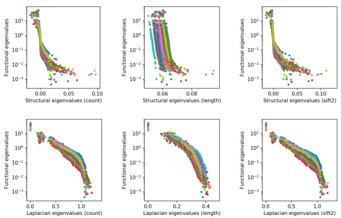
Eigenvalue mapping
Figure2illustrates the normalized eigenvalues of the functional connectivity matrix as a function of the eigenvalues of the structural or Laplacian of structural connectivity matrix. A strong log-linear relationship can be observed between the eigenvalues of the length structural connectivity matrix and the eigenvalues of the functional connectivity matrix (top middle pane). However, unlike the results reported byAbdelnour et al. (2018), we did not observe a log-linear relationship over all eigenvalues of the Laplacian of the count structural connectivity matrix and the eigenvalues of the functional connectivity matrix (bottom left pane). Instead, we found a piecewise log-linear relationship with a transition at eigenvalues near 1. A possible explanation for this discrepancy
Figure 1: Illustration of the inter–subject correlation between the functional connectivity matrix and the count (a), length (b), and SIFT2 (c) matrices.
is the differences in the processing pipeline; we used a fiber orientation distribution based proba-bilistic tractography algorithm whereas they relied on a tensor based deterministic approach. By comparing the panes of the first and last columns, we also observe that the SIFT2 filtering does not significantly change the relationship between structural and functional eigenvalues.
4.3
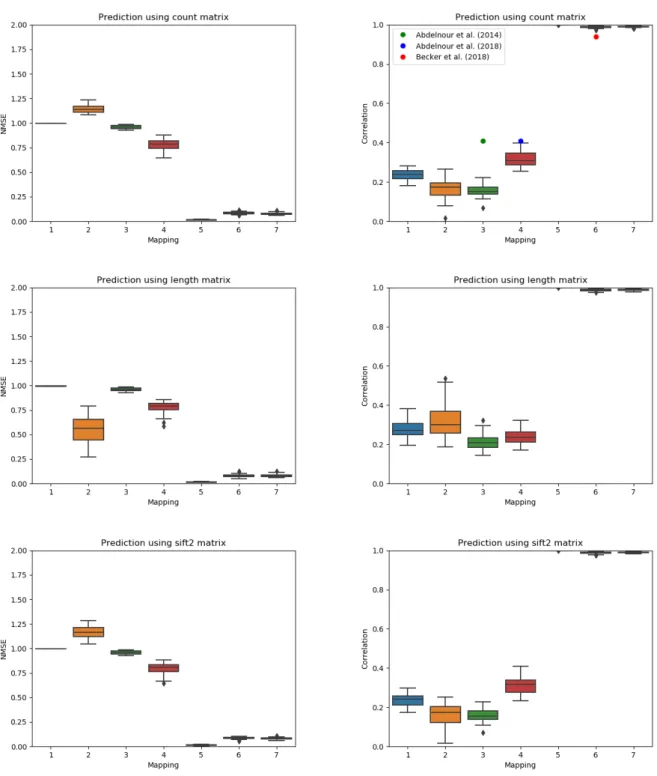
Structure–function mapping
Figure 3 illustrates the NMSE and correlation for the single–subject stategy of Eq. (1). The mappings of Table1 involving the mean ¯F are omitted because only a single functional matrix is available for this strategy. The mapping ofLiang and Wang(2017) obtains the best performance with a correlation very close to 1. However, it should be noted that this is achieved by setting the constant C to the functional matrix of the training and leaving the other parameters of the model at 0. The other spectral mapping approaches that optimized over the eigenvectors (mappings 5, 6 and 7) also performed well, obtaining a correlation above 0.98. On the other hand, the graph diffusion based mappings and the spectral mapping which fixes the eigenvectors (model 2) obtained a correlation between 0.15 and 0.40. Figure 3 also illustrates the correlations reported byAbdelnour et al.(2014,2018);Becker et al.(2018);Liang and Wang(2017) using colored dots. Despite differences in the data and processing pipeline, the reported correlations generally agree with those obtained using our unified framework.
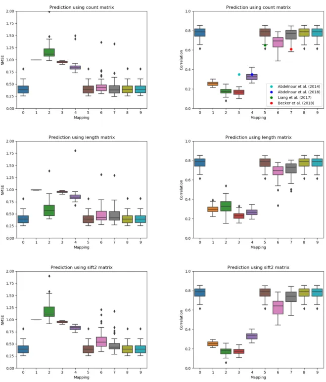
Figure4illustrates the multi–subject NMSE and correlation of each model described in Table1 and for each structural matrix type. Mapping 0, which simply estimates the mean functional con-nectivity, obtains a correlation value of 0.77 regardless of the structural input since it is ignored.
Figure 2: Functional eigenvalues as a function of the structural and Laplacian eigenvalues. Each dot correponds to one eigenvalue pair with the colors corresponding to subjects. The top row relates the eigenvalues of the functional connectivity matrix directly to those of the structural connectivity matrix whereas the bottom row relates them to the eigenvalues of the Laplacian of the structural connectivity matrix. Note the use of a logarithmic scale for the ordinates.
Mapping 1, the identity mapping, which corresponds to a direct correlation between structure and function, obtains a mean correlation of 0.25, 0.30, and 0.25 for the count, length, and SIFT2 matrices, respectively. Mappings 2, 3, and 4, which all assume the eigenvectors of the functional connectivity matrix are those of the structural connectivity matrix (or its Laplacian), obtain a cor-relation between 0.17 and 0.33. Their performance therefore relies mostly on the correct mapping of the eigenvalues. Mapping 5, which correponds to a spectral mapping with a constant, obtained a correlation of 0.75. Mapping 6, which was proposed by Becker et al.(2018), but only used for single subject mapping in their work, obtains a correlation close to 0.65 for all input types. The multi–subject version (model 7) obtains a higher correlation, reaching 0.75 when using the count matrix as input. Finally, the two new models which include the mean functional matrix as a con-stant obtain a performance of 0.77, the same as model 0. The correlations reported byAbdelnour et al.(2018);Becker et al.(2018);Liang and Wang(2017), which all rely on the count matrix, are
illustrated using colored dots. Despite differences in the data and processing pipeline, the reported correlations generally agree with those obtained using our unified framework.
5
Discussion
Understanding the relationship between brain structure and function is a fundamental problem of neuroscience. Many studies have shown that the structural substrate drives functional activity, yielding the idea that it may be possible to predict the functional connectome from the structural connectome. In this work, we investigated structure–function mappings based on eigenmodes and showed that current models can be generalised and unified in a single framework. We used this framework to reproduce previously published results and, for the first time, directly compare the different mappings against each other.
First, by using our general model, we were able to reproduce previously published results obtained by specific models. In addition to the intrinsic value of reproducibility, this highlights the robustness of the results to changes in the processing pipeline. When mapping structure to function, the model does not only capture the relationship between structure and function, but also how they were measured. The processing pipelines used could therefore be expected to have an impact on the performance of the mappings. While evaluating the plethora of possible diffusion MRI and functional MRI pipeline variations is out of the scope of the current work, some predictions can be made on the basis of our results. Indeed, the tractography and functional MRI processing pipeline used in this study differed from the ones used inAbdelnour et al.(2014,2018); Meier et al. (2016); Becker et al. (2018). Notable differences included the use of probabilistic tractography rather than deterministic, the addition of the SIFT2 filtering, and the use of different brain parcellations. Based on our ability to reproduce the performance of different models, we believe that these choices do not significantly change the performance of the mappings.
In addition to simplifying to the previous models, our generalized approach allowed us to combine the features of the different models to produce new ones. This allowed us to test new models, which obtained state of the art performance. Interestingly, none of the tested models were able to outperform the mean mapping which does not make use of the structural information. One possible explanation for this apparent glass ceiling is the very high correlation (0.91) of the structural connectomes. All mappings attempt to explain subject specific variations in functional connectivity using variations in structural connectivity. However, if all structural connectomes are very similar, or identical in the limiting case, no variation can be leveraged and the best estimator is a simple mean. Thus, for very homogeneous cohorts such as the one used in this study, inter
subject structural variations may not be sufficient to overcome the noise added by the imaging and processing pipelines. As a preliminary test to verify this hypothesis, an additional experiment was performed. Functional connectivity matrices were simulated by using mapping 8 from Table1 with fixed parameters trained using the data of this study. Structural connectivity matrices with their entries randomly permuted were used as input to produce new structure–function pairs. This results in a dataset with poorly correlated structural matrices, but with a structure–function relationship perfectly matched to the mapping. On this test data, the mean (mapping 0) obtained a mean correlation of 0.58 and mappings 6 and 8 obtained a correlation of 0.76 and 0.93. The other mappings obtained a correlation below 0.4. Therefore, on less homogenious data, mappings based on eigenmodes do indeed provide additional information not captured by the mean. These findings are particularly interesting in the case of pathology, where specific connections or subnetworks may be perturbed. The variance in structural connectivity across patients and controls may lead to improved performance of mappings based on eigenmodes. Another potential application is the prediction of brain states following perturbations to the structural connectome (Deco et al.,2019). In this work, we focused on the ability of mappings based on eigenmodes to predict the complete functional connecvity matrices from the full structural connectivity matrix. However, recent work has shown that certain subnetworks way be more strongly associated with function than others (Medaglia et al.,2018;Preti and Van De Ville,2019). It may therefore be interesting to investigate how the mappings reviewed here are able to predict the functional connectivity matrix using only a subset of the structural connectivity matrix. In this case, the full functional connectivity matrix would be predicted by a combination of mappings, each operating on a subnetwork of the full structural connectome.
It is important to note that all models reviewed here operate on a very high level to predict the function given the structure, and make no attempt at realistic biophysical modeling. In addition, the values of the parameters obtained after fitting are never interpreted or tested for significance. As a consequece, while the models do have a varying number of parameters, identifying the most efficient model, in the sense of prediction performance per degrees of freedom, is not as critical as in other applications. The only objective of these mappings is the prediction of function from structure and any increase in complexity or additional parameters can be justified post hoc by an increase in performance.
Most of the litterature on structure–function mapping makes use of streamline count as an in-dication of structural connectivity strength. However, it is known that streamline count is biased towards large anatomical structures, making its correlation with connection strength uncertain. For this reason, we investigated the length and SIFT2 connectivity matrices in addition to the
count matrices as inputs to predict function. Despite their more quantitative nature, the predic-tions made using the length and SIFT2 matrices were very similar to those using the count matrix. Finally, we also considered a count connectome whose entries are normalized by the sum of the area of the cortical regions corresponding to each row and column. The rationale for this new con-nectome is that considering a density, rather than an absolute count, may reduce the bias towards large structures. The NMSE and correlation results for this density connectome (available in the supplementary materials) follow the same trends as the other three considered here, indicating that this normalization does not overcome the limitations of streamline counting.
6
Conclusion
In this work, we proposed a unified computational framework of structure–function mapping based on eigenmodes that allowed us to reproduce 6 recently published results, devise two new mappings, and provide a direct comparison between recently proposed mappings. Using this unified frame-work, we highlighted the link between existing mappings and showed how they can be obtained as particular cases of our framework. For individual mappings, our results highlighted the importance of mapping the eigenvectors and not only the eigenvalues, while for multi–subject mappings, our re-sults showed that a glass ceiling on the performance of mappings based on eigenmodes is reached, very likely because of the homogenous nature and the highly correlated structural connectivity matrices of our 50 subjects of the Human Connectome Project.
7
Acknowledgements
This work has received funding from the European Research Council (ERC) under the Euro-pean Union’s Horizon 2020 research and innovation program (ERC Advanced Grant agreement No 694665 : CoBCoM - Computational Brain Connectivity Mapping).
Data were provided by the Human Connectome Project, WU-Minn Consortium (Principal In-vestigators: David Van Essen and Kamil Ugurbil; 1U54MH091657) funded by the 16 NIH Institutes and Centers that support the NIH Blueprint for Neuroscience Research; and by the McDonnell Center for Systems Neuroscience at Washington University.
References
F. Abdelnour, H. U. Voss, and A. Raj. Network diffusion accurately models the relationship between structural and functional brain connectivity networks. NeuroImage, 90:335–347, 2014.
F. Abdelnour, M. Dayan, O. Devinsky, T. Thesen, and A. Raj. Functional brain connectivity is predictable from anatomic network’s Laplacian eigen-structure. NeuroImage, 172:728–739, 2018. S. Atasoy, I. Donnelly, and J. Pearson. Human brain networks function in connectome specific
hamonic waves. Nature Communications, pages 1–10, 2016.
C. O. Becker, S. Pequito, G. J. Pappas, M. B. Miller, S. T. Grafton, D. S. Bassett, and V. M. Preciado. Spectral mapping of brain functional connectivity from diffusion imaging. Scientific Reports, 8(1411), 2018.
S. H. Chu, K. K. Parhi, and C. Lenglet. Function–specific and enhanced brain structural connec-tivity mapping via joint modeling of diffusion and functional MRI. Scientific Reports, 8(4741), 2018.
O. Civier, R. E. Smith, C. H. Yeh, A. Connelly, and F. Calamante. Is removal of weak connections necessary for graph-theoretical analysis of dense weighted structural connectomes from diffusion MRI? NeuroImage, 194:68–81, 2019.
G. Deco and V. K. Jirsa. Ongoing cortical activity at rest: Criticality, Multistability, and Ghost Attractors. The Journal of Neuroscience, 32(10):3366–3375, 2012.
G. Deco, V. K. Jirsa, and A. R. McIntosh. Emerging concepts for the dynamical organization of resting–state activity in the brain. Nature Review Neuroscience, 12:43–56, 2011.
G. Deco, A. Ponce-Alvarez, D. Mantini, G. L. Romani, P. Hagmann, and M. Corbetta. Resting-state functional connectivity emerges from structurally and dynamically shaped slow linear fluc-tuations. The Journal of Neuroscience, 33(27):11239–11252, 2013.
G. Deco, J. Cruzat, J. Cabral, E. Tagliazucchi, H. Laufs, N. K. Logothetis, and M. L. Kringelbach. Awakening Predicting external stimulation to force transitions between different brain states. PNAS, 116(36):18088–18097, 2019.
F. Deligianni, G. Varoquaux, B. Thirion, D. J. Sharp, C. Ledig, R. Leech, and D. Rueckert. A framework for inter–subject prediction of functional connectivity from structural networks. IEEE Transactions on Medical Imaging, 32(12):2200–2214, 2013.
S. Deslauriers-Gauthier, J. M. Lina, R. Butler, K. Whittingstall, G. Gilbert, P. M. Bernier, R. De-riche, and M. Descoteaux. White matter information flow mapping from diffusion MRI and EEEG. NeuroImage, 201, 2019.
R. F. Galán. On how network architecture determines the dominant patterns of spontaneous neural activity. PLoS ONE, 3(5), 2008.
M. F. Glasser, S. N. Sotiropoulos, J. A. Wilson, T. S. Coalson, B. Fischl, J. L. Andersson, J. Xu, S. Jbabdi, M. Webster, J. R. Polimeni, D. C. Van Essen, and M. Jenkinson. The minimal preprocessing pipelines for the Human Connectome Project. NeuroImage, 80:105–124, 2013. J. Goñi, M. P. van den Heuvel, A. Avena-Koenigsberger, M. V. de Mendizabal, R. F. Betzel,
A. Griffa, P. Hagmann, B. Corominas-Murtra, J. P. Thiran, and O. Sporns. Resting-brain functional connectivity predicted by analytic measures of network communication. Proc Natl Acad Sci, 111(2):833–838, 2012.
C. J. Honey, R. Kótter, M. Breakspear, and O. Sporns. Network structure of cerebral cortex shapes functional connectivity on multiple time scales. Proc Natl Acad Sci, 104(24):10240–10245, 2007. C. J. Honey, O. Sporns, L. Cammoun, X. Gigandet, J. P. Thiran, R. Meuli, and P. Hagmann. Predicting human resting-state functional connectivity from structural connectivity. Proc Natl Acad Sci, 106(6):2035–2040, 2009.
C. J. Honey, J. P. Thivierge, and O. Sporns. Can structure predict function in the human brain? NeuroImage, 52:766–776, 2010.
H. Liang and H. Wang. Structure–function network mapping and its assessment via persistent homology. PLoS Computational Biology, 13(1), 2017.
K. H. Maier-Hein, P. F. Neher, C. Houde, M.-A. Côté, E. Garyfallidis, J. Zhong, M. Chamberland, F.-C. Yeh, Y.-C. Lin, Q. Ji, W. E. Reddick, J. O. Glass, D. Qixiang Chen, Y. Feng, C. Gao, Y. Wu, J. Ma, H. Renjie, Q. Li, C.-F. Westin, S. Deslauriers-Gauthier, J. O. O. González, M. Pa-quette, S. St-Jean, G. Girard, F. Rheault, J. Sidhu, C. M. W. Tax, F. Guo, H. Y. Mesri, S. Dávid, M. Froeling, A. M. Heemskerk, A. Leemans, A. Boré, B. Pinsard, C. Bedetti, M. Desrosiers, B. Brambati, J. Doyon, A. Sarica, R. Vasta, A. Cerasa, A. Quattrone, J. Yeatman, A. R. Khan, W. Hodges, S. Alexander, D. Romascano, M. Barakovic, A. Auría, O. Esteban, A. Lemkaddem, J.-P. Thiran, H. E. Cetingul, B. L. Odry, B. Mailhé, M. S. Nadar, F. M. Pizzagalli, G. Prasad, J. E. Villalon-Reina, J. Galvis, P. M. Thompson, F. S. Requejo, P. L. Laguna, L. M. Lacerda, R. Barrett, F. Dell’Acqua, M. Catani, L. Petit, E. Caruyer, A. Daducci, T. Dyrby, T. Holland-Letz, C. C. Hilgetag, B. Stieltjes, and M. Descoteaux. The challenge of mapping the human connectome based on diffusion tractography. Nature Communications, 8(1), 2017.
J. D. Medaglia, W. Huang, E. A. Karuza, A. Kelkar, S. L. Thompson-Schill, A. Ribeiro, and D. S. Bassett. Functional alignment with anatomical networks is associated with cognitive flexibility. Nature Human Behaviour, 2:156–164, 2018.
J. Meier, P. Tewarie, A. Hillebrand, L. Douw, B. W. van Dijsk, S. M. Stufflebeam, and P. Van Mieghem. A mapping between structural and functional brain networks. Brain Connec-tivity, 6(4):298–311, 2016.
A. Messé, H. Benali, and G. Marrelec. Relating structural and functional connectivity in MRI: A simple model for a complex brain. IEEE Transactions on Medical Imaging, 34(1):27–37, 2015a. A. Messé, M. T. Hutt, P. Konig, and C. C. Hilgetag. A closer look at the apparent correlation of structural and functional connectivity in excitable neural networks. Scientific Reports, 5(7870), 2015b.
B. Mišić, R. F. Betzel, M. A. de Reus, M. P. van den Heuvel, M. G. Berman, A. R. McIntosh, and O. Sporns. Network-level structure-function relationships in human neocortex. Cerebral Cortex, 26:3285–3296, 2016.
J. D. Power, K. A. Barnes, A. Z. Snyder, B. L. Schlaggar, and S. E. Petersen. Spurious but system-atic correlations in functional connectivity MRI networks arise from subject motion. NeuroImage, 59:2142–2154, 2012.
M. G. Preti and D. Van De Ville. Decoupling of brain function from structure reveals regional behavioral specialization in humans. Nature Communications, 10(4747), 2019.
M. Rubinov and O. Sporns. Complex network measures of brain connectivity: Uses and interpre-tations. NeuroImage, 52:1059–1069, 2010.
M. L. Saggio, P. Ritter, and V. K. Jirsa. Analytical operations relate strutural and functional connectivity in the brain. PLoS ONE, 11(8):1–25, 2016.
P. Skudlarsky, K. Jagannathan, V. D. Calhoun, M. Hampson, B. A. Skudlarska, and G. Pearl-son. Measuring brain connectivity: Diffusion tensor imaging validates resting state temporal correlations. NeuroImage, 43:554–561, 2008.
R. E. Smith, J. D. Tournier, F. Calamante, and A. Connelly. Anatomically–constrained tractog-raphy: Improved diffusion MRI streamlines tractography through effective use of anatomical information. NeuroImage, 62:1924–1938, 2012.
R. E. Smith, J. D. Tournier, F. Calamante, and A. Connelly. SIFT2: Enabling dense quantitative assessment of brain white matter connectivity using streamlines tractography. NeuroImage, 119: 338–351, 2015.
S. M. Smith. Fast robust automated brain extraction. Human Brain Mapping, 17(3):143–155, 2002.
O. Sporns. From simple graphs to the connectome: Networks in neuroimaging. NeuroImage, 62: 881–886, 2012.
O. Sporns, G. Tonomi, and R. Kötter. The human connectome: A structural description of the human brain. PLoS Computational Biology, 1:245–251, 2005.
J. D. Tournier, F. Calamante, and A. Connelly. Robust determination of the fibre orientation distribution in diffusion MRI: Non-negativity constrained super-resolved spherical deconvolution. NeuroImage, 35:1459–1472, 2007.
J. D. Tournier, R. Smith, D. Raffelt, R. Tabbara, T. Dhollander, M. Pietsch, D. Christiaens, B. Jeurissen, C. H. Yeh, and A. Connelly. MRtrix3: A fast, flexible and open software framework for medical image processing and visualisation. NeuroImage, 202, 2019.
J. Townsend, N. Koep, and S. Weichwald. Pymanopt: A Python Toolbox for Optimization on Manifolds using Automatic Differentiation. Journal of Machine Learning Research, 17(137):1–5, 2016.
Y. Zhang, M. Brady, and S. Smith. Segmentation of brain MR images through a hidden Markov random field model and the expectation-maximization algorithm. IEEE Trans Med Imag, 20(1): 45–57, 2001.
Figure 3: Normalized mean squared error (lower is better) and correlation (higher is better) between the predicted and true functional matrices for some of the mapping of Table1 for single–subject testing. The mappings using a mean are omitted. The mean correlation reported by previous publications are illustrated using circles in the column corresponding to their model.
Figure 4: Normalized mean squared error (lower is better) and correlation (higher is better) between the predicted and true functional matrices for each mapping of Table1 for multi–subject testing. The mean correlation reported by previous publications are illustrated using circles in the column corresponding to their model.