HAL Id: hal-01844818
https://hal.archives-ouvertes.fr/hal-01844818
Submitted on 19 Jul 2018
HAL is a multi-disciplinary open access
archive for the deposit and dissemination of
sci-L’archive ouverte pluridisciplinaire HAL, est
destinée au dépôt et à la diffusion de documents
Surface wave generation by seabed collapse simulated by
the coupled lattice Boltzmann / discrete element method
Lhassan Amarsid, Carole Delenne, Jean-Yves Delenne, Vincent Guinot,
Farhang Radjai
To cite this version:
Lhassan Amarsid, Carole Delenne, Jean-Yves Delenne, Vincent Guinot, Farhang Radjai. Surface
wave generation by seabed collapse simulated by the coupled lattice Boltzmann / discrete element
method. 10 th International Conference on Hydroinformatics HIC 2012, 2012, Hambourg, Germany.
�hal-01844818�
SURFACE WAVE GENERATION BY SEABED COLLAPSE
SIMULATED BY THE COUPLED LATTICE BOLTZMANN /
DISCRETE ELEMENT METHOD
L. AMARSID (1), C. DELENNE (2), J-Y DELENNE (1), V. GUINOT (2), F. RADJAI (1)
(1): Laboratoire de Mécanique et Génie Civil, Université Montpellier 2, Place E. Bataillon, 34093 Montpellier, France
(2): HydroSciences Montpellier, Université Montpellier 2, Place E. Bataillon, 34093 Montpellier, France
The aim of this work is to model the generation and propagation of surface waves as a consequence of submarine landslides. The numerical approach presented in this paper allows for the simulation of both underwater granular flows at the grain scale and free surface wave propagation. The discrete element method (DEM), extensively used for dry granular avalanches, is coupled with the Lattice Boltzmann Method (LBM) for the integration of Navier-Stokes equations. The fluid-grain coupling is introduced at the grain scale by imposing the no-slip condition for the fluid at the grain surface and by integrating at each time step the resulting hydrodynamic forces exerted by the fluid on each grain. The so-called “mass tracking method” is used to introduce a free surface in the model.
I. INTRODUCTION
The generation of tsunami is a major devastating hazard associated with submarine landslides occurring on the continental shelf [17]. The key mechanisms that control the nature of such tsunamis are not yet clearly established and seem to involve various parameters such as the volume of the landslide, its velocity and initial acceleration, its thickness, as well as the depth of water on which depends the propagation speed [11].
Idealised two-dimensional numerical and laboratory models of tsunamis generated by submarine landslides have recently been proposed [20][7][1] but they all assume a rigid block slide and do not account for the granular scale. A two-layer continuous model has been developed to represent water flow on a granular bed that is considered as a shallow fluid of greater density as water [19]. The two fluids differ in terms of rheology, compressibility, viscosity, and potential for mixing. Although successful in accounting for general phenomenology in a short computation time, such models, defined at a large scale, are limited in describing all features of seabed granular flows. A pending research issue thus remains the parameterization of the interactions between the water phase and the sediment phase. Owing to the number of flow variables involved and measurement imprecision, estimating such parameters from laboratory experiments remains difficult.
Contrarily to submarine landslides, aerial granular landslides have been extensively studied during the past two decades by means of experiments and numerical simulations [10][15] but the generalization of the results in the presence of a fluid remains unexplored to the present date. The onset and propagation of seabed instabilities involve strong coupling between water and the granular phase via water pressure gradients in the pore space or dilatancy of the granular phase [12][3][2]. Different approaches have been developed to take into account fluid-grain coupling [14][27][1]. A methodology has been
recently proposed to enable predictive simulations of underwater granular flows at the grain scale, but without accounting for free surface and possible wave generation [16][5][25].
The present work is based on this methodology in which the Discrete Element Method (DEM), extensively used to model dry avalanches [20], is coupled with the Lattice Boltzmann Method (LBM) that enables the introduction of a water phase and the calculation of the hydrodynamic forces on the grains. The so-called “mass tracking method” is used to introduce a free surface in the model[23].
This paper is structured as follows. The methodology is presented in section 2: The LBM is briefly introduced for 2D water flow with free surface modelling, and the coupling methodology with DEM is presented. Section 3 provides three validation tests and results: (i) the 2D model is first validated against 1D shallow water model for free surface wave propagation, (ii) the falling speed of a grain is compared to analytical results and (iii) the first results of the collapse of a grain column underwater are given.
II. METHODOLOGY
2.1 LBM approach for modelling free surface flow in two vertical dimensions
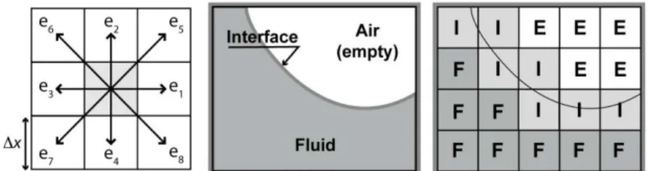
The LBM consists in applying the Boltzmann equation to the fluid, which is modelled as a collection of fluid particles moving on a fixed rectangular grid. To model free surface flows in two dimensions, the so-called D2Q9 model (2 dimensions, 9 velocities) is used along with the “mass tracking” approach (Figure1)[23].
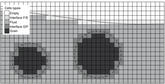
Figure 1. Left: D2Q9 scheme and Right: discretization of the flow domain according to cells types.
The flow domain is discretized in square cells of linear size x, to which are associated a position vector x, a density
xt, and a velocityu
xt, . At each time step, the density and velocity are transported from one cell to its 8 neighbouring cells (i=1,…,8) or remain within the cell (i=0). To each of the nine possible directions i, are associated a local density distribution function fi, and a velocity ui such that
i i i i i t f t t f t , , , , x u x u x x (1)
with ui=u ei where u=x/t.At each time step, two main operations are performed on flow particles: collision and streaming. These are briefly recalled below (see e.g. [27] or [22] for more details).
Streaming:
The particles with local density fi
x,t located at position x at time t, move with velocityui to the point x+uit during a time step t:
tt t
f
tfi xui, i x,
(2)
Collision:
It is assumed that the particles with density fi
x,t entering simultaneously the same cell will collide with each other, yielding a new distribution function fi
,tout x defined by the BGK model [27]:
, , 1 , , eq out u x x x i i i i t f t f t f f (3)
where is a dimensionless relaxation time and the eq
i
f are the equilibrium distribution functions given by
u e u
e u
uu 2 2 4 2 eq 2 3 2 9 3 1 , c c c w fi i i i(4)
where the wi are density weights (w0=4/9; wi=1/9 for i=1…4 and wi=1/36 for i=5…8). Boltzmann equation:
Equations (2) and (3) are combined to give the Boltzmann equation that includes a supplementary term proportional to the external force F:
vF c t w f t f t f t t t f i s i i i i i i 2 in eq in , , 1 , , x u x u x(5)
where cs is the so-called sound speed of the Boltzmann network, given by c2s u2/3. Treatment of the free surface:
The free surface is taken into account by introducing 3 types of cells: fluid, empty and interface (Figure 1). Interface cells are partially filled cells that separate the air (empty
cells) from fluid. The mass tracking approach [23] consists in tracking the movement of the
fluid interface by the calculation of the mass exchange mi between interface cells and their neighbours. This flux can be directly computed from the fi movement at the streaming step. For each given direction i, three configurations can occur according the type of the neighbour cell (located at x+uit):
- Type E (empty cell). The mass exchange is null:
,
0mi xt t
(6)
- Type F (totally filled cell). The mass exchange is simply:
t t
f
t t
f
tmi x, ~i xui, i x,
(7)
where ~i represents the opposite of direction i. The first (resp. second) density function is the amount of fluid that is entering (resp. leaving) the interface cell.
- Type I (interface cell). The mass exchange between two interface cells must account for the quantity of fluid contained in the cells (fluid fraction ε = m/):
2 , , , , , ~ t t t t f t t f t t mi i i i i x u x x u x x (8)
A more precise computation of the mass exchange can be done for this third case according to the type of the two cells neighbours. It is not presented here for the sake of conciseness but can be found [24].
The mass exchange is computed for each neighbouring cell and the mass is thus updated to:
8 1 , , , i i t t m t t t mx x x(9)
Note that, at the end of this step, some interface cells can be emptied or filled. The cell type is thus changed accordingly and the lacking or exceeding mass is reallocated to neighbouring cells.
Example:
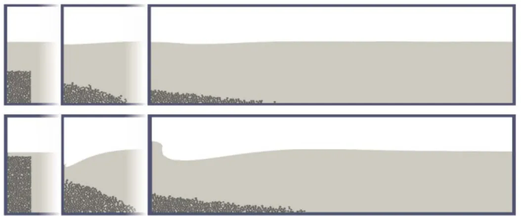
Figure 2 shows an example of free surface simulation. Results obtained for the classical dam-break problem are in very good agreement with those obtained from experimental test cases such as proposed in [7]. For the sake of comparison with [7] the classical non dimensional variable Tt g/ h0 is used, where h0 is the initial water depth in the left side of the dam.
Figure 2. Dam-break on dry bed. Screen capture taken at T=0, T=0.88, and T=1.57 (these simulations are in good agreement with experimental results given in figure 3 of [7]).
2.2. Grain modelling: sample construction and DEM computation
The Discrete Element Method is used to build a densely-packed sample of polydisperse spherical grains. A set of grain diameters according to the cumulative beta distribution is obtained with the statistical model proposed by [25]. The beta distribution has the advantage to be bounded on both sides and capable of representing double-curved distributions similar to the soil grain-size distributions encountered in practice.
Once the diameters are generated, the grains are first placed on a regular grid in a rectangular column as a dilute sample and then compacted between two plates using the procedure proposed in [18].
The force F between two grains is defined by F=(N,T) where the normal part N is due to the contacts between particles and the tangential part T stems from friction. A linear-elastic approximation is used to represent the force law between a pair (i,j) of contacting particles:
otherwise 0 0 for 2 ij ij n n ij N n mk k N (10)
where is the gap or the overlap between the two contacting particles i and j and its
derivative with respect to time, kn is the normal stiffness, m=mimj/(mi+mj) is the reduced mass and
0,1 is a damping parameter which controls energy dissipation due to inelastic collision. The friction is computed with the classical Coulomb law expressed as a nonlinear relation between the friction force T and the sliding velocity.
v N n T t f , minwhere is the tangential viscosity parameter, f is the friction coefficient and vt the tangential velocity at contact.
2.3. Coupled LBM/DEM model for fluid/solid interactions
Solid particles (grains) previously generated are introduced in the fluid domain of LBM using the same discretization scheme. Since in two dimensions the poral space does not percolate through the sample, for the fluid computation, we reduce the diameters of the grains in order to have a minimum of two nodes of fluid at contact between grains. A new type of cell is thus used: G for grain cell (see figure 3). As for free surface, the interaction between fluid and solid particles appears only at the interface.
Figure 3. Grains and fluid discretization (cells types).
Grains are considered as moving boundaries on which the non-slip condition is imposed to the fluid using the standard bounce back rule. The hydrodynamic forces acting on grains are computed using the momentum exchange method proposed by [9]. The fluid particles that are bounced back on grain boundaries transmit forces to the grain proportionally to their momentum change [1][11]. The implementation of this method is straightforward since particles momenta are known at each time step. The total hydrodynamic forces exerted on a solid particle are obtained by summing up the forces on all boundary nodes of that particle. Finally, these forces are used to compute the motion of grains.
Example:
Figure 4 shows the velocity of a grain in freefall in comparison with theoretical results given by the second Newton’s law and a friction law of the form f=-ku2 valid for an inertial regime i.e. for a Reynolds number greater than one, which is the case here.
0 0.02 0.04 0.06 0.08 0.1 0 0.1 0.2 0.3 0.4 0.5 LBM/DEM Theory t (s) u (m/s)
Figure 4. Validation of the grain fall velocity in water. The theoretical curve is obtained with a friction law of the form f=-ku2s.
III. NUMERICAL EXPERIMENT AND RESULTS
For the sake of conciseness and clarity, only qualitative results are presented here. A more precise physical interpretation as well as parameter study will be presented in detail in further work.
Figure 5. Collapse of a grain column. Up: ratio column height/water depth = 0.508 (spl05). Down: ratio=0.915 (spl09). Screen captures taken at T=0, T=0.04 and T=0.08.
The methodology is used to assess the effect of the collapse of a grain column in water, on the generation of wave surface. The domain is chosen long enough to avoid the influence of the right-hand boundary condition and wave reflection. The initial water depth h0 is the same in each test case. Five grains samples (spl09; spl08; spl07; spl06; spl05) have been generated with the following ratio of column height over initial water depth: hc/h0=(0.915; 0.813; 0.711; 0.610; 0.508). The column width remains identical for the five samples, corresponding to approximately ten grains. The total number of grains for the different samples is respectively N=(407; 360; 316; 275; 229). Figures 6 gives simulation results of a grain column collapsing in water at different non-dimensional time Tt g/ h0 . This test
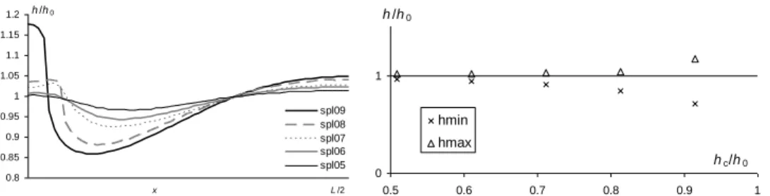
has been performed with five different column heights and the same water depth. The ratio of the water depth over the initial water depth at T=0.08 has been reported in Figure 5 for each test case as well as the maximum and minimum water depth at T=0.08 as a function of the initial granular column height. As could be expected, the amplitude of the generated wave increases with the granular column height. It can also be seen in Figure 6 (left) that the extreme values are not located at the same abscissa. Further studies will allow for a more precise parameter analysis to be conducted.
0.8 0.85 0.9 0.95 1 1.05 1.1 1.15 1.2 spl09 spl08 spl07 spl06 spl05 x L /2 h /h0 0 1 0.5 0.6 0.7 0.8 0.9 1 hmin hmax hc/h0 h /h0
Figure 6. Left: ratio of water depth h at T=0.08 over the initial water depth h0 for the different samples. Right:
minimum and maximum water depth as a function of the initial granular column height (all values being normalized by h0)
IV. CONCLUSION
The presented work gives the basis for the simulation of fluid/grain interactions in presence of free surface. The methodology has first been validated for simple cases. The dam-break test case (without grain) gives similar results to those experimentally obtained in the literature. The falling velocity of a unique grain in free fall has been successfully compared to theoretical laws.
As a first parametric analysis, we assessed the influence of the initial column height on the amplitude of the wave generated at the free surface. Other parameters will also be studied such as the aspect ratio of the grain column, grain distribution characteristics, etc. An interesting problem is also to investigate the triggering of the collapse using a cohesive model for the contact of granular materials such as proposed in [4].
The comparison of the proposed methodology with experimental results obtained in [7] or [28] for dam-break upon sediments is also one of the forthcoming goals of this work. REFERENCES
[1] Bouzidi M., Firdaouss M., Lallemand P., “Momentum transfer of a Boltzmann-lattice fluid with boundaries”. Physics of Fluids, 13, 3452-3459 (2001).
[2] Cassar C., Nicolas M., Pouliquen O., “Submarine granular flows down inclined planes”. Physics
of fluids 17, 103301 (2005).
[3] Courrech du Pont S., Gondret P., Perrin B. et al., “Granular Avalanches in Fluids”. Physical
Review Letters, 90 (2003).
[4] Delenne J.-Y., El Youssoufi M.S.; Cherblanc F. et al., “Mechanical behavior and Failure of cohesive granular materials”, Int. J. Numer. Anal. Meth. Geomech., 28, 1577-1594 (2004). [5] Delenne J.-Y., Mansouri M., Radjaї R. et al., “Onset of Immersed Granular Avalanches by
DEM-LBM Approach”, Advances in Bifurcation and Degradation in Geomechanics and
[6] Delis A.I., Kazolea M. “Finite volume simulation of waves formed by sliding masses”, Int. J.
Numer. Meth. Biomed. Engng. 27, 732–757 (2011)
[7] Duarte R., Ribeiro J. Boillat J.-L. et al., “Experimental study on dam-break waves for silted-up reservoirs” Journal of Hydraulic Engineering ASCE, 137, 1385-1393 (2011)
[8] Grilli S.T., Watts P., “Modelling of waves generated by moving submerged body. Applications to underwater landlide.” Engineering Analysis with Boundary Elements, 23, 645 (1999). [9] Ladd A.J.C., “Numerical simulation of particular suspensions via a discretized Boltzmann
equation, Part 2, Numerical results”, J. Fluid Mech. 271, 311-339 (1994).
[10] Lajeunesse E, Monnier J.B., Homsy G.M., “Granular slumping on a horizontal surface”, Physics
of fluids 17, 103302. (2005).
[11] Lallemand P., Luo L.-S., “Lattice Boltzmann method for moving boundaries”, Journal of
Computional Physics, 84, 406-421 (2003).
[12] Legros, F. “The mobility of long-runout landslides”, Engineering Geology 63 301-331 (2002). [13] McAdoo B.G., Watts P, “Tsunami hazard from submarine landslides on the Oregon continental
slope”, Marine Geology, 203, 235-245, (2004).
[14] McNamara S., Flekkoy E. G., Maloy K. J., “Grains and gas flow: Molecular dynamics with hydrodynamic interactions”, Physical Review E, 62, 4 (1999).
[15] Mangeney-Castelnau A., Bouchut F., Vilotte J.P. et al., “On the use of Saint Venant equations to simulate the spreading of a granular mass”, J. Geophys. Res., 110 (2005).
[16] Mansouri M., Delenne J.-Y., El Youssoufi M. S. et al., “A 3D DEM-LBM approach for the assessment of the quick condition for sands”, C.R. Mecanique 337, 675-681 (2010).
[17] Mason D., Habitz C., Wynn R. et al., “Submarine landslides: processes, triggers and hazard protection”, Philosophical Transactions of the Royal Society, 364, 2009–39, (2006).
[18] Schafer J., Dippel S., Wolf D.E., “Force schemes in simulations of granular materials”, Journal
de Physique 6, 5–20 (1996).
[19] Spinewine B., Guinot V., Soares-Frazao S. et al. “Solution properties and approximate Riemann solvers for two layer shallow flow models”. Computers & Fluids, 44, 202-220, (2011).
[20] Staron L., Hinch E.J., “The spreding of a granular mass: role of grain properties and intial conditions”, Granular Matter 9, 205-217, (2007).
[21] Sue L.P.Nokes R.I., Davidson M.J., “Tsunami generation by submarine landslides: comparison of physical and numerical models”Environ Fluid Mech 11, 133–165 (2011).
[22] Sukop M.C., Thorne D.T. Lattice Boltzmann Modeling. Springer (2006).
[23] Thürey N., Rüde U., “Stable free surface flows with the lattice Boltzmann method on adaptively coarsened grids” Computing and Visualization in Science, 12 (5): 247-263, (2009).
[24] Thürey N., Körner C., Rüde U, “Interactive free surface fluids with the Lattice Boltzmann Method”. Technical Report 05-4. University of Erlangen-Nuremberg, Germany, (2005). [25] Topin V., Dubois F., Monerie Y. et al., Micro-rheology of dense particulate flow: application to
immersed avalanches. Journal of Non-Newtonian Fluid Mechanics 166, 63-72 (2011).
[26] Voivret C., Radjai F., Delenne J.-Y. et al., “Space-filling properties of polydisperse granular media”. Phys. Rev. E Stat. Nonlin. Soft Matter Phys. 76, 021301 (2007).
[27] Wachs A., “A DEM-DLM/FD method for direct numerical simulation of particulate flows: Sedimentation of polygonal isometric particles in a Newtonian fluid with collisions”, Computers
and Fluids, 38, 1608-1628 (2009).
[28] Zech Y., Soares-Frazao S., Spinewine B. et al., “Dam-break induced sediment movement: Experimental approaches and numerical modeling” Journal of Hydraulic Research, 46, 176-190 (2008).
[29] Zhou J.G. Lattice Boltzmann Methods for Shallow Water Flows. Springer, softcover reprint of hardcover 1st ed. 2004 edition, 11 (2010).
![Figure 2 shows an example of free surface simulation. Results obtained for the classical dam-break problem are in very good agreement with those obtained from experimental test cases such as proposed in [7]](https://thumb-eu.123doks.com/thumbv2/123doknet/13524748.417309/5.893.170.721.551.635/simulation-results-obtained-classical-agreement-obtained-experimental-proposed.webp)