HAL Id: hal-00533562
https://hal.archives-ouvertes.fr/hal-00533562
Submitted on 9 Nov 2010
HAL is a multi-disciplinary open access
archive for the deposit and dissemination of
sci-entific research documents, whether they are
pub-lished or not. The documents may come from
teaching and research institutions in France or
abroad, or from public or private research centers.
L’archive ouverte pluridisciplinaire HAL, est
destinée au dépôt et à la diffusion de documents
scientifiques de niveau recherche, publiés ou non,
émanant des établissements d’enseignement et de
recherche français ou étrangers, des laboratoires
publics ou privés.
Progressive Lossless Mesh Compression Via Incremental
Parametric Refinement
Sébastien Valette, Raphaëlle Chaine, Rémy Prost
To cite this version:
Sébastien Valette, Raphaëlle Chaine, Rémy Prost. Progressive Lossless Mesh Compression Via
In-cremental Parametric Refinement. Computer Graphics Forum, Wiley, 2009, 8 (5), pp.1301-1310.
�10.1111/j.1467-8659.2009.01507.x�. �hal-00533562�
Eurographics Symposium on Geometry Processing 2009 Marc Alexa and Michael Kazhdan
(Guest Editors)
Volume 28(2009), Number 5
Progressive Lossless Mesh Compression Via Incremental
Parametric Refinement
Sébastien Valette1, Raphaëlle Chaine2and Rémy Prost1
Université de Lyon, CNRS
1CREATIS-LRMN; UMR5220; Inserm U630; INSA-Lyon; Université Lyon 1, France 2Université Lyon 1, LIRIS, UMR5205, F-69622, France
Abstract
In this paper, we propose a novel progressive lossless mesh compression algorithm based on Incremental Para-metric Refinement, where the connectivity is uncontrolled in a first step, yielding visually pleasing meshes at each resolution level while saving connectivity information compared to previous approaches. The algorithm starts with a coarse version of the original mesh, which is further refined by means of a novel refinement scheme. The mesh refinement is driven by a geometric criterion, in spirit with surface reconstruction algorithms, aiming at generat-ing uniform meshes. The vertices coordinates are also quantized and transmitted in a progressive way, followgenerat-ing a geometric criterion, efficiently allocating the bit budget. With this assumption, the generated intermediate meshes tend to exhibit a uniform sampling. The potential discrepancy between the resulting connectivity and the orig-inal one is corrected at the end of the algorithm. We provide a proof-of-concept implementation, yielding very competitive results compared to previous works in terms of rate/distortion trade-off.
1. Introduction
Technological advances have pushed 3D graphics to higher levels of realism, and improvements are still emerging at a steady pace. The range of applications using 3D meshes for shape representation stretches from the visualization of to-pographic data on supercomputers to video games on cellu-lar phones. With the eventual bandwidth limitations on such applications, 3D mesh compression has gained a lot of in-terest in the last 20 years. In this paper, we propose a novel 3D progressive lossless mesh compression paradigm, from which we derive an initial implementation (not suited for all the mesh classes) with the following characteristics: • atomic granularity : starting from the coarse resolution
mesh, new vertices are inserted in the triangulation one at a time, until the original mesh is completely recon-structed.
• the intermediate resolution meshes have their vertices well distributed over the surface.
• the mesh triangles exhibit good aspect ratio, as the mesh conforms to a local Delaunay criterion.
2. Background on mesh compression
The triangular mesh representation can be split in two dif-ferent informations : geometry i.e. a 3D set of point coordi-nates, and connectivity i.e. a list of triangles connecting the points. Following Tutte’s work [Tut62], the amount of in-formation needed to encode the connectivity of a triangular mesh is bounded by the Tutte entropy ETutte = 3.245 bpv.
The first works on mesh compression were done by Deer-ing [Dee95], followed by the algorithm of Touma and Gots-man [TG98], where a canonical walk on the triangle mesh allows to encode the mesh connectivity by storing the ver-tices valences and non-frequent incidents codes. It has been shown to be very close to optimality [Got03]. Rossignac [Ros99] proposed an approach with a worst-case bound on its coding cost : Edgebreaker, which codes the mesh connec-tivity on 2 bits per triangle. Finally, Poulalhon and Schaef-fer [PS06] have provided an approach based on Schneider tree decomposition, with a coding cost equal to the Tutte entropy. Single-resolution approaches usually combine one of the previously cited approaches or their derivatives for the mesh connectivity, and use the connectivity to improve geometry coding by means of prediction, the most widely
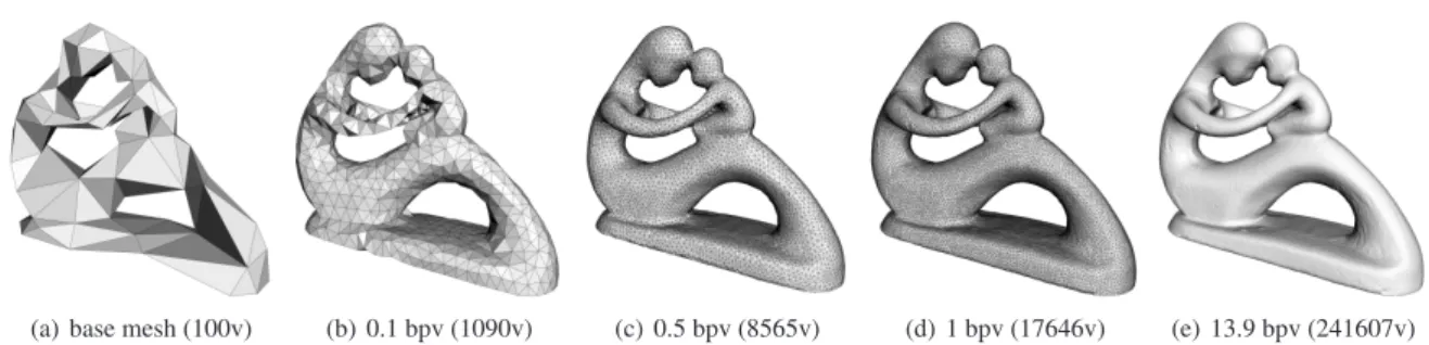
(a) base mesh (100v) (b) 0.1 bpv (1090v) (c) 0.5 bpv (8565v) (d) 1 bpv (17646v) (e) 13.9 bpv (241607v)
Figure 1: IPR-based Progressive transmission of the Fertility model (241k vertices). Note the uniform sampling and visual
quality of the intermediate meshes (b), (c) and (d).
known being the parallelogram prediction. The vertices co-ordinates are usually quantized to 10 or 12 bits per coordi-nate, can be losslessly encoded, such as proposed by Isen-burg et al. [ILS05], and can be used to predict the connectiv-ity, thus improving compression rates [LCL∗06].
Progressive compression approaches start with the cod-ing of a coarse approximation of the original mesh and add information allowing to progressively reconstruct the original mesh by means of refinements. First approaches have focused on connectivity refinement : Cohen-or et al. [COLR99] start from the original mesh and iteratively re-move its vertices in carefully selected batches until the low-est resolution is obtained. The reconstruction is guaranteed by a 4-colour coding scheme. Taubin et al. [TGHL98] pro-posed a tree-based refinement scheme called progressive for-est split. The vertex-split based progressive meshes scheme proposed by Hoppe [Hop96] has been used in [PR00] and [KBG02] to encode vertex splits in batches. When one only wants to store the shape of the object represented by the mesh, the connectivity can be changed to a much simpler one, a structured connectivity, whose coding cost is neg-ligible compared to an irregular connectivity and is a per-fect fit for geometry compression via transform coding. Effi-cient progressive geometry compression using uniform sub-division was first proposed by Khodakovsky et al. [KSS00] and Guskov et al. [GVSS00]. Payan and Antonini [PA05] proposed an optimized bit-allocation algorithm within this framework. Gu et al. [GGH02] proposed to resample the original mesh to a regular connectivity mesh, a geometry image. This work was further improved by Peyre and Mal-lat [PM05] by taking into account local anisotropy in the shape to be encoded. An other approach using transform coding is the spectral compression introduced by Karni and Gotsman [KG00]. When the original mesh connectivity mat-ters, using transform coding algorithms for geometry com-pression is not straightforward, as these methods are based on regular mesh subdivision. To solve the problem faced when compressing irregular connectivity, Alliez and Des-brun [AD01] try to reverse√3 subdivision on the input mesh [Kob00], while the Wavemesh coder proposed by Valette and Prost [VP04] tries to reverse face quadrisection. For both
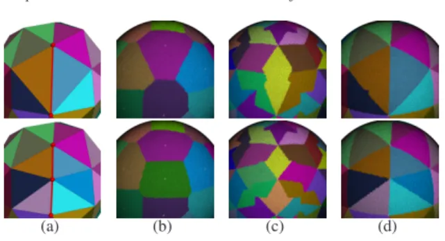
approaches, when the regular subdivision is not applicable, incident codes need to be transmitted and generate coding overhead. As a consequence, compression efficiency of these approaches is highly dependent on the regularity of the in-put mesh. Note that these approaches try to keep the mesh connectivity as regular as possible during the simplification step, but finding the optimal simplification rules is still an open problem. Finally, the most recent progressive coders are not only driven by connectivity refinement, but also by geometric measures on the reconstructed mesh. Gandoin and Devillers [GD02] propose to encode the vertices coordinates with a Kd-tree coder, with the side-effect of efficient con-nectivity compression by means of generalized vertex splits. This approach allows complex connectivity operations and is therefore able to handle meshes with complex topology such as polygon soups. Peng and Kuo [PK05] further im-proved this approach by replacing the Kd-tree with an octree data structure. The octree cells are refined in a prioritized or-der, where the cells subdivisions offering the best distortion improvement are performed first. These approaches provide good results for lossless compression, but they are based on structured volume hierarchies which induce anisotropy and blocking artifacts, thus reducing rate-distortion performance at low bitrates (figure2.(c)).
3. Outline of our approach
We propose to redefine the problem of progressive mesh transmission into a mesh generation problem. Figure 2
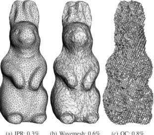
shows a comparison between our Incremental Parametric Refinement (IPR) approach, Wavemesh [VP04] and the Oc-tree Compression method [PK05]. At 1bpv, our approach generates a visually pleasing mesh, while the reconstruction with Wavemesh at 1.42 bpv exhibits stretched triangles and a higher approximation error (0.6% of the model Bounding Box Diagonal Length). At 1bpv, the Octree Compression approach outputs a mesh with the worse visually pleasing properties and higher approximation error (0.8%). The prob-lem of surface meshing has been widely studied in the last years [AUGA07]. We use a refinement scheme driven by a Delaunay mesh generation approach, which produces
uni-S. Valette, R. Chaine & R. Prost / Progressive Lossless Mesh Compression Via Incremental Parametric Refinement 3
(a) IPR: 0.3% (b) Wavemesh: 0.6% (c) OC: 0.8%
Figure 2: the rabbit model compressed down to 1 bit per
original vertex with our approach (a) and the Octree Com-pression (c), and at 1.42 bpv with Wavemesh (b). The percentages represent the approximation error in terms of Hausdorff distance, with regard to the mesh bounding box diagonal length.
form triangulations during progressive transmission at low coding cost, as most of the connectivity is implicitly defined by the reconstruction algorithm. Note that an alternate ap-proach using reconstruction algorithms has been proposed by Chaine et al. [CGR07] to predict the mesh topology, but it is limited to connectivity encoding, assuming that the vertices coordinates are already available. Our approach si-multaneously encodes the vertices coordinates and the mesh connectivity and avoids the use of any volumic data struc-ture. Subsequently, we note the input mesh as M and n its number of vertices. We assume in this paper that the final reconstructed mesh will have the same connectivity as the original mesh, and each vertex coordinate will be quantized to a given number Nqof bits. The coding will consist in
start-ing from a base mesh Mbwhere b is its number of vertices
(b << n). The set of vertices of Mbis a subset of the
ver-tices of M, and their coordinates are quantized on Nbbits
(Nb< Nq). Afterwards, Mbis iteratively refined by
insert-ing the missinsert-ing vertices in order to construct a sequence of meshes Mb,Mb+1,Mb+2, ...,Mn−2,Mn−1,Mn
Finally, when all the vertices of M have been transmitted, we need to ensure that the connectivity of the reconstructed mesh is the same as the original. This is done by iteratively flipping some edges of Mnuntil it matches M.
Our scheme takes into account the following assumptions: • A fine to coarse approach for connectivity encoding de-creases coding efficiency, as only the final mesh connec-tivity has to conform to the input mesh connecconnec-tivity.
In-stead, a coarse to fine approach can improve compression at low bitrates, as when the current mesh Mi has
rela-tively few vertices (i ≪ n), every operation should create a new vertex (and never require incident codes), similarly to uniform subdivision schemes.
• In spirit with the octree-based coder [PK05], the effi-ciency of progressive transmission can be improved with a careful prioritization of refinement sites.
• For each resolution level Miwhere b ≤ i ≤ n, we need
to provide a good trade-off between the level of quantiza-tion of the vertices coordinates and the number of vertices in the mesh, as pointed by King and Rossignac [KR99]. Hence, if the final vertices are coded on Nq bits, we can
encode the vertices of coarser resolution levels with a lower number of bits. The remaining bits with low signif-icance are transmitted latter in the refinement sequence, similarly to the SPIHT coder [SP96].
For this aim, we propose a decoder-centric template In-cremental Parametric Refinement (IPR) algorithm which is instantiated with output writing operations for the compres-sion step, and input operations for the decomprescompres-sion. This algorithm performs a good balance between vertices quan-tization and connectivity evolution at each resolution level Miwith two independent measures:
• An estimate of the adequate number of bits needed to rep-resent the coordinates of a given vertex. This number is computed by IPR and grows during refinement until full precision is reached.
• A prediction of the refinement sites. At each resolution level i, the algorithm can predict which region is a good candidate for refinement i.e. the location where increasing the sampling density is likely to lower the approximation error.
4. Description of the IPR algorithm
In this section, we develop the idea behind our paper : For each resolution level, IPR carefully chooses the location of the next refinement, and transmits the coordinates of the ver-tex used for the refinement, using differential coding. We exploit the statistical fact that a way to reduce the approx-imation error for a given sampling is to refine the regions having the lowest sampling density. Also, at any time, the algorithm can request some data to refine the coordinates of a given vertex. Again, compression and decompression are performed using the same algorithm, except that com-pression writes data and decomcom-pression reads the data. As a consequence, the data requests do not need explicit com-munication between the decoder and the encoder, only the requested data needs to be transmitted in the bitstream.
4.1. A new surface-aware refinement scheme
We propose an incremental refinement scheme which aims at constructing uniform triangulations by means of simple
Algorithm 1: IPR base algorithm. begin
Set Mi= Mb;
Fill the priority queue Queue1 with the edges of Miand their respective length as priority value ;
repeat
Pop a candidate edge e from Queue1;
if e needs to be split (read/write one bit) then
Add a new vertex at the edge midpoint (read/write delta coordinates) and two new triangles;
Restore Delaunay property of Mi;
Update the priority of flipped edges in
Queue1;
Mibecomes Mi+1;
end
if Queue1 is empty then
Fill Queue1 with the edges of Miand their
respective length as priority value ;
end until i= n ;
end
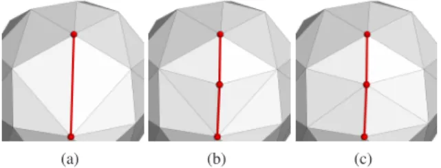
atomic operations. Each operation consists in an edge split followed by an automatic local Delaunay enforcement step, as shown by figure3. At a given resolution level i, we pick the longest edge e of Mi, in order to increase the sampling
density of the surface (figure3.(b)) while preserving unifor-mity. This operation requires the insertion of a new vertex vi
into the triangulation. The position of e does not need to be transmitted, as it is computed by both the decoder and en-coder. At the encoder end, viis chosen among the vertices of
M with the goal of getting the best approximation improve-ment.
Then, after each vertex insertion, the quality of the trian-gulation is increased, using a local Delaunay criterion, such as proposed by Dyer et al. [DZM07]. This consists in per-forming local checks on all modified edges and their neigh-boring edges: for each edge e to check, we measure the De-launay criterion De= α + β − π, where α and β are the
values of the opposite angles of e. A positive value for De
means that e is not a local Delaunay edge and therefore has to be flipped. Note that flipping an edge can also change its neighboring edges Delaunay criterion value. Consequently, we also have to check that the Delaunay criterion is also re-spected for this neighborhood and repeat these operations until all the edges satisfy the criterion. The whole scheme is easy to implement using a priority queue, and its conver-gence is guaranteed [DZM07]. An efficient way of keeping track of the longest edge in Mi is to use an other priority
queue whose average construction and update complexity is in n log n.
Moreover, we prevent the edge flips that would cause the
(a) (b) (c)
Figure 3: the proposed refinement scheme : (a) an edge e
(in bold red) is selected for refinement. (b) It is split in two, resulting in the creation of a new vertex and two new trian-gles. (c) The resulting triangulation is modified in order to satisfy a local Delaunay Property, by means of edge flips. In this example, two edges have been flipped.
underlying geometry to change significantly. For each edge
eto be flipped, we measure the volume veand area aeof
the tetrahedron formed by the two vertices of e and the two vertices opposite to e, and compute the flip criterion Fe=
3
√ve √a
e. Whenever Feis above a given threshold Ft, we forbid
the flip. In our experiments, we set Ft= 0.3.
Finally, the cost of one refinement operation is reduced to the localization of the edge to split and the additional geo-metric information needed to create the new vertex. Connec-tivity evolves automatically, without any overhead data.
Our refinement algorithm takes into account the geomet-ric properties of the evolving reconstructed mesh, but the operations and criteria used here are only performed in the mesh parametric domain, in contrast with volumetric subdi-vision approaches such as [GD02,PK05], hence the name
Incremental Parametric Refinement. This scheme allows for
faithful progressive approximation of the original model, even at low bitrates.
4.2. Predicted splits for connectivity encoding
The proposed scheme can encode the mesh connectivity in a very efficient way. The challenge here is to decide for a resolution level i whether the longest edge e needs to be split or not at the decoder end. This implies a mapping between the original mesh vertices and the reconstructed mesh edges. Each edge ejof Miwill be associated with a set Vjof
ver-tices in M not present in Mibut which are candidates for
insertion by splitting ej in Mi. As the resolution level
in-creases, the set Vjcontains less and less vertices, and will
eventually become empty. As a result, when the set is empty, we need to prevent the edge split. Note that at a given res-olution level, it can happen that the set of candidates Vjfor
ejis empty, but it can later be given new candidate vertices
after edge flips occur in its neighborhood.
Therefore, for each selected edge e, we need to trans-mit one bit (1 for yes, 0 for no), so that the decoder knows
S. Valette, R. Chaine & R. Prost / Progressive Lossless Mesh Compression Via Incremental Parametric Refinement 5
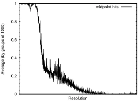
Figure 4: Values of midpoint codes when compressing the
Fertility model : the moving average value is very close to 1 at the beginning of the transmission and gradually vanishes as the resolution increases.
whether e must be split or not. Subsequently, we will call these informations midpoint codes. If the picked edge is not split, the same test is performed with the next longest edge in the queue, until a to-be-split edge is encountered. After each split, the resolution level is incremented. At low reso-lution levels, the midpoint codes will most frequently have the value 1, and will most often be 0 at high resolution lev-els. This is illustrated by figure 4which shows the mid-point codes average values, by order of appearance, com-puted for groups of 1000 successive values when compress-ing the Fertility model. We can then improve the compres-sion efficiency using adaptive arithmetic coding with a rel-atively short statistics update interval (the so-called rescale interval). In our experiments, we have set the rescale inter-val to 15. As an example, when compressing the fertility model, 987141 midpoint codes are needed. The entropy of this bitstream is 0.89 bits per midpoint code, but using adap-tive coding reduces the coding cost to 0.36 bits per midpoint code. This translates to a relative coding cost of 1.45 bits per vertex.
4.3. Quantization/connectivity trade off
The quantization of vertices coordinates plays a key role for efficient mesh compression. Indeed, it is well known that the size of the geometric information is much bigger than the size of connectivity information. As explained in sec-tion2, connectivity-driven compression approaches such as Wavemesh usually encode and transmit vertices coordinates in a constant-quantization way, whereas recent compression schemes such as the Octree Compression approach refine the vertices coordinates as the resolution increases. But Octree and Kd-tree approaches still do not provide the good bal-ance between the number of vertices in the mesh and the level of quantization of vertices coordinates. This is clearly illustrated by figure2.(c) : at 1bpv, the Octree Compression delivers a mesh made of 12959 vertices, but the vertices co-ordinates quantization is too coarse to provide a good
ap-Figure 5: comparison of rate-distortion performance when
compressing the balljoint model, for various values of qt
proximation of the rabbit model. Instead, in figure2.(a) our approach reconstructs a more accurate mesh with only 4833 vertices, but with a higher number of bits transmitted for the vertices coordinates. At this resolution level, 78% of the ver-tices coordinates are coded with 11 bits precision, and the re-maining are coded with 12 bits. More generally, each vertex
viis given a specific quantization level Qiwith 0 < Qi< Qm
where Qmis the maximal quantization level (usually 12 bits).
The quantized coordinates eciof a given vertex viare
com-puted as: e ci= j 2Qi−Qmc i k (1) We propose to first transmit the coordinates of the base mesh vertices with a low number of bits (Nb= 4 in our
experi-ments), and let the IPR algorithm choose whether the quan-tization level Qiis sufficient or not for a given vertex vi. This
is done by measuring the squared distance Di(in its
quan-tized version) between viand its closest neighbor vertex vj:
Di=
eci− ecj
2 (2)
Where ciare the coordinates of the vertex vi. Whenever
Diis lower than a threshold qt, the quantization precision is
increased by one bit (if full precision has not already been reached). This results in transmitting one bit of refinement for each coordinate of vi. When a new vertex viis inserted in
Miby splitting the edge e, its quantization level is set to the
average between the quantization levels of the vertices of e, and only the difference between the edge midpoint and the actual coordinates of viis transmitted, thus reducing the
en-tropy of the data to transmit. The resulting delta-coordinates are entropy coded by means of arithmetic coding. Eventu-ally, when a new vertex is inserted in the mesh, the quan-tization criterion will not be satisfied, and the coordinates of surrounding vertices will be refined. When all the mesh vertices are inserted i.e. when Mnis reconstructed, we
re-fine the vertices coordinates which have not been transmitted with the desired final precision.
as-sume that the coordinates to encode are between 0 and 127, with qt= 600: two vertices v1 and v2with coordinates 80
(1010000 in binary) and 30 (0011110 in binary) are currently coded with a precision of 4 bits, which results in quantized values of 10 (1010 in binary) and 3 (0011 in binary), the 4 most significant bits for both coordinates. The squared dif-ference between this numbers is 49, which is less than qt.
Increasing the precision to 6 bits will make the coordinates become 40 (101000 in binary) and 15 (001111 in binary) which satisfy the quantization criterion, as (40−15)2= 625. Figure5shows the rate-distortion compression curves ob-tained with our approach when compressing the balljoint model, for various values of qt. This parameter improves
the efficiency of our approach by about 20% at intermedi-ate level, but also increases the amount of data needed for the final lossless compression. In our experiments, we have set qt to the conservative value of 600, which still offers a
gradually increasing precision with no significant overhead for lossless compression.
Finally, on figure1.(b), the reconstruction of the fertil-ity model at a bitrate of 0.1bpv has 1090 vertices. 54% of the coordinates are encoded with 10 bits, 43% with 11 bits, and the remaining 2% with more precision. This results in an RMS error of 1.96 while constant quantization (when
Nb= Qm= 12) results in an error of 3.45 for the same
bi-trate. For the rabbit model at 1 bpv, adaptive quantization results in an error of 4.4 while constant quantization leads to an error of 5. Moreover, figure9(right) shows that for bi-trates below 2bpv, adaptive quantization improves compres-sion compared to constant quantization.
4.4. Getting the original connectivity back
When the highest-resolution mesh Mnis reconstructed, we
still need to modify its connectivity Tnso that it matches the
triangulation of M, noted T . The problem of finding a finite sequence of edge flips to change a genus-0 triangulation into an other genus-0 triangulation has been solved for the unla-beled case by Wagner [Wag36] and by Gao et al. [GUW01] for the labeled case (our case) but finding the flip sequence with minimal size is still an open problem. Currently avail-able solutions use a canonical triangulation as a mandatory intermediate connectivity on the path between Tnand T and
therefore perform a high number of flips. As we want the smallest number of flips as possible for compression effi-ciency reasons, instead of using an of-the-shelf algorithm, we propose to use an heuristic approach, taking into account the fact that in our case, Tnand T should be very similar.
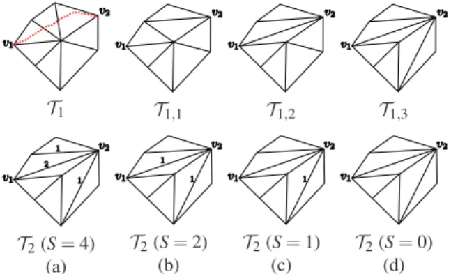
We define an asymmetric measure of similarity S between two triangulations T1and T2as:
S(T1→ T2) =
∑
ei∈E2dT1(ei,1, ei,2) (3)
where E2is the set of edges of T2. ei,1and ei,2are the
ver-tices of the edge ei. dT1(ei,1, ei,2) is the flip distance between
T1 T2(S = 4) (a) T1,1 T2(S = 2) (b) T1,2 T2(S = 1) (c) T1,3 T2(S = 0) (d)
Figure 6: Measuring the flip distance between two vertices:
the triangulationsT1 (top) andT2 (bottom) have the same set of vertices, but different connectivity. We measure the flip distance for each edge ofT2. As an example, when measur-ing the flip distance dT1(v1, v2) the shortest path between v1
and v2crosses two edges (a, top). There are only three edges inT2 with a non-null flip distance, and S(T1→ T2) = 4.
Afterwards, we perform three edge flips inT1 (b)(c)(d) to changeT1intoT1,3= T2(S(T1→ T2) = 0)
ei,1and ei,2in T1i.e. the number of flips needed to change T1
into a triangulation where the edge eiexists. We compute this
number with an algorithm similar to Dijkstra’s shortest path algorithm, where the path does not follow the mesh edges, but crosses them by walking on the dual graph. The flip dis-tance is then the number of crossed edges, which all have to be flipped when one wants to create the edge ei, as shown in
figure6.(a). Note that there can exist several minimal paths between two vertices, but this is not an issue, as with our similarity measure, we only consider the lengths of the paths and not the edges they come across. Then, we perform edge flips on Tnwith the objective to decrease S(Tn→ T ). This
translates to reducing the flip distances of the edges in T by flipping the edges in Tn.
For each edge of Mn, the algorithm transmits a single
bit informing whether the edge should be flipped or not. On the encoder end, the decision is taken based on the effect of the edge flip on S(Tn→ T ). If this value decreases, the
edge eiis flipped (coded 1). If it increases, eiis not flipped
(coded 0). If the value is the same for both cases, the en-coder performs a supplementary test : it computes the value
dT(ei,1, ei,2)) − dT(e′i,1, e′i,2)) where e′i is the edge created
when flipping ei i.e. it checks whether flipping eiwill
de-crease its flip distance (measured this time by walking on T ). If the flip distance is decreased, eiis flipped. Note that
for practical reasons, we actually do not compute all the flip distances in the mesh when computing S(Tn→ T ), but only
the flip distances of the edges incident to the four vertices involved in the edge flip.
After all the edges have been visited, the encoder checks whether the two meshes are identical, by simply verifying
S. Valette, R. Chaine & R. Prost / Progressive Lossless Mesh Compression Via Incremental Parametric Refinement 7
that S(T1→ T2) = 0. If they are identical, the encoder puts a
1 in the bitstream, otherwise a 0 and the decoder will repeat the traversal on all the edges. This procedure is repeated until the two meshes are identical. In our experiments, the number of loops on the edges is usually between 2 and 5. The num-ber of loops directly influences the bitstream entropy of our algorithm. As an example, for the Fertility model, 3 loops were required to reconstruct the original connectivity, with a relative coding cost of 2.82 bpv using arithmetic coding. In figure6, (a), (b) (c) and (d) show the complete set of flips needed to change T1into T2. the bottom part show the flip
distances computed on T2 during this transformation, and
give the value of S = S(T1→ T2).
Unfortunately, there is no guaranteed convergence for this algorithm and no proof of convexity for S. We experienced non-convergence only when the chosen order for vertices insertion was clearly wrong, resulting in a reconstructed mesh with normal flips and possibly degenerated connec-tivity. Therefore, stress has to be put on keeping the meshes Mias close as possible to the original mesh M during the
selection of transmitted vertices and on avoiding connectiv-ity drifts that can be induced with the current choice of the vertices.
4.5. Picking the right vertices order of insertion
For each resolution level i, the new vertex to insert in Miis
chosen by the encoder, so as to decrease the approximation error as much as possible. This requires a mapping between M and Mi, such as MAPS [LSS∗98] or the approach of
Schreiner et al. [SAPH04]. However, the dynamic edge flips performed during the iterative reconstruction of Miprevent
the use of such approaches in a computationally efficient way. As a first approximation, we propose a fast approach to compute the list of candidate vertices when an edge eiis
to be split. We first use a geodesic Voronoi diagram on M, with the vertices of Mi as Voronoi sites. This provides a
good mapping between the vertices of M and the vertices of Mifor each resolution level i (figure7.(b)).
Each Voronoi Region Vj is then a set of vertices of M
associated to a given vertex vjof Mi. Afterwards, we
asso-ciate each vertex vkinside a region Vjto the edge e incident
to vjgiving the maximal value for the following criterion :
C(e) = ~e
k~ek• −−→vjvk (4) i.e. we associate vkto its closest edge. The resulting
map-ping can be seen on figure7.(c). When a vertex vkhas been
associated to an edge e, it can be associated to one of the two triangles incident to e according to its position with re-gards to the plane bisecting the two triangles. The result of such mapping can be seen in figure7.(d). Finally, the list of candidate vertices for splitting an edge e is taken from the union of the vertices in M associated with the two trian-gles incident to e. When this set is empty, the edge is not
(a) (b) (c) (d)
Figure 7: Mapping between the original meshM and the
reconstructed meshMi. Top row : before edge insertion.
Bottom row : after insertion. (a) the reconstructed meshMi,
with colored triangles. (b) geodesic Voronoi Diagram onM,
with the vertices ofMias Voronoi Sites. (c) mapping
be-tween the vertices ofM and the edges of Mi. (b) mapping
between the vertices ofM and the triangles of Mi.
split. When the set is not empty, we pick the vertex which is the closest to the optimal representative vertex, computed using Quadric Error Metrics, such as proposed by Garland and Heckbert [GH97].
We conjecture that this algorithm guarantees a good ver-tices selection for convex objects, and we expect its effi-ciency to decrease when the difference between the orig-inal mesh M and the base mesh increases, i.e. when the cross-parametrization between M and Mb exhibits severe
distortions. A typical example is a protrusion or a concave region not well represented in the base mesh. More precisely, the way the encoder choses the new vertex for insertion in the reconstructed mesh Midepends mostly on the geodesic
Voronoi diagram constructed on M. However, the adjacency of the created Voronoi regions and the connectivity of Mi
sometimes differ, and this can result in a bad choice for the vertex insertion.
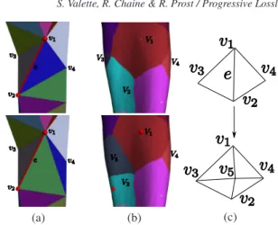
4.6. Fixing connectivity drifts
With the increase in resolution, the difference in connectiv-ity between M and Mican also increase, which can cause
normal flips on the reconstructed surface, and a mesh whose connectivity differs a lot from the original mesh connectiv-ity, thus reducing the efficiency of our approach.
To correct these potential connectivity drifts, before each edge split, we perform additional comparisons between the connectivity of Miand the connectivity of the underlying
geodesic Voronoi diagram. Let us assume that e is the edge to split, with v1 and v2 as its vertices, v3 and v4as its op-posite vertices, as shown in figure8.(c). The vertex chosen for insertion is noted v5, and it results in the creation of a new Voronoi region V5in the geodesic Voronoi diagram. As
a rule of thumb, we flip an edge between a parent vertex (v1
(a) (b) (c)
Figure 8: The reconstructed mesh connectivityMi((a), top)
does not conform the connectivity of the geodesic Voronoi di-agram onM ((b), top, one region for each vertex of Mi). We
aim at keeping this difference small. In this case, the edge e is the split location. However, the edge v2v4is flipped be-fore splitting the edge e, as the Voronoi region V4is neither adjacent to V2 nor to the Voronoi region V5 resulting from the insertion of the vertex v5. This flip reduces the difference between the connectivity ofMi((a), bottom) and the
adja-cency graph of the Voronoi diagram when v5is inserted ((b), bottom). (c) the edge split mask
vertex Voronoi region (V3or V4) is connected to none of the
Voronoi regions V5and the parent vertex region (V1or V2).
An example is shown in figure8. This operation also has to be performed by the decoder, and therefore represents over-head data to be transmitted. As a consequence, each mid-point code can have the value 0, 1 or 2, where 2 means that additional edge flips are to be performed before the edge split. In case of a ’2’ value, 4 bits need to be transmitted in order to know which edges have to be flipped. In our ex-periments, the amount of information needed for these inci-dent flips never exceeds 0.2 bpv. Note that the introduction of a more robust vertices picking algorithm will alleviate the need for such a workaround.
4.7. Base mesh construction and encoding
In order to create the base mesh Mbfrom the original mesh
M, we use an algorithm similar to Garland and Heckbert’s approach [GH97], where the edge collapse order is deter-mined by measuring the respective geometric degradation generated by each collapse. As we want the base mesh ver-tices to be a subset of the original mesh verver-tices, when col-lapsing an edge e with vertices v1and v2, we do not compute an optimal vertex position for the representative vertex, but choose the best position between v1and v2. Moreover, we
prevent edge collapses that cause normal flips on the surface or which change the topology of the mesh. For each model, the number of base mesh vertices b is arbitrarily chosen, with
Compression Dec.
Model #v I II III total total
Fandisk 6475 0.1 0.4 0.3 0.8 0.2
Horse 19851 0.7 1.4 1.7 3.8 0.5
Torus 36450 0.8 3.1 1.2 5.1 1.1
Rabbit 67039 2 7 5 14 2
Fertility 241607 8 25 27 60 9
Table 1: Timings for compression and decompression (in
seconds), where the compression is split into three parts : Base Mesh construction (I), mesh refinement (II) and Post-processing edge flips (III)
the objective of constructing a base mesh sufficiently close to the original mesh, with as few vertices as possible. When the vertices selection fails to choose the good order of ver-tices insertion, one can increase b, so as to reduce the differ-ence between Mband M. Currently, our algorithm encodes
the base mesh vertices by simply storing the vertices coor-dinates with a fixed resolution of 4 bits per vertex, which is automatically refined using the quantization criterion de-fined in section4.3. The base mesh connectivity is also sim-ply encoded by storing for each triangle the indexes of its three vertices. Note that a better compression efficiency will be reached using a coder such as the approach of Touma and Gotsman [TG98].
5. Experimental results
In this section, we compare our approach with Wavemesh [VP04], the approach of Alliez & Desbrun [AD01], the Oc-tree Compression approach [PK05] and the single-resolution coder from Touma & Gotsman [TG98]. Table1shows tim-ings for our approach on a workstation with a quad-core Intel CPU running at 2.66GHz. For the compression, we have split the timing into three parts : program initializa-tion and base mesh construcinitializa-tion (I), mesh refinement (II) and post-processing edge flips (III). Note the asymmetric behav-ior of our approach, as decompression is performed much faster than compression. In terms of memory footprint, our implementation exhibits a peak virtual memory occupation of 282MB for the compression of the Fertility model and 119MB for its decompression.
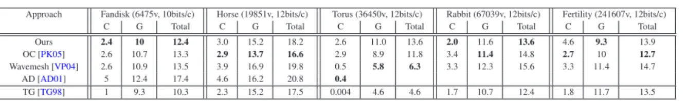
Table2shows lossless compression results for different reference models. All the models were quantized to 12 bits per coordinates, except for the fandisk model (quantized to 10 bits). Note that the different approaches do not have ex-actly equivalent quantization strategies. This results in small differences between the vertices coordinates of the recon-structed meshes with the three different approaches. Hence, the accuracy of this comparison is not maximal, albeit good enough to exhibit differences. For our coder, the connectivity bitstream consists in the set of midpoint codes, the incident flip codes used to decrease the connectivity drift and the edge flips codes used to reconstruct the exact input
connectiv-S. Valette, R. Chaine & R. Prost / Progressive Lossless Mesh Compression Via Incremental Parametric Refinement 9 Approach Fandisk (6475v, 10bits/c) Horse (19851v, 12bits/c) Torus (36450v, 12bits/c) Rabbit (67039v, 12bits/c) Fertility (241607v, 12bits/c)
C G Total C G Total C G Total C G Total C G Total
Ours 2.4 10 12.4 3.0 15.2 18.2 2.6 11.0 13.6 2.0 11.6 13.6 4.6 9.3 13.9
OC [PK05] 2.6 10.7 13.3 2.9 13.7 16.6 2.9 8.9 11.8 3.4 11.4 14.8 2.7 10 12.7
Wavemesh [VP04] 2.6 10.9 13.5 3.9 16.9 19.8 0.5 5.8 6.3 3.3 12.3 15.6 3.3 11.4 14.7 AD [AD01] 5 12.4 17.4 4.6 16.2 20.8 0.4
TG [TG98] 1 9.3 10.3 2.3 15.2 17.5 0.004 4.6 4.6 1.7 10.7 12.4 1.8 11.7 13.5
Table 2: Comparison of lossless compression efficiency between our approach and previous works. Numbers are in bits/vertex
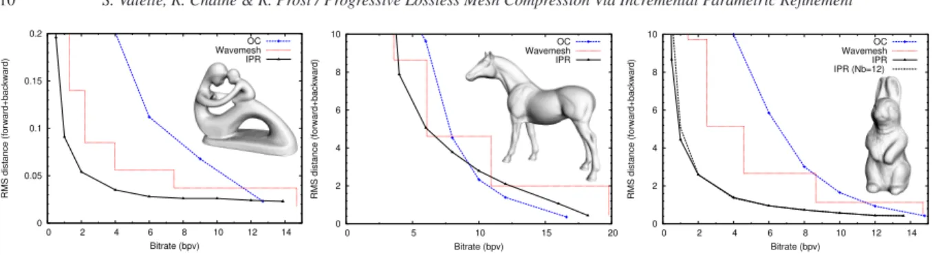
ity. The geometry bitstream consists in the delta-coordinates (decomposed into sign and amplitude codes) and the quanti-zation refinement bits. The cases where our approach did not outperform other coders are: (1) with the horse model, where the base mesh has 200 vertices, which causes a relatively high coding cost of about 0.9bpv for the base mesh, with our naive approach. But the transmission of the remaining geom-etry and topology is convincing, since its coding cost reduces to 17.3bpv. (2) with the torus model, which has very regu-lar connectivity and is then a very good fit for connectivity-driven approaches such as Wavemesh and the coder of Alliez & Desbrun [AD01]. (3) with the fertility model, due to the final edges flip sequence accounting for more than 50% of the connectivity bitstream. Figure9shows the rate-distortion curves obtained when performing progressive transmission for the Fertility model (left), the horse (middle) and the rab-bit (right), where the distortion is measured in terms of raw RMS distance (forward+backward) with METRO [CRS98]. As Wavemesh only provides a limited number of resolution levels, its distortion curve is represented by steps, where each step denotes an increase in resolution. For the rabbit and Fertility models, which are relatively simple models, our approach outperforms both Wavemesh and the OC coder. For the rabbit, we also provide the rate-distortion curve when using constant quantization (Nb= Qm= 12). It can be
no-ticed that adaptive quantization is beneficial at bitrates lower than 2bpv. The results on the horse model show that our ap-proach still performs very well at low bitrates, but is gradu-ally outperformed by the OC coder as the bitrate increases.
6. Discussion
In this paper, we have proposed a novel progressive lossless compression scheme, based on Incremental Parametric Re-finement, where the algorithm reconstructs visually pleasing meshes at a low coding cost by predicting the refinement lo-cations (i.e. the edge splits) and the required precision for each vertex. The remaining changes in the mesh connectiv-ity are performed automatically. Experimental results show that the concept behind IPR is of great interest for efficient progressive compression of 3D models, from small models of a few thousand vertices to models with a high sampling density. Our approach still leaves room for future improve-ments such as more fine-grained criteria (for the refinement location and for the balance between quantization and ver-tices density) and efficient coding of the delta-coordinates by introducing context-dependent coding schemes. Also,
studying non-inform refinement schemes seems an interest-ing perspective. Finally, findinterest-ing the always correct and op-timal vertex insertion strategy is a challenging problem, in-volving topology, geometry and information theory. Our ap-proach is currently a constant-topology scheme, but using non-constant-topology refinement operators such as gener-alized vertex splits at specific times during reconstruction could allow us to encode meshes with complex topology starting from very simple base meshes.
Acknowledgements
We thank the anonymous reviewers for their valuable com-ments which helped improving the quality of the paper. We also thank Arnaud Gelas for fruitful discussions on Delau-nay flips. The fertility model is courtesy of the Aim@Shape shape repository. Our implementation is based on the Visu-alization ToolKit (www.vtk.org).
References
[AD01] ALLIEZP., DESBRUNM.: Progressive encoding for loss-less transmission of 3d meshes. In ACM Siggraph Conference
Proceedings(2001), pp. 198–205.2,8,9
[AUGA07] ALLIEZP., UCELLIG., GOTSMANC., ATTENEM.: Recent advances in remeshing of surfaces. In Shape Analysis
and Structuring, de Floriani L., Spagnuolo M., (Eds.). Springer, 2007.2
[CGR07] CHAINE R., GANDOINP.-M., ROUDET C.: Mesh
Connectivity Compression Using Convection Reconstruction. In
ACM Symposium on Solid and Physical Modeling (ACM SPM)
(June 2007), Siggraph A., (Ed.), pp. 41–49.3
[COLR99] COHEN-ORD., LEVIND., REMEZO.: Progressive compression of arbitrary triangular meshes. In IEEE
Visualiza-tion 99(1999), pp. 67–72.2
[CRS98] CIGNONI P., ROCCHINI C., SCOPIGNO R.: Metro: Measuring error on simplified surfaces. Computer Graphics
Fo-rum 17, 2 (1998), 167–174.9
[Dee95] DEERINGM.: Geometry compression. In SIGGRAPH
’95: Proceedings of the 22nd annual conference on Computer graphics and interactive techniques(New York, NY, USA, 1995), ACM, pp. 13–20.1
[DZM07] DYERR., ZHANGH., MÖLLERT.: Delaunay mesh construction. In SGP ’07 (July 2007), Eurographics Association, pp. 273–282.4
[GD02] GANDOINP.-M., DEVILLERSO.: Progressive lossless compression of arbitrary simplicial complexes. In SIGGRAPH
’02: Proceedings of the 29th annual conference on Computer graphics and interactive techniques(New York, NY, USA, 2002), ACM, pp. 372–379.2,4
Figure 9: Comparison of rate-distortion efficiency on different models: fertility (left), horse (middle) and rabbit (right).
[GGH02] GUX., GORTLERS. J., HOPPEH.: Geometry im-ages. ACM Trans. Graph. (proceedings of SIGGRAPH 2002) 21, 3 (2002), 355–361.2
[GH97] GARLAND M., HECKBERT P. S.: Surface simplifi-cation using quadric error metrics. In SIGGRAPH ’97:
Pro-ceedings of the 24th annual conference on Computer graphics and interactive techniques(New York, NY, USA, 1997), ACM
Press/Addison-Wesley Publishing Co., pp. 209–216.7,8 [Got03] GOTSMANC.: On the optimality of valence-based
con-nectivity coding. Computer Graphics Forum 22 (March 2003), 99–102(4).1
[GUW01] GAOZ., URRUTIA J., WANG J.: Diagonal flips in labelled planar triangulations. Graphs Combin 17 (2001), 647– 657.6
[GVSS00] GUSKOV I., VIDIM ˇCE K., SWELDENS W.,
SCHRÖDER P.: Normal meshes. In SIGGRAPH ’00:
Pro-ceedings of the 27th annual conference on Computer graphics and interactive techniques(New York, NY, USA, 2000), ACM Press/Addison-Wesley Publishing Co., pp. 95–102.2
[Hop96] HOPPEH.: Progressive meshes. In ACM Siggraph 96
Conference Proceedings(1996), pp. 99–108.2
[ILS05] ISENBURGM., LINDSTROMP., SNOEYINKJ.: Lossless compression of predicted floatingpoint geometry. JCAD
-Journal for Computer-Aided Design 37(2005), 2005.2
[KBG02] KARNIZ., BOGOMJAKOVA., GOTSMANC.: Efficient compression and rendering of multi-resolution meshes. In VIS
’02: Proceedings of the conference on Visualization ’02 (Wash-ington, DC, USA, 2002), IEEE Computer Society, pp. 347–354. 2
[KG00] KARNI Z., GOTSMAN C.: Spectral Compression of Mesh Geometry. In ACM Siggraph 00 Conference Proceedings (2000), pp. 279–286.2
[Kob00] KOBBELTL.: √3-subdivision. In SIGGRAPH ’00:
Pro-ceedings of the 27th annual conference on Computer graphics and interactive techniques(New York, NY, USA, 2000), ACM
Press/Addison-Wesley Publishing Co., pp. 103–112.2 [KR99] KINGD., ROSSIGNACJ.: Optimal Bit Allocation in 3D
Compression. Journal of Computational Geometry, Theory and
Applications 14(1999), 91–118.3
[KSS00] KHODAKOVSKY A., SCHRÖDER P., SWELDENSW.:
Progressive Geometry Compression. ACM Siggraph Conference
Proceedings(2000), 271–278.2
[LCL∗06] LEWINER T., CRAIZERM., LOPESH., PESCO S., VELHOL., MEDEIROSE.: Gencode: geometry-driven compres-sion for general meshes. Computer Graphics Forum 25, 4 (de-cember 2006), 685–695.2
[LSS∗98] LEE A. W. F., SWELDENS W., SCHRÖDER P.,
COWSARL., DOBKIND.: Maps: multiresolution adaptive pa-rameterization of surfaces. In SIGGRAPH ’98: Proceedings of
the 25th annual conference on Computer graphics and interac-tive techniques(New York, NY, USA, 1998), ACM, pp. 95–104.
7
[PA05] PAYANF., ANTONINIM.: An efficient bit allocation for compressing normal meshes with an error-driven quantization.
Comput. Aided Geom. Des. 22, 5 (2005), 466–486.2
[PK05] PENGJ., KUOC.-C. J.: Geometry-guided progressive lossless 3d mesh coding with octree (ot) decomposition. ACM
Trans. Graph. 24, 3 (2005), 609–616.2,3,4,8,9
[PM05] PEYRÉG., MALLATS.: Surface compression with ge-ometric bandelets. In SIGGRAPH ’05: ACM SIGGRAPH 2005
Papers(New York, NY, USA, 2005), ACM, pp. 601–608.2 [PR00] PAJAROLA R., ROSSIGNAC J.: Compressed
Progres-sive Meshes. IEEE Transactions on Visualization and Computer
Graphics 6(1)(2000), 79–93.2
[PS06] POULALHOND., SCHAEFFER G.: Optimal coding and sampling of triangulations. Algorithmica 46, 3 (2006), 505–527. 1
[Ros99] ROSSIGNAC J.: EdgeBreaker : Connectivity Compres-sion for Triangle Meshes. IEEE Transactions on Visualization
and Computer Graphics(1999).1
[SAPH04] SCHREINERJ., ASIRVATHAMA., PRAUNE., HOPPE
H.: Inter-surface mapping. ACM Transactions on Graphics
(pro-ceedings of SIGGRAPH 2004) 23(2004), 870–877.7
[SP96] SAIDA., PEARLMANW.: A new, fast, and efficient im-age codec based on set partitioning in hierarchical trees. IEEE
Transactions on Circuits and Systems for Video Technology 6, 3
(June 1996), 243–250.3
[TG98] TOUMAC., GOTSMANC.: Triangle Mesh Compression.
Graphics Interface 98 Conference Proceedings(1998), 26–34.1, 8,9
[TGHL98] TAUBING., GUÉZIECA., HORNW., LAZARUSF.:
Progressive Forest Split Compression. In ACM Siggraph 98
Con-ference Proceedings(1998), pp. 123–132.2
[Tut62] TUTTEW.: A Census of Planar Triangulations. Canadian
Journal of Mathematics 14(1962), 21–38.1
[VP04] VALETTES., PROSTR.: A wavelet-based progressive compression scheme for triangle meshes : Wavemesh. IEEE
Trans Visu Comp Grap 10, 2 (2004), 123–129.2,8,9
[Wag36] WAGNERK.: Bemerkung zum vierfarbenproblem. Jber.