HAL Id: hal-01635468
https://hal.archives-ouvertes.fr/hal-01635468
Submitted on 15 Nov 2017
HAL is a multi-disciplinary open access
archive for the deposit and dissemination of
sci-entific research documents, whether they are
pub-lished or not. The documents may come from
teaching and research institutions in France or
abroad, or from public or private research centers.
L’archive ouverte pluridisciplinaire HAL, est
destinée au dépôt et à la diffusion de documents
scientifiques de niveau recherche, publiés ou non,
émanant des établissements d’enseignement et de
recherche français ou étrangers, des laboratoires
publics ou privés.
2-MANIFOLD RECONSTRUCTION FROM SPARSE
VISUAL FEATURES
Vadim Litvinov, Shuda Yu, Maxime Lhuillier
To cite this version:
Vadim Litvinov, Shuda Yu, Maxime Lhuillier. 2-MANIFOLD RECONSTRUCTION FROM SPARSE
VISUAL FEATURES. International Conference on 3D Imaging, Dec 2012, Liège, Belgium.
�hal-01635468�
2-MANIFOLD RECONSTRUCTION FROM SPARSE VISUAL FEATURES
Vadim Litvinov, Shuda Yu, and Maxime Lhuillier
Institut Pascal, UMR 6602 CNRS/UBP/IFMA, Campus des C´ezeaux, Aubi`ere, France
ABSTRACT
The majority of methods for the automatic surface recon-struction of a scene from an image sequence have two steps: Structure-from-Motion and dense stereo. From the complexity viewpoint, it would be interesting to avoid dense stereo and to generate a surface directly from the sparse features recon-structed by SfM. This paper adds two contributions to our previous work on 2-manifold surface reconstruction from a sparse SfM point cloud: we quantitatively evaluate our results on standard multiview dataset and we integrate the reconstruc-tion of image curves in the process.
Index Terms— 2-Manifold, Surface Reconstruction, 3D Delaunay Triangulation, Structure-from-Motion, Curves.
1. INTRODUCTION
The automatic surface reconstruction of a scene from an image sequence is still an active topic. First, we summarize the advan-tages of the previous work [17] which estimates a 2-manifold surface directly from the sparse cloud of 3D points recon-structed by Structure-from-Motion (SfM). Then, we present our contributions.
The input point cloud is sparse (not dense) since only interest points, such as Harris or SIFT, are reconstructed. This greatly reduces the complexity of a surface reconstruction from points, and this is interesting for the compact 3D modeling of large scenes such as cities. Furthermore, a surface estimated from a sparse SfM cloud (and its visibility information) can be used as the initialization for a dense stereo step [7], which deforms the surface such that the global photo-consistency is optimized (this improves the surface quality). The dense stereo step is outside the paper scope.
The output surface is a 2-manifold; this is in contrast to other surface reconstruction methods [8, 9, 13, 10] with the same sparse input. For memory, a surface is a 2-manifold if and only if every point in the surface has a surface neigh-borhood which is topologically a disk. Since our surface is triangulated, every triangle is exactly connected by its 3 edges to 3 different triangles, the surface has neither holes nor self-intersections, and it cuts the 3D space into inside and outside regions. The manifold property is used by a lot of computer
Thanks to CNRS, UBP, and Region of Auvergne for funding.
graphic methods [1] and dense stereo methods which enforce smoothness or curvature constraints on the surface (e.g. [2]). The contributions of the paper are the following: we add reconstructed curves to the input point cloud in [17], and we experiment on both multiview image data with ground truth [14, 15] and omnidirectional video image sequences (Ladybug). The work [4, 11, 16, 17] (including ours [17]) on 2-manifold reconstruction from sparse SfM data does not do that. Our curve reconstruction method involves matching based on correlation and assume that the epipolar constraint is known (this is different from curve reconstruction in [3] where the correlation is not used). Section 2 summarizes the surface reconstruction method and describes the curve reconstruction. Sections 3 and 4 are the experiments and the conclusion.
2. AUTOMATIC SCENE MODELING
Here we briefly summarize two steps: SfM (Section 2.1) and surface reconstruction from points and visibilities (Section 2.2). Then Section 2.3 describes the curve reconstruction.
2.1. Sparse SfM
Our SfM is similar to [12] in the central generic case (the cam-era is calibrated) and alternates the steps below. First, a new key-frame is selected from the input video and interest points are matched with the previous key-frame using correlation. The new key-frame is such that the number of its matches with the two previous key-frames is larger than a threshold. Then, the new pose is robustly estimated (using Grunert’s method [5] and RANSAC) and new 3D points are reconstructed from the new matches. Lastly, local bundle adjustment refines the geom-etry of the 3-most recent key-frames. The geomgeom-etry includes both points and camera poses.
2.2. Surface Reconstruction from Points and Visibilities This is the method in [17]. First, the 3D Delaunay triangu-lation T of the list P of reconstructed points is build: T par-titions the convex hull of P , and the circumsphere (sphere circumscribing tetrahedron) of every tetrahedron in T does not contain any vertex of T within it. Second, every tetrahedron in T is labeled either free-space or matter with the help of the rays provided by SfM. A ray is a line segment connecting
a 3D point to a viewpoint used to reconstruct it. A tetrahe-dron is free-space if it is intersected by a ray, otherwise it is matter. Third, the labeling is used to generate the surface. Several methods [13, 10, 9] directly consider the target surface as the list of triangles separating the free-space and matter. Unfortunately, the resulting surface can be non-manifold.
In order to generate a 2-manifold, a region-growing ap-proach is applied. The idea is to grow iteratively an outside region O in the free-space region by maintaining the man-ifold property on the border of O during the growing [17]. Before the growing, we assign inside to all tetrahedrons. The final manifold is the list of triangles separating the outside tetrahedrons and inside tetrahedrons.
Lastly, post-processing is used to improve the quality of the surface. It includes peak removal, surface denoising using discrete Laplacian, triangle removal in the sky (optional), and surface texturing.
2.3. Reconstruct and Integrate Curves
Here we reconstruct curves in 3D from image edges. The result is a list of sampled 3D points along the curves, which are added to the SfM points as inputs to the surface estimation. There are several steps: detection and matching in Section 2.3.1, reconstruction and sampling in Section 2.3.2.
2.3.1. Detection and Matching
First of all, the edge curves are detected in the incoming key-frame using the well known Canny operator. Then, they are parametrized in the horizontal or vertical direction (depending on the main curve orientation), refined using the gradient orien-tation information provided by Canny, and filtered to remove the curves that are too short for being useful.
Then the curves are matched with those in the previous key-frame. Unfortunately, curve geometry based matching method as described in [3] exhibited bad performance when the images contained a lot of condensed and similar curves (for example, as in the Ladybug datasets, see Section 3), it just can’t make a matching decision based on curve geometry alone. So, we decided to use a correlation based method heavily inspired by a classical points matching.
To perform a curve matching between images I1and I2
we proceed as follow: for each curve C1in I1we construct
an epipolar lines strip in the image I2, then we reject all the
curves not at least partially included into it. The remaining curves of I2form a list of candidates Lc. For each curve C2in
Lcwe compute a zero-normalized cross-correlations (ZNCC)
between intersections of C2 with the epipolar lines and the
points of C1that produced them. Finally, the mean value of
all these correlations define the score of the curve C2. C1is
matched with the curve of Lchaving the best score.
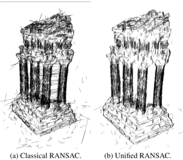
(a) Classical RANSAC. (b) Unified RANSAC.
Fig. 1. Different 3D curve initialization methods.
2.3.2. Reconstruction and Sampling
First, the lists of curve tracks generated in Section 2.3.1 are converted to lists of image point tracks thanks to the epipo-lar constraints. A curve track is a list of matched curves ci0, ci0+1, ...ci1such that ciis in the i-th key-frame. A point
track is a list of matched points pi0, pi0+1, ...pi1where piis in
the i-th key-frame: pi+1is obtained from piby the intersection
of ci+1and the epipolar line of piin the i + 1-image. If the
angle between the epipolar line and the ci+1tangent at pi+1
is small, the intersection is inaccurate and the point track is truncated (a point track can be shorter than the curve track).
Then, every point track is reconstructed by ray intersection: RANSAC is used for robustness and initializing a Levenberg-Marquardt optimization [6]. Unfortunately, using this direct approach leads to some strange artifacts (left of Fig. 1 for “Temple” [14] dataset). In fact, all the points of the same curve do not necessarily use the same views to initialize themselves by RANSAC. This difference in initial position leads to zigzag like 3D curves. To avoid this problem, we perform a two-step initialization: first, all the points are initialized independently; then, at the second stage, we select the two views that were used the most often and all the points are initialized using these two views. As can be seen on the right image of Fig. 1, this approach greatly improves the reconstructed curves.
Finally, we only retain for surface estimation one recon-structed point over s points for every curve track. The step size s is large enough to preserve speed and sparsity of the global algorithm and at the same time small enough to ensure that curves are correctly integrated into the Delaunay triangulation.
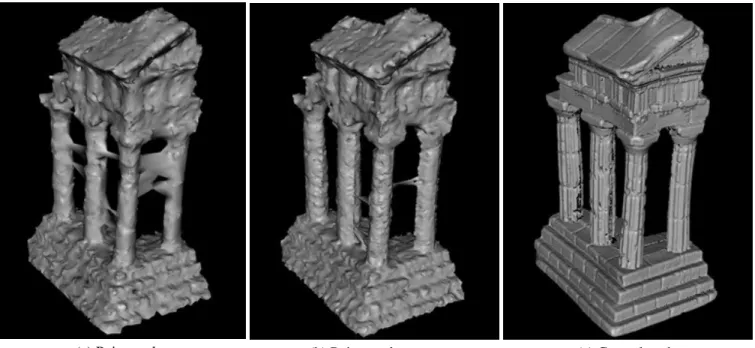
(a) Points only. (b) Points and curves. (c) Ground truth.
Fig. 2. “Temple” dataset reconstruction results.
3. EXPERIMENTS
Our method is evaluated on three different datasets: “Temple” dataset [14], “Fountain-P11” and “Herzjesu-P8” dataset [15], and finally our own “Hall” and “Aubi`ere” dataset. The first two are provided with the ground truth so this allows us to quantitatively evaluate the performance of our algorithm and to compare it with the others. The third allows us to qualitatively evaluate our method on a cluttered interior and a residential scene. All the processing times are evaluated on a 4xIntel Xeon W3530 at 2.8 GHz. A summary of important values about every dataset presented in this section can be found in table 1.
Note that our method was initially designed for the re-construction of complete environments using omnidirectional cameras as in our own (third) dataset. In this case, the camera positions are assumed to be inside the convex hull of the re-constructed scene points. In the other cases (first and second datasets) a workaround is needed: we add Steiner vertices (ex-tra points) at the border of a large bounding box of the object (“Temple”) or behind the camera (“Fountain-Herzjesu”) to the Delaunay triangulation, then we apply our method and remove the triangles which are incident to these Steiner vertices.
3.1. “Temple” dataset
The “Temple” provided by [14] is a standard multiview recon-struction dataset (312 separate views). In this evaluation, we use the camera positions provided with the dataset to recon-struct the 3D points.
Two models were sent for evaluation to the dataset creators. The first (see Fig. 2.a) is reconstructed using the points only and the second one (see Fig. 2.b) is reconstructed using points and curves. The ground truth image is provided for reference on Fig. 2.c. The point-only model is reconstructed in 31 s. and provides an accuracy of 0.66 mm. (for 90% of reconstructed points) and completeness of 93% (for 1.25 mm. error). The points and curves reconstruction takes 59 s. and provides an accuracy of 0.59 mm. and completeness of 95.4%. (These values can be compared to those of other algorithms at the following address:http://vision.middlebury.edu/ mview/eval/).
This lead us to two conclusions. Firstly, the use of the curves provides indeed an enhancement to the resulting model. Secondly, compared to other methods evaluated using the same datasets, our algorithm is, from the best of our knowledge, the fastest CPU based reconstruction method, and the resulting precision is not so bad compared to majority of the dense stereo algorithms. This makes our method a good candidate for initialization of a dense stereo method.
3.2. “Fountain-P11” and “Herzjesu-P8” datasets
“Fountain” and “Herzjesu” are another standard set of mul-tiview stereo datasets provided with their respective ground truths (courtesy of [15]). They contain, respectively, 11 and 8 high-resolution images. In this evaluation, we use the cam-era positions provided with the dataset to reconstruct the 3D points.
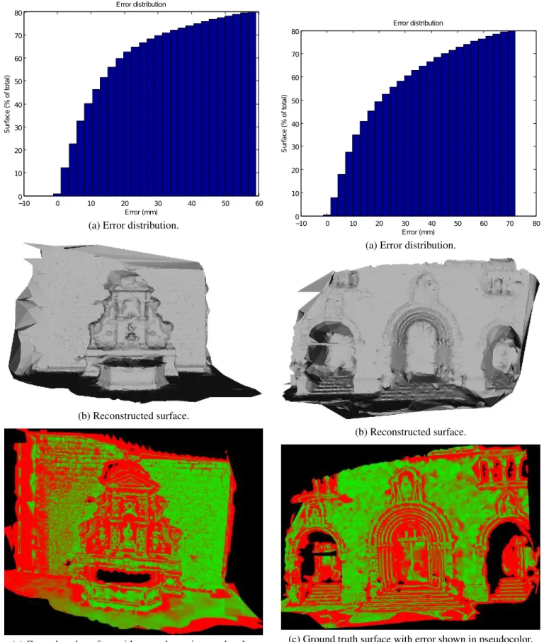
−10 0 10 20 30 40 50 60 0 10 20 30 40 50 60 70 80 Error distribution Error (mm) S ur fa ce (% of to ta l)
(a) Error distribution.
(b) Reconstructed surface.
(c) Ground truth surface with error shown in pseudocolor. Fig. 3. “Fountain” dataset reconstruction results.
−10 0 10 20 30 40 50 60 70 80 0 10 20 30 40 50 60 70 80 Error distribution Error (mm) S ur fa ce (% of to ta l)
(a) Error distribution.
(b) Reconstructed surface.
(c) Ground truth surface with error shown in pseudocolor. Fig. 4. “Herzjesu” dataset reconstruction results.
we subdivide our output mesh with a very thin step and, for each points of the output mesh, we calculate the distance to the nearest point of the ground truth mesh.
The results can be seen on Figs. 3 and 4 respectively. Part (a) provides an error distribution cumulative histogram. Part (b) shows the output mesh and part (c) displays the estimated model colored in function of the error value (green is better, scaled between values at 20% and 80% for better visibility). The computations of “Fountain” and “Herzjesu” take 123 s. and 74 s., respectively.
As can be seen, our method provides honorable results, so it can be a good choice when the speed of computation is at least as important as precision. We do not show the results obtained by mixing points with curves because adding curves provides a very minor improvement.
3.3. “Hall” and “Aubi`ere” datasets
(a) “Hall”.
(b) “Aubi`ere”.
Fig. 5. Ladybug images for “Hall” and “Aubi`ere” video se-quences.
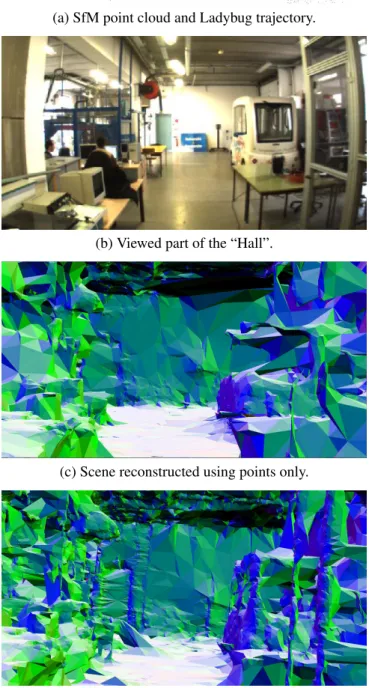
“Hall” and “Aubi`ere” datasets are two large datasets taken in and in the proximity of Institut Pascal with a PointGrey Ladybug omnidirectional camera. Ladybug is a rigid multi-camera system consisting of six synchronized multi-cameras each of which takes 1024x768 images at 15 frames/second. Unfor-tunately, ground truth is not available for these acquisitions, so we provide only qualitative results. This allows us to eval-uate the general performance of the complete algorithm as described in the Section 2. Fig. 5 shows the complete Ladybug frames for both sequences.
“Hall” sequence is roughly 20 m. long and contains 1211 frames (6 images each). There are 117 selected key-frames; the total processing time is about 19 min. including curves (the main computation part is due to SfM). Reconstruction of the representative scene can be seen on Fig. 6: part (b) contains a real image of the scene for reference. We see that mixing points and curves provides a better result than the usage of the points alone.
“Aubi`ere” sequence is around 700 m. long and contains 3140 frames. There are 655 selected key-frames and the total
(a) SfM point cloud and Ladybug trajectory.
(b) Viewed part of the “Hall”.
(c) Scene reconstructed using points only.
(d) Scene reconstructed using points and curves.
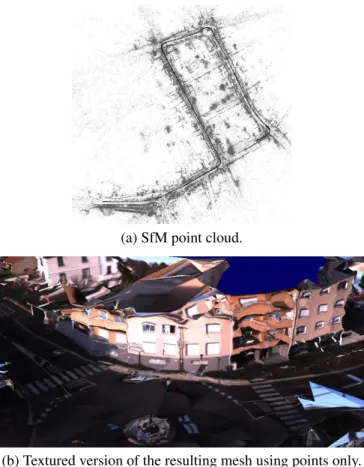
(a) SfM point cloud.
(b) Textured version of the resulting mesh using points only.
(c) Resulting mesh using points only.
(d) Resulting mesh using points and curves.
Fig. 7. “Aubi`ere” dataset reconstruction results.
processing time is about 56 min. (the main computation part is due to SfM). The results are on Fig. 7. Contrary to the previous sequence, the curves doesn’t bring any significant improvement over the points alone. Global views without curves are also shown in Fig. 8;
4. CONCLUSION
The contributions of this paper are (1) the evaluation of the 2-manifold surface sparse reconstruction method described in [17] against ground truth in some common multiview stereo datasets and (2) the evaluation of the enhancement provided by mixing the input points cloud of this algorithm with recon-structed curves.
According to the comparison of the output surface with the ground truth, the precision achieved by this method cannot yet compete with the dense stereo methods, but we think that it is sufficient to be used as initialization of dense stereo. Further-more, given the achieved speed, the algorithm is indeed a good choice not only for this purpose but also for the applications where the speed is at least as important as the precision.
On the other hand, mixing the curves with the points of interest provides some significant enhancement if input images are only slightly textured as in “Temple” and “Hall”. But it is of little interest in the textured case, as for “Fountain” and “Herzjesu”. So there are no general conclusion and the real benefits must be evaluated for each sequence individually. Nev-ertheless, it will be interesting to perform more investigations in this matter as better results can certainly be achieved.
5. REFERENCES
[1] M. Botsch, L. Kobbelt, M. Pauly, P. Alliez, and B. Levy. Polygon Mesh Processing. AK Peters, 2010.
[2] C.H. Esteban and F. Schmitt. Silhouette and Stereo Fu-sion 3D Object Modeling. Computer ViFu-sion and Image Understanding, 96:367–392, 2004.
[3] R. Fabbri and B. Kimia. 3D Curve Sketch: Flexible Curve-Based Stereo Reconstruction and Calibration. In the Conference on Computer Vision and Pattern Recog-nition (CVPR). IEEE, 2010.
[4] O. Faugeras, E. Le Bras-Mehlman, and J.D. Boissonnat. Representing Stereo Data with the Delaunay Triangula-tion. Artificial Intelligence, pages 41–47, 1990.
[5] R. Haralick, C. Lee, K. Ottenberg, and M. Nolle. Review and analysis of solutions of the three point perspective pose estimation problem. International Journal of Com-puter Vision, 13(3):331–356, 1994.
[6] R. Hartley and A. Zisserman. Multiple View Geometry in Computer Vision. Cambridge University Press, 2003.
(a) Triangle normals.
(b) Texturing.
(c) Triangle normals. (d) Texturing.
Temple Fountain-P11 Herzjesu-P8 Hall Aubi`ere Image resolution 1x640x480 1x3072x2048 1x3072x2048 6x1024x768 6x1024x768 Key-frames (total frames) 312 (312) 11 (11) 8 (8) 117 (1211) 493 (2443)
Harris points per frame 1.5k 60k 50k 24k 24k curve sampling size s 4 8 8 8 8 SfM 3D Points (curves) 32k (56k) 67k 29k 86k (145k) 295k (374k) Final triangles (curves) 49k (82k) 121k 52k 83k (305k) 399k (520k) Time: 3D points (+curves) 13 s. (+28 s.) 100 s. 64 s. 17 min. (+102 s.) 55 min. (+8 min.)
Time: Surface 18 s. 23 s. 10 s. 47 s. 81 s. Table 1. Descriptions of datasets used in our experimental tests (1k=1000).
[7] V. Hiep, K. Keriven, P. Labatut, and J.P. Pons. Towards High-Resolution Large-Scale Multi-View Stereo. In the Conference on Computer Vision and Pattern Recognition (CVPR). IEEE, 2009.
[8] A. Hilton. Scene Modeling from Sparse 3D Data. Image and Vision Computing, 23:900–920, 2005.
[9] P. Labatut, J.P. Pons, and K. Keriven. Efficient Multi-View Reconstruction of Large-Scale Scenes using Inter-est Points, Delaunay Triangulation and Graph-Cut. In the Conference on Computer Vision and Pattern Recognition (CVPR). IEEE, 2007.
[10] D. Lovi, N. Birkbeck, D. Cobzas, and M. Jagersand. Incremental Free-Space Carving for Real-Time 3D-Reconstruction. In International Symposium on 3D Data Processing, Visualization and Transmission (3DPVT), 2010.
[11] D. Morris and T. Kanade. Image Consistent Surface Triangulation. In the Conference on Computer Vision and Pattern Recognition (CVPR), 2000.
[12] E. Mouragnon, M. Lhuillier, M. Dhome, F. Dekeyser, and P. Sayd. Generic and Real-Time Structure-From-Motion using Local Bundle Adjustment. Image And Vision Computing (IVC), 27:1178–1193, 2009.
[13] Q. Pan, G. Reitmayr, and T. Drummond. ProFORMA: Probabilistic Feature-Based On-Line Rapid Model Ac-quisition. In British Machine Vision Conference (BMVC), 2009.
[14] S.M. Seitz, B. Curless, J. Diebel, D. Scharstein, and R. Szeliski. A Comparison and Evaluation of Multi-View Stereo Reconstruction Algorithms. In the Conference on Computer Vision and Pattern Recognition (CVPR). IEEE, 2006.
[15] C. Strecha, W. von Hansen, L. van Gool, P. Fua, and U. Thoennessen. On Benchmarking Camera Calibration and Multi-View Stereo for High Resolution Imagery. In the Conference on Computer Vision and Pattern Recog-nition (CVPR). IEEE, 2008.
[16] C.J. Taylor. Surface Reconstruction from Feature-Based Stereo. In the International Conference on Computer Vision (ICCV), 2003.
[17] S. Yu and M. Lhuillier. Surface Reconstruction of Scenes using a Catadioptric Camera. In the Conference on Com-puter Vision/ComCom-puter Graphics Collaboration Tech-niques and Application (MIRAGE). IEEE, 2011.