Morphometry of anatomical shape complexes with dense deformations and sparse parameters

HAL Id: hal-01015771

https://hal.inria.fr/hal-01015771

Submitted on 27 Jun 2014

HAL is a multi-disciplinary open access

archive for the deposit and dissemination of

sci-entific research documents, whether they are

pub-lished or not. The documents may come from

teaching and research institutions in France or

abroad, or from public or private research centers.

L’archive ouverte pluridisciplinaire HAL, est

destinée au dépôt et à la diffusion de documents

scientifiques de niveau recherche, publiés ou non,

émanant des établissements d’enseignement et de

recherche français ou étrangers, des laboratoires

publics ou privés.

Morphometry of anatomical shape complexes with dense

deformations and sparse parameters

Stanley Durrleman, Marcel Prastawa, Nicolas Charon, Julie R Korenberg, S.

Joshi, Guido Gerig, Alain Trouvé

To cite this version:

Stanley Durrleman, Marcel Prastawa, Nicolas Charon, Julie R Korenberg, S. Joshi, et al..

Morphom-etry of anatomical shape complexes with dense deformations and sparse parameters. NeuroImage,

Elsevier, 2014, �10.1016/j.neuroimage.2014.06.043�. �hal-01015771�

Morphometry of anatomical shape complexes with dense deformations and sparse

parameters

Stanley Durrlemana,b,c,d,e_{, Marcel Prastawa}f_{, Nicolas Charon}g_{, Julie R. Korenberg}h_{, Sarang Joshi}f_{, Guido Gerig}f_{, Alain Trouv´e}g

a_{INRIA, project-team Aramis, Centre Paris-Rocquencourt, France} b_{Sorbonne Universit´es, UPMC Universit´e Paris 06, UMR S 1127, ICM, Paris, France}

c_{Inserm, U1127, ICM, Paris, France} d_{CNRS, UMR 7225, ICM, Paris, France}

e_{Institut du Cerveau et de la Mo¨elle ´epini`ere (ICM), Hˆopital de la Piti´e Salpˆetri`ere, 75013 Paris, France} f_{Scientific Computing and Imaging (SCI) Institute, University of Utah, Salt Lake City, UT 84112, USA} g_{Centre de Math´ematiques et Leurs Applications (CMLA), Ecole Normale Sup´erieure de Cachan, 94230 Cachan, France}

h_{Brain Institute, University of Utah, Salt Lake City, UT 84112, USA}

Abstract

We propose a generic method for the statistical analysis of collections of anatomical shape complexes, namely sets of surfaces that were previously segmented and labeled in a group of subjects. The method estimates an anatomical model, the template

complex, that is representative of the population under study. Its shape reflects anatomical invariants within the dataset. In addition, the method automatically places control points near the most variable parts of the template complex. Vectors attached to these points are parameters of deformations of the ambient 3D space. These deformations warp the template to each subject’s complex in a way that preserves the organization of the anatomical structures. Multivariate statistical analysis is applied to these deformation parameters to test for group differences. Results of the statistical analysis are then expressed in terms of deformation patterns of the template complex, and can be visualized and interpreted. The user needs only to specify the topology of the template complex and the number of control points. The method then automatically estimates the shape of the template complex, the optimal position of control points and deformation parameters. The proposed approach is completely generic with respect to any type of application and well adapted to efficient use in clinical studies, in that it does not require point correspondence across surfaces and is robust to mesh imperfections such as holes, spikes, inconsistent orientation or irregular meshing.

The approach is illustrated with a neuroimaging study of Down syndrome (DS). Results demonstrate that the complex of deep brain structures shows a statistically significant shape difference between control and DS subjects. The deformation-based modeling is able to classify subjects with very high specificity and sensitivity, thus showing important generalization capability even given a low sample size. We show that results remain significant even if the number of control points, and hence the dimension of variables in the statistical model, are drastically reduced. The analysis may even suggest that parsimonious models have an increased statistical performance.

The method has been implemented in the software Deformetrica, which is publicly available at www.deformetrica.org.

Keywords: morphometry, deformation, varifold, anatomy, shape, statistics

1. Introduction

Non-invasive imaging methods such as Magnetic Resonance Imaging (MRI) enable analysis of anatomical phenotypic vari-ations over large clinical data collections. For example, MRI is used to reveal and quantify effects of pathologies on anatomy, such as hippocampal atrophy in neurodegenerative diseases or change in neuronal connectivity in neurodevelopmental disor-ders. Subject-specific digital anatomical models are built from the segmentation and labeling of structures of interest in im-ages. In neuroanatomy, these structures of interest are often volumes whose boundaries take the form of 3D surfaces. For a given individual, the set of such labeled surfaces, which we call an anatomical complex, is indicative of the shape of different brain objects and their relative position. Our goal is to per-form statistics on a series of such anatomical complexes from

subjects within a given population. We assume that the com-plex contains the same anatomical structures in each subject, so that interindividual differences are not due to the presence or absence of a structure or a split of one structure into two. The quantification of phenotypic variations across individuals or populations is crucial to find the anatomical substrate of neu-rologic diseases, for example to find an early biomarker of dis-ease onset or to correlate phenotypes with functional or geno-typic variables. Not only the quantification, but also the

de-scriptionof the significant anatomical differences are important in order to interpret the findings and drive the search for biolog-ical pathways leading to pathologies.

The core problem is the construction of a computational model for such shape complexes that would allow us to mea-sure differences between them and to analyze the distribution across a series of complexes. Geometric morphometric

meth-ods make use of the relative position of carefully defined ho-mologous points on surfaces, called landmarks (Bookstein, 1991; Dryden and Mardia, 1998). Landmark-free methods of-ten use geometric characteristics of the surfaces. They there-fore need to make strong assumptions about the topology of the surface, for example limiting analysis to genus zero sur-faces (Chung et al., 2003; Boyer et al., 2010) or using medial representations (Styner et al., 2005; Bouix et al., 2005; Gorc-zowski et al., 2010) or Laplace-Beltrami eigenfunctions (Reuter et al., 2006). Such methods can rarely be applied to raw sur-face meshes resulting from segmentation algorithms since such meshes may include small holes, show irregular sampling or split objects into different parts.

More important, such methods analyze the intrinsic shape of each structure independently, therefore neglecting the fact that brain anatomy consist of an intricate arrangement of various structures with strong interrelationships. By contrast, we aim at measuring differences between shape complexes in a way that can account for both the differences in shape of the individual components and the relative position of the components within the complex. This goal cannot be achieved by concatenating the shape parameters of each component or by finding correlations between such parameters (Tsai et al., 2003; Gorczowski et al., 2010), as such approaches do not take into account the fact that the organization of the shape complex would not change, and in particular, that different structures must not intersect.

One way to address this problem is to consider surfaces as embedded in 3D space and to measure shape variations induced by deformations of the underlying 3D space. This idea stems from Grenanders group theory for modeling objects (Grenan-der, 1994), which revisits morphometry by the use of 3D space deformations. The similarity between shape complexes is then quantified by the “amount” of deformation needed to warp one shape complex to another. Only smooth and invertible 3D de-formations (i.e., diffeomorphisms) are used, so that the internal organization of the shape complex is preserved during deforma-tion since neither surface intersecdeforma-tion nor shearing may occur. The approach determines point correspondences over the whole 3D volume by using the fact that surfaces should match as a soft constraint. The method is therefore robust to segmentation errors in that exact correspondences among points lying on sur-faces are not enforced. In this context, a diffeomorphism could be seen as a low-pass filter to smooth shape differences. In this paper, it is our goal to show that the deformation parameters capture the most relevant parts of the shape variations, namely the ones that would distinguish between normal and disease.

Here, we propose a method that builds on the implementa-tion of Grenanders theory in the LDDMM framework (Miller et al., 2006; Vaillant et al., 2007; McLachlan and Marsland, 2007). The method has 3 components: (i) estimation of an average model of the shape complex, called the template com-plex, which is representative of the population under study; (ii) estimation of the 3D deformations that map the template com-plex to the comcom-plex of each subject; and (iii) statistical analysis of the deformation parameters and their interpretation in terms of variations of the template complex. The first two steps are estimated simultaneously in a combined optimization

frame-work. The resulting template complex and set of deformations are now referred to as an atlas.

Previous attempts to estimate template shapes in this frame-work offered little control over the topology of the template, whether it consists in the superimposition of a multitude of sur-face sheets (Glaun`es and Joshi, 2006) or a set of unconnected triangles (Durrleman et al., 2009). The topology of the tem-plate may be chosen as one of a given subject’s complex (Ma et al., 2008), but this topology then inherits the mesh imperfec-tions that result from an individual segmentation. In this paper, we follow the approach initially suggested by Durrleman et al. (2012), which leaves the choice of the topology of the template with number of connected components to the user. This method estimates the optimal position of the vertices so that the shape of the template complex is an average of the subjects complexes. Here, we extend this approach in order to guarantee that no self-intersection could occur during the optimization.

The set of deformations that result from warping the tem-plate complex to each subjects complex captures the variabil-ity across subjects. The deformation parameters quantify how the subjects anatomy is different from the template, and can be used in a statistical analysis in the same spirit as in Vail-lant et al. (2004) and Pennec (2006). We follow the approach initiated in Durrleman et al. (2011, 2013), which uses control points to parameterize deformations. The number of control points is fixed by the user, and the method automatically adjusts their position near the most variable parts of the shape complex. The method therefore offers control over the dimension of the shape descriptor that is used in statistics, and thus avoids an unconstrained increase with the number of surfaces and their samplings (Vaillant and Glaun`es, 2005). We show that statis-tical performance is not reduced by this finite-dimensional ap-proximation and that the parameters can robustly detect subtle anatomical differences in a typical low sample size study. We postulate that in some scenarios, the statistical performance can even be increased, as the ratio between the number of subjects and the number of parameters becomes more favorable.

An important key element of the method is a similarity metric between pairs of surfaces. Such a metric is needed to optimize the deformation parameters that enable the best matching be-tween shape complexes. We use the varifold metric that has been recently introduced in Charon and Trouv´e (2013). It ex-tends the metric on currents (Vaillant and Glaun`es, 2005) in that it considers the non-oriented normals of a surface instead of the oriented normals. The method is therefore robust to pos-sible inconsistent orientation of the meshes. It also prevents the “canceling effect” of currents, which occurs if two surface ele-ments with opposite orientation face each other, and which may cause the template surface to fold during optimization. Other-wise, the metric inherits the same properties as currents: it does not require point-correspondence between surfaces and is ro-bust to mesh imperfections such as holes, spikes or irregular meshing (Vaillant and Glaun`es, 2005; Durrleman et al., 2009).

This paper is structured as follows to give a self-contained presentation of the methodology and results. We first focus on the main steps of the atlas construction, while discussing the technical details of the theoretical derivations in the appendices.

We then present an application to neuroimage data of a Down syndrome brain morphology study. This part focuses on the new statistical analysis of deformations that becomes possible with the proposed framework, and it also presents visual rep-resentations that may support interpretation and findings in the context of the driving clinical problem. The analysis also in-cludes an assessment of the robustness of the method in various settings.

2. Mathematical Framework

2.1. Kernel formulation of splines

In the spline framework, 3D deformations φ are of the form φ(x) = x + v(x), where v(x) is the displacement of any point x in the ambient 3D space, which is assumed to be the sum of radial basis functions K located at control point positions{ck}k=1,...,Ncp:

v(x) =

Ncp

X

k=1

K(x, ck)↵k. (1)

Parameters ↵1, . . . , ↵Ncp are vector weights, Ncpthe number of

control points and K(x, y) is a scalar function that takes any pair of points (x, y) as inputs. In the applications, we will use the Gaussian kernel K(x, y) = exp(_{− |x − y|}2/σ2

V), although other

choices are possible such as the Cauchy kernel K(x, y) = 1/(1 + |x − y|2/σ2

V) for instance.

It is beneficial to assume that K is a positive definite symmet-ric kernel, namely that K is continuous and that for any finite set of distinct points_{ci}iand vectors{↵i}i:

X

i

X

j

K(ci, cj)↵iT↵j≥ 0, (2)

the equality holding only if all ↵ivanish. Translation invariant

kernels are of particular interest. According to Bochner’s theo-rem, functions of the form K(x_{− y) are positive definite kernels} if and only if their Fourier transform is a positive definite op-erator, in which case (2) becomes a discrete convolution. This theorem enables an easy check if the previous Gaussian func-tion is indeed a positive-definite kernel, among other possible choices.

Assuming K is a kernel allows us to define the pre-Hilbert space V as the set of any finite sums of terms K(., c)↵ for vector weights ↵. Given two vector fields v1 =PiK(., ci)↵iand v2 =

P

jK(., c0j)βj, (2) ensures that the bilinear map

hv1, v2iV = X i X j K(ci, c0j)↵iTβj (3)

defines an inner-product on V. This expression also shows that any vector field v2 V satisfies the reproducing property:

hv, K(., c)↵iV = v(c)T↵, (4)

defined for any point c and weight ↵. The space of vector fields V could be “completed” into a Hilbert space by con-sidering possible infinite sums of terms K(., c)↵, for which (4)

still holds. Such spaces are called Reproducing Kernel Hilbert Spaces (RKHS) (Zeidler, 1991).

Using matrix notations, we denote c and α (resp. c0and β) in R3N

(resp. R3M) the concatenation of the 3D vectors ciand ↵i

(resp. c0

jand βj), so that the dot product (3) writeshv1, v2iV =

αT_{K(c, c0)β, where K(c, c0) is the 3N}

⇥ 3M matrix with entries

K(ci, c0_j)I3_⇥3.

2.2. Flows of diffeomorphisms

The main drawback of such deformations is their non-invertibility, as soon as the magnitude of v(x) or its Jacobian is “too” large. The idea to build diffeomorphisms is to use the vector field v as an instantaneous velocity field instead of a dis-placement field. To this end, we make the control points ck

and weights ↵kto depend on a “time” t that plays the role of a

variable of integration. Therefore, the velocity field at any time

t_{2 [0, 1] and space location x is written as:} vt(x) = Ncp X k=1 K(x, ck(t))↵k(t) (5) for all t_{2 [0, 1]}

A particle that is located at x0 at t = 0 follows the integral

curve of the following differential equation:

dx(t)

dt = vt(x(t)), x(0) = x0, (6)

This equation of motion also applies for control points. Using matrix notations, their trajectories follow the integral curves of ˙c(t) = K(c(t), c(t))α(t), c(0) = c0. (7)

At this stage, point trajectories are entirely determined by time-varying vector weights ↵k(t) and initial positions of control

points c0.

For each time t, one may consider the mapping x0 ! φt(x0),

where φt(x0) is the position at time t of the particle that was at

x0 at time t = 0, namely the solution of (6). At time t = 0,

φ0=IdR3(i.e., φ₀(x₀) = x₀). At any later time t, the mapping is

a 3D diffeomorphism. Indeed, it is shown in Miller et al. (2006) that (6) has a solution for all time t > 0, provided that time-varying vectors ↵k(t) are square integrable. It is also shown

that these mappings are smooth, invertible and with smooth in-verse. In particular, particles cannot collide, thus preventing self-intersection of shapes. At any space location x, one can find a particle that passes by this point at time t via backward integration, thus preventing shearing or tearing of the shapes embedded in the ambient space.

For a fixed set of initial control points c0, the time-varying

vectors α(t) define a path (φt)tin a certain group of

diffeomor-phisms, which starts at the identity φ0 =Id_R3, and ends at φ1,

the latter representing the deformation of interest. We aim to es-timate such a path, so that the mapping φ1 brings the template

shapes as close as possible to the shapes of a given subject. The problem is that the vectors, which enable us to reach a given φ1from the identity, are not unique. It is natural to choose the

vectors that minimize the integral of the kinetic energy along the path, namely

1 2 Z 1 0 kv tk2Vdt = 1 2 Z 1 0 α(t)TK(c(t), c(t))α(t)dt. (8) We show in Appendix A that the minimizing vectors α(t), con-sidering c(0) and c(1) fixed, satisfy a set of differential equa-tions. Together with the equations driving motion of control points (7), they are written as:

8 > > > > > > > > > > < > > > > > > > > > > : ˙ck(t) = Ncp X p=1 K(ck(t), cp(t))↵p(t) ˙ ↵k(t) =− Ncp X p=1 ↵k(t)T↵p(t)r1K(ck(t), cp(t)) (9) Denoting S(t) = c(t) α(t) !

the state of the system of control points at time t, (9) could be written in short as

˙S(t) = F(S(t)), S(0) = c0 α0

!

. (10)

The flow of deformations is now entirely parameterized by initial positions of control points c0 and initial vectors α0

(called momenta in this context). Integration of (10) computes the position of control points c(t) and momenta α(t) at any time

t from initial conditions. Control points and momenta define, in turn, a time-varying velocity field vtvia (5). Any

configura-tion of points in the ambient space, concatenated into a single vector X0, follows the trajectory X(t) that results from the

in-tegration of (6). Using matrix notation, this ODE is written as ˙

X(t) = vt(X(t)) = K(X(t), c(t))α(t) with X(0) = X0, which can

be further shortened to: ˙

X(t) = G(X(t), S(t)), X(0) = X0 (11)

A given set of initial control points c0 defines a sub-group

of finite dimension of our group of diffeomorphisms. Paths of minimal energy, also called geodesic paths, are parameterized by initial momenta α0, which play the role of the logarithm

of the deformation φ1 in a Riemannian framework.

Integra-tion of (10) computes the exponential map. It is easy to check that_kvtkV is constant along such geodesic paths. Therefore, the

length of the geodesic path that connects φ0 =Id_R3 to φ1(i.e.,

R1

0 kvtkVdt) simply equals the norm of the initial velocity (i.e.,

kv0kV).

2.3. Varifold metric between surfaces

Deformation parameters c0, α0 will be estimated so as to

minimize a criterion measuring the similarity between shape complexes. To this end, we define a distance between sur-face meshes in this section, and show how to use it for shape complexes in the next section. If the vertices in two meshes correspond, then the sum of squared differences between ver-tex positions could be used. However, finding such correspon-dences is a tedious task and is usually done by deforming an

atlas to the meshes. This procedure leads to a circular defini-tion, since we need this distance to find deformations between meshes! Among distances that are not based on point corre-spondences, we will use the distance on varifolds (Charon and Trouv´e, 2013). In the varifold framework, meshes are embed-ded into a Hilbert space in which algebraic operations and dis-tances are defined. In particular, the union of meshes translates to addition of varifolds. The inner-product between two meshes S and S0is given as:

⌦S, S0↵ W⇤ = X p X q KW(cp, c0q) ⇣ nT pn0q ⌘2 / / /np / / / / / /n0q / / / (12) where cpand np(resp. c0qand n0q) denotes the centers and

nor-mals of the faces of_{S (resp. S}0). The norm of the normals// /np

/ / / equals the area of the mesh cell. KW _{is a kernel, typically a}

Gaussian function with a fixed width σW.

The distance between S and S0 _{then simply writes:}

dW(S, S0)2 =kS − S0k2W⇤ =hS, SiW⇤+hS0,S0iW⇤− 2 hS, S0iW⇤.

One notices that the inner-product, and hence the distance, does not require vertex correspondences. The distance measures shape differences in the difference in normals directions, by considering every pair of normals in a neighborhood of size σW.

It considers meshes as a cloud of undirected normals and there-fore does not make any assumptions about the topology of the meshes; one mesh may consist of several surface sheets, have small holes or have irregular meshing. Differences in shape at a scale smaller than the kernel width σWare smoothed, thus

mak-ing the distance robust to spikes or noise that may occur durmak-ing image segmentation. The inner-product resembles the one in the currents framework (Vaillant and Glaun`es, 2005; Durrleman et al., 2009), except that(nTpn0q)

2 |np||n0q| now replaces ⇣ nTpn0q ⌘ . With this new expression, the distance is invariant if some normals are flipped. It does not require the meshes to have a consistent ori-entation. Contrary to other correspondence-free distance such as the Hausdorff distance, the gradient of this distance with re-spect to the vertex positions is easy to compute, which is par-ticularly useful for optimization.

We explain now how (12) is obtained. In the varifold frame-work, one considers a rectifiable surface embedded in the am-bient space as an (infinite) set of points with undirected unit vectors attached to them. The set of undirected unit vectors is defined as the quotient of the unit sphere in R3by the two el-ements group {±IdR3}, and is denoted !S . We denote !u the

class of u 2 R3

in !S , meaning that u, u/|u| and −u/ |u| are all considered as the same element: !u. In a similar construc-tion as the currents, we introduce square-integrable test fields ! which is function of space position x2 R3

and undirected unit vectors !u ₂ !S . Any rectifiable surface could integrate such fields ! thanks to:

S(!) = Z

ΩS

!(x, −!n(x))|n(x)| dx, (13) where x denotes a parameterization of the surfaceS over a do-main ΩS, and where n(x) denotes the normal ofS at point x.

This expression is invariant under surface re-parameterization. It shows that the surface is a linear form on the space of test fields W. The space of such linear forms, denoted W⇤_{the dual}

space of W, is the space of varifolds.

For the same computational reasons as for currents, we as-sume W to be a separable RKHS on R3 ⇥ !S with kernel _K chosen as: K⇣⇣x, !u⌘,⇣y, !v⌘⌘= KW(x, y) u T_v |u| |v| !2 . (14)

It is the same kernel as currents for the spatial part KW_{, and a}

linear kernel for the set of undirected unit vectors. The reproducing property (4) shows that:

!(x, −!n(x)) = ⌧ !,_K ✓ (x, −!n(x)), (., .) ◆3 W . Plugging this equation in (14) leads to

S(!) = ⌧ !,R_Ω SK ✓ (x, −!n(x)), (., .) ◆ |n(x)| dx 3 W .

The second part of the inner-product could be then identified with the Riesz representant of the varifold S in W, denoted L−1

W(S).

Therefore, the inner-product between two rectifiable surfaces S and S0_{ishS, S}0_i W⇤=S(L−1_W(S0)) = Z ΩS Z ΩS0 KW(x, x0) n(x) T_n(x0) |n(x)| |n(x0_)| !2 |n(x)|// /n0(x) / / / dxdx0 (15) The expression in (12) is nothing but the discretization of this last equation.

For_{S a rectifiable surface and φ a diffeomorphism, the} sur-face φ(_{S) can still be seen as a varifold. Indeed, a change} of variables shows that for ! _{2 W, φ(S)(!) = S(φ ? !)} where φ ? !(x, !n) = // /(dxφ−1)Tn / / / !(φ(x), −−−−−−! (dxφ−1)Tn) (Charon

and Trouv´e, 2013). Therefore, the varifold metric can be used to search for the diffeomorphism φ that best matchesS to S0_by

minimizing dW(φ(S), S0)2=kφ(S) − S0k2W⇤.

In practice, the deformed varifold is computed by moving the vertices of the mesh and leaving unchanged the connectiv-ity matrix defining the mesh cells. This scheme amounts to an approximation of the deformation by a linear transform over each mesh cell. Therefore, the distance_{kφ(S) − S}0_k2

W⇤ is only

a function of X(1), i.e. A(X(1)), where we denote X0 the

con-catenation of the vertices of the mesh_{S and X(1) the position} of the vertices after deformation. Indeed, from the coordinates in X(1), we can compute centers and normals of faces of the deformed mesh that can be then plugged into (12) to compute the distance_{kφ(S) − S}0_k2W⇤.

Note that the varifold framework extends to 1D mesh repre-senting curves in the ambient space, by replacing normals by tangents. In its most general form, varifold is defined for sub-manifolds with tangent-space attached to each point and uses the concept of Grassmannian (Charon and Trouv´e, 2013).

2.4. Distances between anatomical shape complexes

The above varifold distance between surface meshes extends to a distance between anatomical shape complexes. An anatom-ical complexO is the union of labeled surface meshes, each label corresponding to the name of an anatomical structure. Meshes are pooled according to their labels into S1, . . . , SN,

where each Skcontains all vertices and edges sharing the same

label k. Let_O0 _={S0

1, . . . , S0N} be another shape complex with

the same number N of anatomical structures, but where the number of vertices and connected components in each S0

kmay

be different than in Sk. The similarity measure between both

shape complexes is then defined as the weighted sum of the varifold distance between pairs of homologous structures:

dW(O, O0)2= N X k=1 1 2σ2 k 4 4 4Sk− S0k 4 4 4 2 W⇤ (16)

The values of σk balance the importance of each structure

within the distance. They are set by the user.

This distance cannot be used ‘as’ in a statistical analysis, since it is too flexible and, by construction, does not penalize changes in the organization of shape complexes. The idea is to use the distance on diffeomorphisms as a proxy to measure distances between shape complexes, the distance on varifolds being used to find such diffeomorphisms. Let_{O and O}0be two shape complexes and_{φt}t_2[0,1]be a geodesic path connecting

φ0 =Id_R3to φ1 such that, φ1(O) = O0. We can then define the

distance betweenO and O0_{as the length of this geodesic path,}

which equals the norm of the initial velocity field v0. Formally,

we define:

dφ(O, O0)2=kv0k2V = α T

0K(c0, c0)α0, (17)

for a given set of initial control points c0and with α0such that

φα0

1 (O) = O0.

However, it is rarely possible to find such a diffeomorphism that exactly matchesO and O0_{. It is even not desirable since}

such a matching will be likely to capture shape differences that are specific to these two shape complexes and that poorly gen-eralize to other instances. We prefer to replace the expression in (17) with the following relaxed formulation:

dφ(O, O0)2 = αT0K(c0, c0)α0

with α0=arg min α

dW(φα1(O), O0). (18)

In this expression, the distance between varifolds dWis used to

find the deformed shape complex φ1(O) that is the closest to

the target complex_O0 _{and the distance in the diffeomorphism}

group between_{O and φ}1(O) quantifies how far the two shape

complexes are. The minimizing α0 gives the relative position

of φ1(O) (which is similar to O0) with respect toO0.

In the following, _{O will represent the template shape} com-plex that will be a smooth mesh with a simple topology and regular meshing. By construction, the deformed template φ1(O)

is as smooth and regular as the template itself, whereas the subjects’ shape complexO0_{may have irregular meshing, small}

in the sense that it measures a global discrepancy between the deformed template φ1(O) and the observation O0, but does not

provide an accurate and computable description of the shape differences. On the other hand, dφcaptures only shape

differ-ences that are consistent with a smooth and invertible defor-mation of the shape complex _{O, leaving in the residual norm}

dW(φ1(O), O0) all other differences including noise and such

very small scale mesh deformations. Deformations can be seen as a smoothing operator that captures only certain kind of shape variations and encode them into a descriptor α0, which will be

used in the statistical analysis. The varifold metric dWallows us

to compute this distance dφwithout the need to smooth meshes,

to build single connected components, to control for mesh qual-ity, etc.

2.5. Atlas construction method

We are now in a position to introduce the estimation of an atlas from a series of anatomical shape complexes segmented in a group of subjects. An atlas refers here to a prototype shape complex, called a template, a set of initial control points located near the most variable parts of the template and momenta pa-rameterizing the deformation of the template to each subject’s complex.

For Nsu subjects, let{O1, . . . ,ONsu} be a set of Nsu surface

complexes, each complex Oi being made of labeled meshes

Si,1, . . . ,Si,N. We define the template shape complex, denoted

O0, as a Fr´echet mean, which is defined as the minimizer of the

sample variance: _O0 = arg min_OPidφ(O, Oi)2. The

computa-tion of dφin (18) requires the estimation of a diffeomorphism φ

by minimizing the varifold metric dW(φ(O), Oi). The

combina-tion of the two minimizacombina-tion problems leads to the optimizacombina-tion of the single joint criterion:

E(O0, c0{αi0}) = Nsu X i=1 ( N X k=1 1 2σ2 k dW(φ αi 0 1 (S0,k),Si,k) 2 +(αi₀)TK(c0, c0)αi0 ) . (19) The sumPNi=1(αi0) T_K(c 0, c0)αi₀=PNi=1 4 4 4vi0 4 4 4 2

is the sample vari-ance. This term attracts the template complex to the “mean” of the observations. The other term with the varifold metric acts on the deformation parameters so as to have the best matching possible between the template complex and each subject’s com-plex. The weights σkcan be now interpreted as Lagrange

multi-pliers. The momentum vectors αi

0parameterize each

template-to-subject deformation. We assume here that they are all at-tached to the same set of control points c0, thus allowing the

comparison of the momentum vectors of different subjects in the statistical analysis.

We further assume that the topology of the template complex is given by the user, so that the criterion depends only on the

positionsof the vertices of the template meshes. The number of control points is also set by the user, so that the criterion depends only on the positions of such points. In practice, the user gives as input of the algorithm a set of N meshes (typically ellipsoid surface meshes) whose number of vertices and edges

connecting the vertices are not be changed during optimization. The user also gives a regular lattice of control points as input of the algorithm. Optimization of (19) finds the optimal position of the vertices of the template meshes, the optimal position of the control points and the optimal momentum vectors.

Let Si

0 ={c0,p, ↵

i

0,p} denote the parameters of v

i

0, and X0the

vertices of every template surface concatenated into a single vector. The flow of diffeomorphisms results from the integra-tion of Nsu differential equations, as in (10): ˙Si(t) = F(Si(t))

with Si_{(0) = S}i

0. As in (11), X0follows the integral curve of Nsu

differential equations: ˙Xi_{(t) = G(X}i_{(t), S}i_{(t)) with X}i_{(0) = X}

0.

The final value Xi_{(1) = φ}vi0

1(X0) gives the position of the vertices

of the deformed template meshes, from which we can compute centers and normals of each face of the deformed meshes, pool them according to mesh labels and compute each term of the kind dW(φ

αi

0

1 (S0,k),Si,k)

2 _{using the expression in (12).}

There-fore, the varifold term essentially depends on the vector Xi₍₁₎

and is denoted A(Xi_{(1)). By contrast, the norm of the initial}

ve-locity, αi

0

T

K(c0, c0)αi₀depends only on the initial conditions Si₀

and is written as L(Si

0). The criterion (19) can be rewritten now

as: E(X0,{Si0}) = Nsu X i=1 ⇣ A(Xi(1)) + L(Si0) ⌘ , s.t.( ˙S i_{(t) = F(S}i_{(t)) S}i_{(0) = S}i 0 ˙ Xi_{(t) = G(X}i_{(t), S}i_{(t)) X}i_{(0) = X}i 0 . (20) We notice that the parameters to optimize are the initial condi-tions of a set of coupled ODEs and that the criterion depends on the solution at time t = 1 of these equations. The gradient of such a criterion is typically computed by integrating a set of linearized ODEs, called adjoint equations, like in Durrleman et al. (2011); Vialard et al. (2012); Cotter et al. (2012) for in-stance. The derivation is detailed in Appendix B. As a result, the gradient is given as:

8 > > > > > < > > > > > : rαi 0E = ξ ↵,i (0) +_rαi 0L(S i 0) rc0E = Nsu X i=1 ⇣ ξc,i(0) +_rc0L(S i 0) ⌘ , rX0E = PNsu i=1θ i (0),

where the auxiliary variables ξi_{(t) =}

{ξc,i_{(t), ξ}↵,i_(t)

} (of the same size as Si_{(t)) and θ}i_{(t) (of the same size as X}

0) satisfy the linear

ODEs (integrated backward in time): 8 > > > < > > > : ˙θi (t) =₋⇣@1G(Xi(t), Si(t)) ⌘T θi(t), θi(1) =_rXi₍₁₎A ˙ξi (t) =₋7@2G(Xi(t), Si(t)8Tθi(t)− dSi_(t)FTξi(t), ξi(1) = 0 .

Data come into play only in the gradient of the varifold met-ric with respect to the position of the deformed template_rXi₍₁₎A (derivation is straightforward and given in Appendix C). This gradient indicates in which direction the vertices of the de-formed template have to move to decrease the criterion. This decrease could be achieved in two ways, by optimizing the shape of the template complex or the deformations matching the template to each complex. The vector θitransports the gra-dient back to t = 0 where it is used to update the position of

the vertices of the template complex. The vector ξi_interpolates

at the control points the information in θi_{, which is located at}

the template points, and is used at t = 0 to update deformation parameters. A striking advantage of this formulation is that one single gradient descent optimizes simultaneously the shape of the template complex and deformation parameters.

By construction, only the positions of the vertices of the template shape complex are updated during optimization. The edges in the template mesh remain unchanged, so that no shear-ing or tearshear-ing could occur along the iterations. However, the method does not guarantee that the template meshes do not self-intersect after an iteration of the gradient descent. To prevent such self-intersection, we propose to use a Sobolev gradient in-stead of the current gradient, which was computed for the L2 metric on template points X0. The Sobolev gradient for the

metric given by a Gaussian kernel KXwith width σX, is simply

computed from the L2gradient as: rXx0,kE = Nsu X i=1 Nx X p=1 KX(x0,k, x0,p)✓ip(0). (21)

We show in Appendix D that this new gradient_rX_{Eis the}

re-striction to X0 of a smooth vector field us. Denoting X0(s) the

positions of the vertices of the template meshes at iteration s of the gradient descent, we have that X0(s) = s(X0(0)) where

sis the family of diffeomorphisms integrating the flow of us.

At convergence, the template meshes, therefore, have the same topology as the initial meshes.

Eventually, the criterion is minimized using a line search gra-dient descent method. The algorithm is initialized with tem-plate surfaces given as ellipsoidal meshes, control points lo-cated at the nodes of a regular lattice and momenta vectors set to zero (i.e., no deformation). At convergence, the method yields the final atlas: a template shape complex, optimized positions of control points and deformation momenta.

2.6. Computational aspects 2.6.1. Numerical schemes

The criterion for atlas estimation is minimized using a line search gradient descent method combined with Nesterov’s scheme (Nesterov, 1983). Differential equations are integrated using a Euler scheme with prediction correction, also known as Heun’s method, which has the same accuracy as the Runge-Kutta scheme of order 2. Sums over the control points or over template points are computed using projections on regular lat-tices and FFTs using the method in Durrleman (2010, Chap. 2).

The method has been implemented in a software called “Deformetrica”, which can be downloaded freely at www. deformetrica.org.

2.6.2. Parameter setting

The method depends on the kernel width for the deformation σV, for the varifolds σW and for the gradient σX, as well as

the weights σkthat balance each data term against the sum of

squared geodesic distances between template and observations.

The kernel widths σV and σWcompare with the shape sizes.

The varifold kernel width σW needs to be large enough to

smooth noise and to be sensitive to differences in the relative position between meshes (Durrleman, 2010, Ch. 1); otherwise values that are too small tend to make the shapes orthogo-nal. However, too large values tend to make all shape alike and therefore alter matching accuracy. The deformation kernel width σV compares with the scale of shape variations that one

expects to capture. Deformations are built essentially by inte-grating small translations acting on the neighborhoods of radius σV. With smaller values, the model considers more

indepen-dent local variations and the information in larger anatomical regions is not well integrated. With larger values, the model is based on almost rigid deformations.

The value of σXis essentially a fraction of σV: σVor 0.5σV

work well in practice. The weights σkare chosen so that data

terms have the same order of magnitude as the sum of squared geodesic lengths. Values that are too small over-weight the im-portance of the data term and prevent the template from con-verging to the “mean” of the shape set. Values that are too large alter matching accuracy and thus shape features captured by the model.

A reasonable sampling of control points is reached for a dis-tance between two control points being equal to the deforma-tion kernel width σV. Finer sampling often induces a redundant

parameterization of the velocity fields as shown in Durrleman (2010). Nonetheless, coarser sampling also may be sufficient for the description of the observed variability, as shown in the next experiments.

Kernel widths are chosen after few trials to register a pair of shape complexes. The weights σkwere then assessed while

building an atlas with 3 subjects. The initial distribution of the control points was always chosen as the nodes of a regular lat-tice with step σV or a down-sampled version of it. We always

keep σX =0.5σV. A qualitative discussion about the effects of

parameter settings can also be found in Durrleman (2010). We will show that the method works well without fine param-eter tuning and that statistical results are robust with respect to changes in parameter settings.

3. Application to a Down syndrome neuroimaging study We evaluate our method on a dataset of 3 anatomical struc-tures segmented from MRIs of 8 Down syndrome (DS) sub-jects and 8 control cases. The hippocampus, amygdala and putamen of the right hemisphere (respectively in green, cyan and orange in figures) form a complex of grey matter nuclei in the medial temporal lobe of the brain. This study aims to detect complex non-linear morphological differences between both groups, thus going beyond size analysis, which already showed DS subjects to have smaller brain structures than con-trols (Korenberg et al., 1994; Mullins et al., 2013). Whereas our sample size is small in view of standard neuroimaging stud-ies, the previous findings in neuroimaging of DS suggest large morphometric differences. We therefore hypothesize that such differences would also be reflected in the shapes of anatomical structures, so that the proposed method could demonstrate its

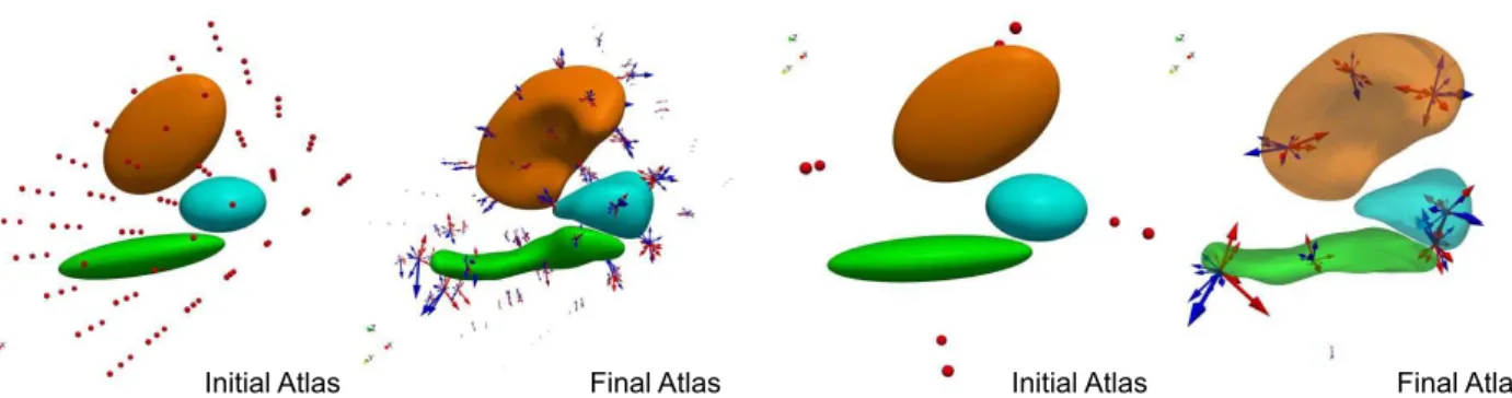
Initial Atlas Final Atlas Initial Atlas Final Atlas

a - Atlas construction with 105 control points b- Atlas construction with 8 control points

Figure 1: Atlas estimated from different initial conditions. Left: 105 control points with initial spacing equal to the deformation kernel width σV =10 mm, Right: 8 control points. Arrows are the momentum vectors of DS subjects (red) and controls (blue).

Control points that were initially on a regular lattice move to the most variable place of the shape complex during optimization. Arrows parameterize space deformations and are used as a shape descriptor of each subject in the statistical analysis.

strength to differentiate intra-group variability from inter-group differences. To discard any linear differences, including size, we co-register all shape complexes using affine transforms.

We then construct an atlas using all data, setting σV =

10 mm, σW = 5 mm, σX = σV/2 and σk = σV for all

nu-clei, and control points initially located at the nodes of regular lattice of step σV, yielding a set of 105 points. Robustness of

results with respect to these values is discussed in Sec. 3.6. The resulting template shape complex (Fig. 1-a) averages the shape characteristics of every individual in the dataset. The position of each subject’s anatomical configuration (either DS or controls) with respect to the template configuration is given by initial momentum vectors located at control point positions (arrows in Fig. 1). These momentum vectors lie in a finite-dimensional vector space, whose dimension is 3 times the num-ber of control points. Standard methods for multivariate statis-tics can be applied in this space. The resulting statisstatis-tics are expressed in terms of a set of momentum vectors. The template shape complex can be deformed in the direction pointed by the statistics via the integration of the geodesic shooting equa-tions (10) followed by the flow equaequa-tions (11). This procedure, also known as tangent-space statistics, is a way to translate the statistics into deformation patterns, and hence eases the inter-pretation of the results.

In the following sections, we show how such statistics can be computed and visualized, using the Down syndrome data as a case study.

3.1. Group differences

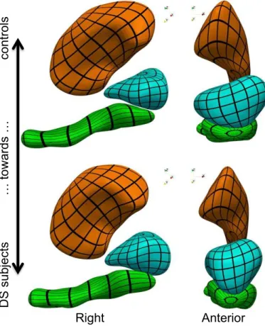
The first step is to show the differences between healthy con-trols (HC) and DS subjects that have been captured by the at-las. We compute the sample mean of the momenta for each group separately: αHC = _N1HC su P i2HC αi and αDS = _N1DS su P i2DS αi, where HC (resp. DS) denotes the set of indices corresponding to healthy controls (resp. DS subjects). We then deform the template complex in the direction of both means, thus show-ing anatomical configurations that are typical of each group (Fig. 2). The figure shows that nuclei of DS subjects are turned

toward the left part of the brain, with another torque that pushes the hippocampus tail (its posterior part) toward the superior part of the brain, and the head toward the inferior part. These two torques are more pronounced near the hippocampus/amygdala boundary than in the hippocampus tail or upper putamen re-gion. The DS subjects’ amygdala also has lesser lateral exten-sion than that of the controls.

We perform Linear Discriminant Analysis (LDA) to exhibit the most discriminative axis between both groups in the mo-menta space. For this purpose, we compute the initial veloci-ties of the control points vi _=K(c

0, c0)αi. The sample

covari-ance matrix of these velocities, assuming equal varicovari-ance in both groups, is given by:

Σ = 1 Nsu 0 B B B B B @ X i2HC (vi− vHC)⇣vi_{− v}HC⌘T+X i2DS (vi− vDS)(vi− vDS)T 1 C C C C C A. The direction of the most discriminative axis in the veloc-ity space is defined as vLDA

± = v ± Σ−1(v

HC

− vDS) where v = 1₂(vHC +vDS). The associated momentum vectors are given as: α_±LDA = K(c0, c0)−1vLDA_± . The anatomical

configu-rations are generated deforming the template shape complex in the two directions α_±LDA. We normalize the directions, so that their norm equals the norms between the means: 44

4αLDA_± 4 4 4_W⇤ = 4 4 4αHC− αDS 4 4

4_W⇤. Therefore, the sum of the geodesic distance

between the template complex and each of the deformed com-plexes is twice the norm between the means.

Results in Fig. 3 reveal similar thinning effects and torques as in Fig. 2. The figure also shows that putamen structures of DS subjects are more bent than those of controls.

Remark 3.1. Note that if the number of observations is smaller than 3 times the number of control points, then Σ is not invert-ible, and we use instead the regularized matrix Σ + "I3. In

prac-tice, we use " = 10−2, which leads to a condition number of the covariance matrix of order 1000. Statistics are not altered if this number is increased to 0.1 and 1, for which the condition number become 100 and 10 (results not shown).

Anterior

Right

Figure 2: Template complex deformed using the mean deforma-tion of controls (transparent shapes) and DS subjects (opaque shapes), which illustrates the anatomical differences that were found between both groups.

Anterior

Right

…

to

w

a

rd

s

…

co

n

tro

ls

D

S

su

b

je

ct

s

Figure 3: Most discriminative deformation axis showing the anatomical features that are the most specific to the DS subjects as compared to the controls. Differences are amplified, since the distance between the two configurations is twice the distance between the means (black grids are mapped to the surface for visualization only)

Remark 3.2. Note that we perform the statistical analysis us-ing the velocity field sampled at the control points v = K(c0, c0)α and the usual L2 inner-product. However, it would

seem more natural to use the RKHS metric on the momenta α instead. Using the RKHS metric amounts to using ˜v = K1/2_αso

that the inner-product becomes (˜vi₎T_˜vj_{= α}iT_K(c

0, c0)αj, which

is the inner-product between the velocity fields in the RKHS V. One can easily check that without regularization (" = 0), the most discriminant axis is the same in both cases, as will be the LDA and ML classification criteria introduced in the sequel. Using the identity matrix as a regularizer for the sample covari-ance matrix above amounts to using the matrix K(c0, c0)−1 as

a regularizer in the RKHS space. More precisely, the matrix Σ +"I3 becomes ˜Σ +"K(c0, c0)−1 where ˜Σis the sample

co-variance matrix of the ˜vi_{’s. It is natural to use this regularizer,}

since the criterion for atlas construction precisely assumes the momentum vectors to be distributed with a zero-mean Gaussian distribution with covariance matrix K(c0, c0)−1(which leads to

4 4 4vi0 4 4 4 2 V = α i 0 T K↵i

0 in (19)). For this reason, the same matrix

is used in Allassonni`ere et al. (2007) as a prior in a Bayesian estimation framework.

3.2. Statistical significance

We estimate the statistical significance of the above group differences using permutation tests in a multivariate setting. In our experiments, the number of subjects is always smaller than the dimension of the concatenated momentum vectors, which is 3 times the number of control points. In this case the distri-bution Hotelling T2 statistics cannot be computed and we use permutations to give an estimate of this distribution.

Let (uk, λ2_k) be the eigenvectors and eigenvalues sorted in

decreasing order of the sample covariance matrix Σ (without regularization, i.e., " = 0). We truncate the matrix up to the

Nmodeslargest eigenvalues that explain 95% of the variance: ˜Σ =

PNmodes

k=1 λ 2

kukuTk. Its inverse is given by: ˜Σ−1 =

PNmodes k=1 1 λ2 k ukuTk.

We then compute the T2_{Hotelling statistics as:}

T2 =Nsu− 2 4 (v

HC

− vDS)TΣ˜−1(vHC_{− v}DS).

To estimate the distribution of the statistics under the null hy-pothesis of equal means, we compute the statistics for 105

per-mutations of the subjects’ indices i. Each permutation changes the empirical means and within-class covariance matrices, and thus the selected subspace and the statistics. The resulting p-value equals p = 2.6 10−4, thus showing that our shape descrip-tors are significantly different between DS and HC subjects at the usual 5% level. The anatomical differences highlighted in Fig. 2 and 3 are not due to chance.

3.3. Sensitivity and specificity using cross-validation

Over-fitting is a common problem of statistical estimations in a high dimension low sample size setting. We perform leave-out experiments to evaluate the generalization errors of our model, namely its sensitivity and specificity.

We compute an atlas with the same parameter setting and initial conditions but with one control and one DS subject data

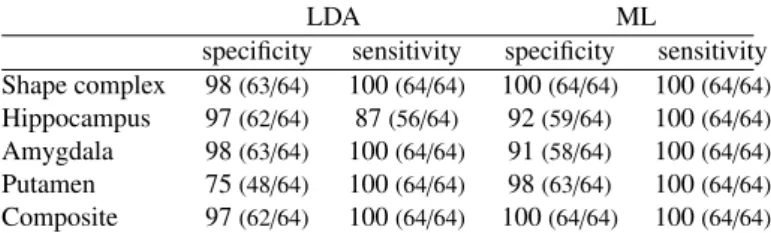
LDA ML

specificity sensitivity specificity sensitivity Shape complex 98(63/64) 100(64/64) 100(64/64) 100(64/64) Hippocampus 97(62/64) 87(56/64) 92(59/64) 100(64/64) Amygdala 98(63/64) 100(64/64) 91(58/64) 100(64/64) Putamen 75(48/64) 100(64/64) 98(63/64) 100(64/64) Composite 97(62/64) 100(64/64) 100(64/64) 100(64/64)

Table 1: Classification with 105 control points using LDA and ML classifiers. Scores (in percentage) are computed using our descriptor for shape complexes (first row), only one structure at a time (rows 2-4) or a composite descriptor (fifth row).

out, yielding 82 =64 atlases. Note that this is a design choice since one does not necessarily need to have balanced groups to apply the method. For each experiment, we register the tem-plate shape complex to each of the left-out complex by mini-mizing (19) for Nsu = 1 and considering template and control

points of the atlas fixed. The resulting momentum vectors are compared with those of the atlas. We classify them based on Maximum Likelihood (ML) ratios and LDA.

Let αtest_{be the initial momenta parameterizing the}

deforma-tion of the template shape complex to a given left-out shape complex (seen as a test data), and vtest _=K(c

0, c0)αtest. In this

section, v, vHCand vDS denotes the sample mean using only the training data (7 HC and 7 DS). In LDA, we write the classifica-tion criterion as:

C(vtest) = (vtest_{− v)}TΣ−1(vHC_{− v}DS), (22) where Σ denotes the regularized sample covariance matrix of training data (for " = 10−2, see Remark 3.1). For a threshold η, the test data is classified as healthy control if C(vtest_{) > η and}

DS subject otherwise. ROC curves are built when the thresh-old η is varied. For estimating classification scores, we esti-mate the threshold η on the training dataset so that the best separating hyperplane (orthogonal to the most discriminative axis Σ−1(vHC− vDS)) is positioned at equal distance to the two classes. This threshold value is used for classifying the test data.

For classifying in a Maximum Likelihood framework, we compute the regularized sample covariance matrices ΣDS =

1 NDs su P i_2DS (vi − vDS)(vi − vDS)T _{and Σ} HC =_N1HC su P i_2HC (vi − vHC)(vi − vHC)T_{. The classification criterion, also called the Mahalanobis}

distance, is given by:

C(vtest) = (vtest_{− v}DS)TΣ−1_DS(vtest_{− v}DS)

− (vtest− vHC)TΣ−1_HC(vtest− vHC) (23) and the classification rule remains the same.

The very high sensitivity and specificity reported in Table 1 (first row) show that the anatomical differences between DS and controls that were captured by the model are not specific to this particular dataset, but are likely to generalize well to indepen-dent datasets.

3.4. Shape complexes versus individual shapes

In this section, we aim to emphasize the differences between using a single model for the shape complex and using different models for each individual component of a shape complex.

We perform the same experiments as described above, but for each of the three structures independently. The atlas of each structure has its own set of control points and momen-tum vectors. The hypothesis of equal means for DS and con-trol subjects is rejected with a probability of false positive of

p = 3.5 10−3for the hippocampus, p = 4.7 10−3 for the puta-men and p = 1.2 10−4for the amygdala. The statistical signif-icance is lower for the hippocampus and the putamen than for the shape complex (p = 2.6 10−4), and higher for the amygdala. The classification scores reported in Table 1 (rows 2 to 4) show that none of the structures alone may predict the subject’s status with the same performance as the shape complex. Although the model for the amygdala has a higher statistical significance, it has a lower specificity in the Maximum Likelihood approach.

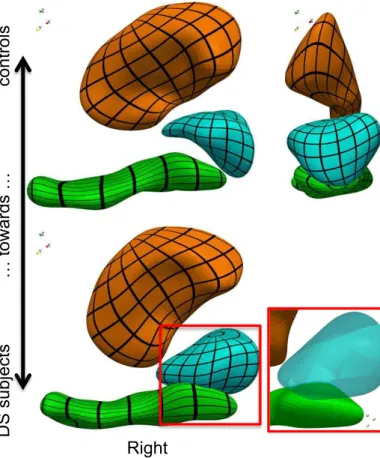
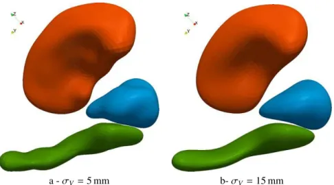
For visualization of results from individual analyses, we de-form each structure along its most discriminative axis. Be-cause the 3 deformations are not combined into a single space deformation, intersections between surfaces occur (Fig. 4). The deformation of the amygdala, though highly significant, is not compatible with the deformation of the hippocampus. From an anatomical point of view, both parts of the amyg-dala/hippocampus boundary should vary together, since almost nothing separates the two structures at the image resolution.

The shape complex analysis in Fig 2 and 3 showed that the most discriminative effects involve deformations of specific subregions, and in particular the most lower-anterior part of the complex where the amygdala is located. Therefore, it is not sur-prising that this structure shows higher statistical performance than the hippocampus and putamen in an independent analysis of each structure. However, the most discriminative deforma-tions of each structure are not consistent among themselves, thus misleading the interpretation of the findings. By contrast, the shape complex analysis shows that the discriminative effect is not specific to the amygdala but to the whole lower ante-rior part of the medial temporal lobe with strong correlations between parts of the structures within this region. The shape complex model may be slightly less significant, but it highlights shape effects that can be interpreted in the context of anatomical deformations related to underlying neurobiological processes.

One could argue that independently analyzing each ture does not take into account the correlations among struc-tures. To mimic what previously reported shape analysis meth-ods do, we build a composite shape descriptor vi _by

concate-nating the velocities of each individual atlas vi

1, v

i

2and v

i

3(for

each structure s = 1, 2, 3 and subject i, vi

s = K(c0,s, c0,s)αis

where αi

s’s are the initial momenta in each atlas). We use

this composite descriptor to compute means, sample covariance matrices, most discriminative axis and classification scores as above. This approach achieves a classification nearly as good as with the single atlas method (Table 1, last row) with a very high statistical significance p < 10−5. The direction of the most discriminative axis vLDA _{takes into account the}

Right

…

to

w

a

rd

s

…

co

n

tro

ls

D

S

su

b

je

ct

s

Figure 4: Most discriminative deformation axis computed for each structure independently. Surface intersection occurs in the absence of a global diffeomorphic constraint. (black grids are mapped to the surface for visualization only)

parameterize a single diffeomorphism– only each of its three components does. To display these correlations, we compute the initial momentum vectors associated with each component: αLDA_s = K(c0,s, c0,s)−1vLDAs for s = 1, 2, 3, and then deform

each structure using a different diffeomorphism. Even in this case, surfaces intersect, thus showing that this way of taking into account correlations does not prevent generating anatomi-cal configurations that are not compatible with the data (Inline Supplementary Figure S1). By contrast, the single atlas method proposed in this work integrates topology constraints into the analysis by the use of a single deformation of the underlying space, and therefore correctly measures correlations that pre-serve the internal organization of the anatomical complex.

3.5. Effects of dimensionality reduction

Our approach offers the possibility to control the dimen-sion of the shape descriptor by choosing the number of control points given as input to the algorithm. In 3D, the dimension of the shape descriptor is 3 times the number of control points. In this section, we evaluate the impact of this dimensionality for atlas construction and statistical estimations given our low sample size setting.

We start with 105 control points on a regular lattice with spacing equal to the deformation kernel width σV and then

Number of CP 8 12 16 24 36 105 600

Decrease of data term

(in % of initial value) 93.3 94.8 94.6 95.8 96.7 97.9 97.8

Table 2: Decrease of the data term during optimization for dif-ferent number of control points and σV =10 mm

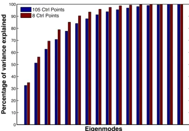
successively down-sample this lattice. With only 8 points, the number of deformation parameters is decreased by more than one order of magnitude and the initial ellipsoidal shapes still converge to a similar template shape complex (Fig. 1-b). The main reason for it is that control points are able to move to the most strategic places, noticeably at the tail of the hippocampus and the anterior part of the amygdala where the variability is the greatest. Qualitatively, the most discriminant axis is sta-ble when the dimension is varied (Inline Supplementary Fig-ure S2), as is the spectrum of the sample covariance matrices of the momentum vectors (Inline Supplementary Figure S3). The method is able to optimize the “amount” of variability captured for a given dimension of deformation parameters. Nevertheless, the residual data term at convergence increases. The initial data term (i.e., varifold norm) decreases by 97.8% for 105 points, and only by 93.3 for 8 points, thus showing that the sparsest model captured less variability in the dataset (Table 2).

If there could be an infinite number of control points, their optimal locations would be on surface meshes themselves. Therefore, one might place one control point at each ver-tex (Vaillant and Glaun`es, 2005; Ma et al., 2008). In our case, such a parameterization would involve 23058 control points. Nonetheless, this number can be arbitrarily increased or de-creased by up/down sampling of the initial ellipsoids, regardless of the variability in the dataset! We increase the number of con-trol points to 650 and notice that the estimated template shapes are the same as with 105 control points (results not shown), and that the atlas explains the same proportion of the initial data term (Table 2). Therefore, increasing the number of control points does not allow us to capture more information, which is essentially determined by the deformation kernel width σV, but

distributes this information over a larger number of parameters. This conclusion is in line with Durrleman et al. (2009), who show that such high dimensional parameterizations are very re-dundant.

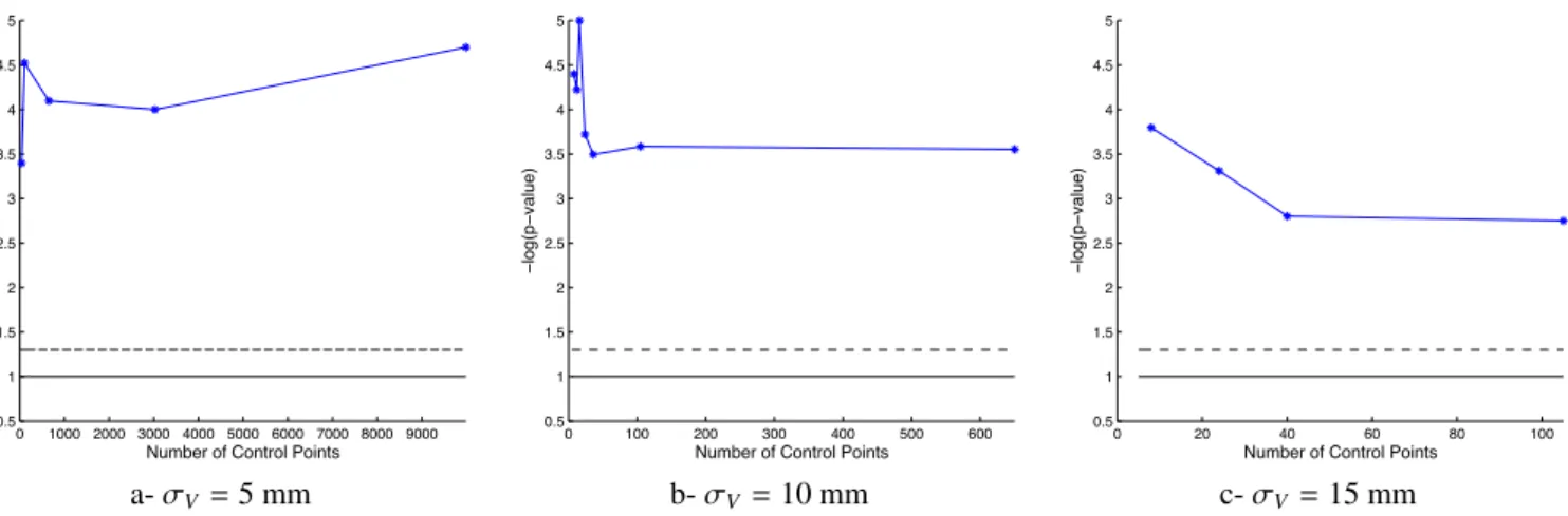
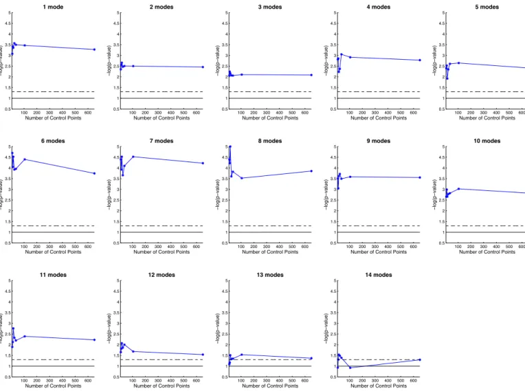
The statistical significance, as measured by the p-value as-sociated with the Hotelling T2 _{statistics, is not increased with}

higher dimensions (Fig. 5-b). It is even smaller than in small dimensions, the maximum being reached for 16 control points (p < 10−5). Leave-2-out experiments give 100% specificity and sensitivity using the ML approach, regardless of the number of control points used. To highlight differences, we performed classification using the hippocampus shape only. Again, the performance of the classifier does not necessarily decrease with the number of control points (Table 3). ROC curves in Fig. 6 show that the atlases with 48 and 18 control points have poorer performance than atlases with 12 and 8 control points.

These results suggest that using atlases of small dimension could have even greater statistical power, especially in a small sample size setting. Nevertheless, two different dimensionality

0 1000 2000 3000 4000 5000 6000 7000 8000 9000 0.5 1 1.5 2 2.5 3 3.5 4 4.5 5 − log(p − value)

Number of Control Points

0 100 200 300 400 500 600 0.5 1 1.5 2 2.5 3 3.5 4 4.5 5 − log(p − value)

Number of Control Points

0 20 40 60 80 100 0.5 1 1.5 2 2.5 3 3.5 4 4.5 5 − log(p − value)

Number of Control Points

a- σV =5 mm b- σV =10 mm c- σV =15 mm

Figure 5: Statistical significance of the group means difference for a varying number of control points. The solid (resp. dashed) lines correspond to the 0.1 (resp. 0.05) significance thresholds, respectively. The ability of the classifier to separate DS subjects to controls is little altered by the deformation kernel width σV. Increasing the number of control points, and hence the dimensionality

of the atlas, does not necessarily increase statistical performance.

reduction techniques compete with each other in these experi-ments. The first is the use of a small set of control points, which is a built-in dimensionality reduction technique, which has the advantage to optimize simultaneously the information captured in the data and the encoding of this information in a space of fixed dimension. The second is a post-hoc dimensionality re-duction using PCA when computing classification scores that project shape descriptors into the subspace, explaining 95% of the variance captured. The variation of the p-values, when the number of modes selected in the PCA is varied, shows that a number of modes optimizes the statistical significance, be-tween 6 and 8 modes (Inline Supplementary Figure S5). For each number of modes, an optimal number of control points also maximizes significance, and this number is never greater than 105 when one control point is placed at every σV.

It is difficult to distinguish the effects of the two techniques in such a low sample size setting. With 8 control points and a few dozen or more subjects, we could estimate full-rank covari-ance matrices and would not need the post-hoc dimensionality reduction techniques. A fair comparison between post-hoc and built-in dimensionality reduction would be then possible. Our hypothesis is that, in this regime, the trend of increased statisti-cal significance when the number of control points is decreased would be amplified. Indeed, the ratio between the number of variables to estimate and the number of subjects is more favor-able in such a scenario, thus making the statistical estimations more stable.

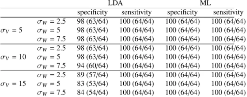
3.6. Effects of parameter settings

We assess the robustness of the results with respect to pa-rameter settings. We change the values of the deformation and varifold kernel widths by_{±50%, namely by setting σ}V =

5, 10 or 15 mm and σW=2.5, 5, or 7.5 mm. Other settings are

kept fixed, namely the weights σk =10 mm, the gradient

ker-nel width σX =0.5σV and the initial distance between control

points, which always equals σV. Classification scores are

re-ported in Table 4 and show a great robustness of the statistical

0 2.5 5 7.5 10 12.5 15 17.5 20 80 82.5 85 87.5 90 92.5 95 97.5 100

False Positive Rate (in %)

True Positive Rate (in %) _{48 Control Points}

18 Control Points 12 Control Points 8 Control Points 4 Control Points

Figure 6: ROC curves for hippocampus classification using a different number of control points in the atlas and ML classi-fier. Atlases with 48 and 18 control points exhibit poorer per-formance than those with 12 and 8 control points.

estimates, noticeably for the ML method. We note a decrease in the specificity in the LDA classifier for the large deforma-tion kernel width σV =15 mm. With large deformation kernel

widths, the atlas captures more global shape variations, which might not be as discriminative as more local changes. This ef-fect is more pronounced with increased varifold width σW, as

surface matching accuracy decreases, thus further reducing the variability captured in the atlas. These results show that the performance of the atlas is stable for a large range of reason-able values, and therefore that they are not due to fine parameter