HAL Id: hal-00797956
https://hal.archives-ouvertes.fr/hal-00797956
Submitted on 7 Mar 2013
HAL is a multi-disciplinary open access
archive for the deposit and dissemination of
sci-entific research documents, whether they are
pub-lished or not. The documents may come from
teaching and research institutions in France or
L’archive ouverte pluridisciplinaire HAL, est
destinée au dépôt et à la diffusion de documents
scientifiques de niveau recherche, publiés ou non,
émanant des établissements d’enseignement et de
recherche français ou étrangers, des laboratoires
Static and dynamic semantics of NoSQL languages
Véronique Benzaken, Giuseppe Castagna, Kim Nguyễn, Jérôme Siméon
To cite this version:
Véronique Benzaken, Giuseppe Castagna, Kim Nguyễn, Jérôme Siméon. Static and dynamic semantics
of NoSQL languages. POPL, Jan 2013, Rome, Italy. pp.101-114, �10.1145/2429069.2429083�.
�hal-00797956�
Static and Dynamic Semantics of NoSQL Languages
Véronique Benzaken
1Giuseppe Castagna
2Kim Nguy˜ên
1Jérôme Siméon
31LRI, Université Paris-Sud, Orsay, France, 2CNRS, PPS, Univ Paris Diderot, Sorbonne Paris Cité, Paris, France 3IBM Watson Research, Hawthorne, NY, USA
Abstract
We present a calculus for processing semistructured data that spans differences of application area among several novel query lan-guages, broadly categorized as “NoSQL”. This calculus lets users define their own operators, capturing a wider range of data process-ing capabilities, whilst providprocess-ing a typprocess-ing precision so far typical only of primitive hard-coded operators. The type inference algo-rithm is based on semantic type checking, resulting in type infor-mation that is both precise, and flexible enough to handle structured and semistructured data. We illustrate the use of this calculus by encoding a large fragment of Jaql, including operations and itera-tors over JSON, embedded SQL expressions, and co-grouping, and show how the encoding directly yields a typing discipline for Jaql as it is, namely without the addition of any type definition or type annotation in the code.
1.
Introduction
The emergence of Cloud computing, and the ever growing impor-tance of data in applications, has given birth to a whirlwind of new data models [19, 24] and languages. Whether they are developed under the banner of “NoSQL” [12, 35], for BigData Analytics [5, 18, 28], for Cloud computing [3], or as domain specific languages (DSL) embedded in a host language [21, 27, 32], most of them share a common subset of SQL and the ability to handle semistruc-tured data. While there is no consensus yet on the precise bound-aries of this class of languages, they all share two common traits: (i)an emphasis on sequence operations (eg, through the popular MapReduce paradigm) and (ii) a lack of types for both data and pro-grams (contrary to, say, XML programming or relational databases where data schemas are pervasive). In [21, 22], Meijer argues that such languages can greatly benefit from formal foundations, and suggests comprehensions [7, 33, 34] as a unifying model. Although we agree with Meijer for the need to provide unified, formal foun-dations to those new languages, we argue that such founfoun-dations should account for novel features critical to various application do-mains that are not captured by comprehensions. Also, most of those languages provide limited type checking, or ignore it altogether. We believe type checking is essential for many applications, with usage ranging from error detection to optimization. But we understand the designers and programmers of those languages who are averse to any kind of type definition or annotation. In this paper, we propose a calculus which is expressive enough to capture languages that go beyond SQL or comprehensions. We show how the calculus adapts to various data models while retaining a precise type checking that can exploit in a flexible way limited type information, information
An extended abstract of this work is included in the proceeding of POPL 13, 40th ACM Symposium on Principles of Programming Languages, ACM Press, 2013.
that is deduced directly from the structure of the program even in the absence of any explicit type declaration or annotation.
Example. We use Jaql [5, 18], a language over JSON [19] devel-oped for BigData analytics, to illustrate how our proposed calculus works. Our reason for using Jaql is that it encompasses all the fea-tures found in the previously cited query languages and includes a number of original ones, as well. Like Pig [28] it supports sequence iteration, filtering, and grouping operations on non-nested queries. Like AQL [3] and XQuery [6], it features nested queries. Further-more, Jaql uses a rich data model that allows arbitrary nesting of data (it works on generic sequences of JSON records whose fields can contain other sequences or records) while other languages are limited to flat data models, such as AQL whose data-model is sim-ilar to the standard relational model used by SQL databases (tuples of scalars and of lists of scalars). Lastly, Jaql includes SQL as an embedded sub-language for relational data. For these reasons, al-though in the present work we focus almost exclusively on Jaql, we believe that our work can be adapted without effort to a wide array of sequence processing languages.
The following Jaql program illustrates some of those features. It performs co-grouping [28] between one JSON input, containing information about departments, and one relational input contain-ing information about employees. The query returns for each de-partment its name and id, from the first input, and the number of high-income employees from the second input. A SQL expression is used to select the employees with income above a given value, while a Jaql filter is used to access the set of departments and the elements of these two collections are processed by the group ex-pression (in Jaql “$” denotes the current element).
group
(depts -> filter each x (x.size > 50)) by g = $.depid as ds,
(SELECT * FROM employees WHERE income > 100) by g = $.dept as es
into { dept: g,
deptName: ds[0].name, numEmps: count(es) };
The query blends Jaql expressions (eg,filterwhich selects, in the collectiondepts, departments with a sizeof more than50 employees, and the grouping itself) with a SQL statement (select-ing employees in a relational table for which the salary is more than100). Relations are naturally rendered in JSON as collections of records. In our example, one of the key difference is that field access in SQL requires the field to be present in the record, while the same operation in Jaql does not. Actually, field selection in Jaql is very expressive since it can be applied also to collections with the effect that the selection is recursively applied to the components of the collection and the collection of the results returned, and simi-larly forfilterand other iterators. In other words, the expression
filter each x (x.size > 50)above will work as much when xis bound to a record (with or without asizefield: in the latter case the selection returnsnull), as whenxis bound to a collection of records or of arbitrary nested collections thereof. This accounts for the semistructured nature of JSON compared to the relational model. Our calculus can express both, in a way that illustrates the difference in both the dynamic semantics and static typing.
In our calculus, the selection of all records whose mandatory field income is greater than 100 is defined as:
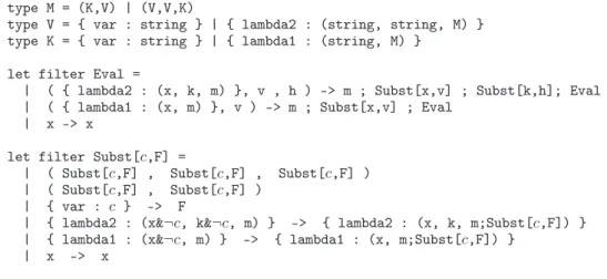
let Sel = ‘nil => ‘nil
| ({income: x, .. } as y , tail) =>
if x > 100 then (y,Sel(tail)) else Sel(tail) (collections are encoded as lists à la Lisp) while the filtering among records or arbitrary nested collections of records of those where the (optional) size field is present and larger than 50 is:
let Fil = ‘nil => ‘nil
| ({size: x, .. } as y,tail) =>
if x > 50 then (y,Fil(tail)) else Fil(tail) | ((x,xs),tail) => (Fil(x,xs),Fil(tail))
| (_,tail) => Fil(tail)
The terms above show nearly all the basic building blocks of our calculus (only composition is missing), building blocks that we dub filters. Filters can be defined recursively (eg, Sel(tail) is a recur-sive call); they can perform pattern matching as found in functional languages (the filter p ⇒⇒⇒ f executes f in the environment resulting from the matching of pattern p); they can be composed in alterna-tion (f1|||f2 tries to apply f1 and if it fails it applies f2), they can
spread over the structure of their argument (eg, (((f1,f2))) —of which
(x,Sel(tail)) is an instance— requires an argument of a prod-uct type and applies the corresponding ficomponent-wise).
For instance, the filter Fil scans collections encoded as lists à laLisp (ie, by right associative pairs with ‘nil denoting the empty list). If its argument is the empty list, then it returns the empty list; if it is a list whose head is a record with a size field (and possibly other fields matched by “. .”), then it captures the whole record in y, the content of the field in x, the tail of the list in tail, and keeps or discards y (ie, the record) according to whether x (ie, the field) is larger than 50; if the head is also a list, then it recursively applies both on the head and on the tail; if the head of the list is neither a list, nor a record with a size field, then the head is discarded. The encoding of the whole grouping query is given in Section 5.3.
Our aim is not to propose yet another “NoSQL/cloud comput-ing/bigdata analytics” query language, but rather to show how to expressand type such languages via an encoding into our core cal-culus. Each such language can in this way preserve its execution model but obtain for free a formal semantics, a type inference sys-tem and, as it happens, a prototype implementation. The type infor-mation is deduced via the encoding (without the need of any type annotation) and can be used for early error detection and debugging purposes. The encoding also yields an executable system that can be used for rapid prototyping. Both possibilities are critical in most typical usage scenarios of these languages, where deployment is very expensive both in time and in resources. As observed by Mei-jer [21] the advent of big data makes it more important than ever for programmers (and, we add, for language and system designers) to have a single abstraction that allows them to process, transform, query, analyze, and compute across data presenting utter variability both in volume and in structure, yielding a “mind-blowing number
For the sake of precision, to comply with Jaql’s semantics the last pat-tern should rather be ({..},tail) => Fil(tail): since field selection e.size fails whenever e is not a record or a list, this definition would detect the possibility of this failure by a static type error.
of new data models, query languages, and execution fabrics” [21] . The framework we present here, we claim, encompasses them all. A long-term goal is that the compilers of these languages could use the type information inferred from the encoding and the encoding itself to devise further optimizations.
Types. Pig [28], Jaql [18, 29], AQL [3] have all been conceived by considering just the map-reduce execution model. The type (or, schema) of the manipulated data did not play any role in their de-sign. As a consequence these languages are untyped and, when present, types are optional and clearly added as an afterthought. Differences in data model or type discipline are particularly im-portant when embedded in a host language (since they yield the so-called impedance mismatch). The reason why types were/are disregarded in such languages may originate in an alleged tension between type inference and heterogeneous/semistructured data: on the one hand these languages are conceived to work with collec-tions of data that are weakly or partially structured, on the other hand current languages with type inference (such as Haskell or ML) can work only on homogeneous collections (typically, lists of elements of the same type).
In this work we show that the two visions can coexist: we type data by semantic subtyping [16], a type system conceived for semi-structured data, and describe computations by our filters which are untyped combinators that, thanks to a technique of weak typing in-troduced in [9], can polymorphically type the results of data query and processing with a high degree of precision. The conception of filtersis driven by the schema of the data rather than the execution model and we use them (i) to capture and give a uniform semantics to a wide range of semi structured data processing capabilities, (ii) to give a type system that encompasses the types defined for such languages, if any, notably Pig, Jaql and AQL (but also XML query and processing languages: see Section 5.3), (iii) to infer the pre-cise result types of queries written in these languages as they are (so without the addition of any explicit type annotation/definition or new construct), and (iv) to show how minimal extensions/modifi-cations of the current syntax of these languages can bring dramatic improvements in the precision of the inferred types.
The types we propose here are extensible record types and het-erogeneous lists whose content is described by regular expressions on types as defined by the following grammar:
Types t ::= v (singleton)
| {{{ℓ:t, . . . , ℓ:t}}} (closed record) | {{{ℓ:t, . . . , ℓ:t , ...}}} (open record)
| [r] (sequences)
| int| char (base)
| any| empty | null (special)
| t|||t (union)
| t\\\t (difference)
Regexp r ::= ε | t | r* | r+ | r? | r r | r|||r where ε denotes the empty word. The semantics of types can be expressed in terms of sets of values (values are either constants —such as 1, 2, true, false, null, ’1’, the latter denoting the character 1—, records of values, or lists of values). So the single-ton type v is the type that contains just the value v (in particular null is the singleton type containing the value null). The closed record type {{{a:int, b:int}}} contains all record values with exactly two fields a and b with integer values, while the open record type {{{a:int, b:int , ...}}} contains all record values with at least two fields a and b with integer values. The sequence type [r] is the set of all sequences whose content is described by the regular expres-sionr; so, for example [char*] contains all sequences of charac-ters (we will use string to denote this type and the standard double quote notation to denote its values) while [({{{a:int}}} {{{a:int}}})+]
denotes nonempty lists of even length containing record values of type {{{a:int}}}. The union type s|||t contains all the values of s and of t, while the difference type s\\\t contains all the values of s that are not in t. We shall use bool as an abbreviation of the union of the two singleton types containing true and false: ‘true|||‘false. any and empty respectively contain all and no values. Recursive type definitions are also used (see Section 2.2 for formal details).
These types can express all the types of Pig, Jaql and AQL, all XML types, and much more. So for instance, AQL includes only homogeneous lists of type t, that can be expressed by our types as [ t* ]. In Jaql’s documentation one can find the type [ long(value=1), string(value="a"), boolean* ]which is the type of arrays whose first element is 1, the second is the string "a" and all the other are booleans. This can be easily expressed in our types as [1 "a" bool*]. But while Jaql only allows a lim-ited use of regular expressions (Kleene star can only appear in tail position) our types do not have such restrictions. So for exam-ple [char* ’@’ char* ’.’ ((’f’ ’r’)|(’i’ ’t’))] is the type of all strings (ie, sequences of chars) that denote email ad-dresses ending by either .fr or .it. We use some syntactic sugar to make terms as the previous one more readable (eg, [ .* ’@’ .* (’.fr’|’.it’)]). Likewise, henceforth we use {{{a?:t}}} to de-note that the field a of type t is optional; this is just syntactic sugar for stating that either the field is undefined or it contains a value of type t (for the formal definition see Appendix G).
Coming back to our initial example, the filter Fil defined before expects as argument a collection of the following type:
type Depts = [ ( {size?: int, ..} | Depts )* ] that is a, possibly empty, arbitrary nested list of records with an optional size field of type int: notice that it is important to specify the optional field and its type since a size field of a different type would make the expression x > 50 raise a run-time error. This information is deduced just from the structure of the filter (since Fil does not contain any type definition or annotation).
We define a type inference system that rejects any argument of Fil that has not type Depts, and deduces for arguments of type [({size: int, addr: string}| {sec: int} | Depts)+] (which is a subtype of Depts) the result type [({size: int, addr: string}|Depts)*] (so it does not forget the field addr but discards the field sec, and by replacing * for + recognizes that the test may fail).
By encoding primitive Jaql operations into a formal core cal-culus we shall provide them a formal and clean semantics as well as precise typing. So for instance it will be clear that apply-ing the followapply-ing dot selection [ [{a:3}] {a:5, b:true} ].a the result will be [ [3] 5 ] and we shall be able to deduce that _.a applied to arbitrary nested lists of records with an op-tional integer a field (ie, of type t = {{{a?:int}}} | [ t * ] ) yields arbitrary nested lists of int or null values (ie, of type u = int | null | [ u * ]).
Finally we shall show that if we accept to extend the current syntax of Jaql (or of some other language) by some minimal filter syntax (eg, the pattern filter) we can obtain a huge improvement in the precision of type inference.
Contributions. The main contribution of this work is the defini-tion of a calculus that encompasses structural operators scattered over NoSQL languages and that possesses some characteristics that make it unique in the swarm of current semi-structured data processing languages. In particular it is parametric (though fully embeddable) in a host language; it uniformly handles both width and deep nested data recursion (while most languages offer just the
The only exception are the “bags” types we did not include in order to focus on essential features.
former and limited forms of the latter); finally, it includes first-class arbitrary deep composition (while most languages offer this opera-tor only at top level), whose power is nevertheless restrained by the type system.
An important contribution of this work is that it directly com-pares a programming language approach with the tree transducer one. Our calculus implements transformations typical of top-down tree transducers but has several advantages over the transducer ap-proach: (1) the transformations are expressed in a formalism im-mediately intelligible to any functional programmer; (2) our cal-culus, in its untyped version, is Turing complete; (3) its transfor-mations can be statically typed (at the expenses of Turing com-pleteness) without any annotation yielding precise result types (4) even if we restrict the calculus only to well-typed terms (thus losing Turing completeness), it still is strictly more expressive than well-known and widely studied deterministic top-down tree transducer formalisms.
The technical contributions are (i) the proof of Turing com-pleteness for our formalism, (ii) the definition of a type system that copes with records with computable labels (iii) the definition of a static type system for filters and its correctness, (iv) the defini-tion of a static analysis that ensures the terminadefini-tion (and the proof thereof) of the type inference algorithm with complexity bounds expressed in the size of types and filters and (iv) the proof that the terms that pass the static analysis form a language strictly more expressive than top-down tree transducers.
Outline. In Section 2 we present the syntax of the three com-ponents of our system. Namely, a minimal set of expressions, the calculus of filters used to program user-defined operators or to en-code the operators of other languages, and the core types in which the types we just presented are to be encoded. Section 3 defines the operational semantics of filters and a declarative semantics for operators. The type system as well as the type inference algorithm are described in Section 4. In Section 5 we present how to han-dle a large subset of Jaql. Section 8 reports on some subtler de-sign choices of our system. We compare related works in Section 9 and conclude in Section 10. In order to avoid blurring the presen-tation, proofs, secondary results, further encodings, and extensions are moved into a separate appendix.
2.
Syntax
In this section we present the syntax of the three components of our system: a minimal set of expressions, the calculus of filters used to program user-defined operators or to encode the operators of other languages, and the core types in which the types presented in the introduction are to be encoded.
The core of our work is the definition of filters and types. The key property of our development is that filters can be grafted to any host language that satisfies minimal requirements, by simply adding filter application to the expressions of the host language. The minimal requirements of the host language for this to be possi-ble are quite simple: it must have constants (typically for types int, char, string, and bool), variables, and either pairs or record val-ues (not necessarily both). On the static side the host language must have at least basic and products types and be able to assign a type to expressions in a given type environment (ie, under some typing as-sumptions for variables). By the addition of filter applications, the host language can acquire or increase the capability to define poly-morphic user-defined iterators, query and processing expressions, and be enriched with a powerful and precise type system. 2.1 Expressions
Definition 1 (expressions).
Exprs e ::= c (constants)
| x (variables)
| (e, e) (pairs)
| {e:e, ..., e:e} (records) | e + e (record concatenation)
| e \ ℓ (field deletion)
| op(e, ..., e) (built-in operators) | f e (filter application) where f ranges over filters (defined later on), c over generic con-stants, and ℓ over string constants.
Intuitively, these expressions represent the syntax supplied by the host language —though only the first two and one of the next two are really needed— that we extend with (the missing expres-sions and) the expression of filter application. Expresexpres-sions are formed by constants, variables, pairs, records, and operation on records: record concatenation gives priority to the expression on the right. So if in r1+ r2 both records contains a field with the
same label, it is the one in r2that will be taken, while field deletion
does not require the record to contain a field with the given label (though this point is not important). The metavariable op ranges over operators as well as functions and other constructions belong-ing to or defined by the host language. Among expressions we sin-gle out a set of values, intuitively the results of computations, that are formally defined as follows:
v ::= c | (v, v) | {ℓ:v; . . . ; ℓ:v}
We use "foo" for character string constants, ’c’ for characters, 1 2 3 4 5 and so on for integers, and backquoted words, such as ‘foo, for atoms (ie, user-defined constants). We use three distin-guished atoms ‘nil, ‘true, and ‘false. Double quotes can be omitted for strings that are labels of record fields: thus we write {name:"John"} rather than {"name":"John"}. Sequences (aka, heterogeneous lists, ordered collections, arrays) are encoded à la LISP, as nested pairs where the atom ‘nil denotes the empty list. We use [e1 . . . en] as syntactic sugar for(e1, . . . , (en, ‘nil)...).
2.2 Types
Expressions, in particular filter applications, are typed by the fol-lowing set of types (typically only basic, product, recursive and —some form of— record types will be provided by the host lan-guage):
Definition 2 (types).
Types t ::= b (basic types)
| v (singleton types)
| (((t,,,t))) (products) | {{{ℓ:t, . . . , ℓ:t}}} (closed records) | {{{ℓ:t, . . . , ℓ:t , ...}}} (open records)
| t|||t (union types)
| t&&&t (intersection types) | ¬¬¬t (negation type)
| empty (empty type)
| any (any type)
| µT.t (recursive types) | T (recursion variable) | Op(t, ..., t) (foreign type calls) where every recursion is guarded, that is, every type variable is separated from its binder by at least one application of a type constructor (ie, products, records, or Op).
Most of these types were already explained in the introduction. We have basic types (int, bool, ....) ranged over by b and sin-gleton types v denoting the type that contains only the value v.
Record types come in two flavors: closed record types whose val-ues are records with exactly the fields specified by the type, and open record types whose values are records with at least the fields specified by the type. Product types are standard and we have a complete set of type connectives, that is, finite unions, intersections and negations. We use empty, to denote the type that has no values and any for the type of all values (sometimes denoted by “_” when used in patterns). We added a term for recursive types, which al-lows us to encode both the regular expression types defined in the introduction and, more generally, the recursive type definitions we used there. Finally, we use Op (capitalized to distinguish it from expression operators) to denote the host language’s type operators (if any). Thus, when filter applications return values whose type belongs just to the foreign language (eg, a list of functions) we sup-pose the typing of these functions be given by some type operators. For instance, if succ is a user defined successor function, we will suppose to be given its type in the form Arrow(int,int) and, simi-larly, for its application, say apply(succ,3) we will be given the type of this expression (presumably int). Here Arrow is a type operator and apply an expression operator.
The denotational semantics of types as sets of values, that we informally described in the introduction, is at the basis of the defi-nition of the subtyping relation for these types. We say that a type t1is a subtype of a type t2, noted t1 ≤ t2, if and only if the set
of values denoted by t1is contained (in the set-theoretic sense) in
the set of values denoted by t2. For the formal definition and the
decision procedure of this subtyping relation the reader can refer to the work on semantic subtyping [16].
2.3 Patterns
Filters are our core untyped operators. All they can do are three different things: (1) they can structurally decompose and transform the values they are applied to, or (2) they can be sequentially composed, or (3) they can do pattern matching. In order to define filters, thus, we first need to define patterns.
Definition 3 (patterns). Patterns p ::= t (type) | x (variable) | (((p,,,p))) (pair) | {{{ℓ:p, . . . , ℓ:p}}} (closed rec) | {{{ℓ:p, . . . , ℓ:p , ...}}} (open rec) | p|||p (or/union)
| p&&&p (and/intersection) where the subpatterns forming pairs, records, and intersections have distinct capture variables, and those forming unions have the same capture variables.
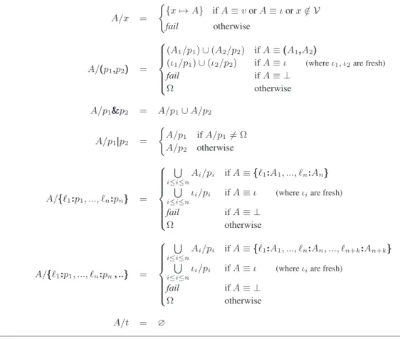
Patterns are essentially types in which capture variables (ranged over by x, y, . . . ) may occur in every position that is not under a negation or a recursion. A pattern is used to match a value. The matching of a value v against a pattern p, noted v/p, either fails (noted Ω) or it returns a substitution from the variables occurring in the pattern, into values. The substitution is then used as an environment in which some expression is evaluated. If the pattern is a type, then the matching fails if and only if the pattern is matched against a value that does not have that type, otherwise it returns the empty substitution. If it is a variable, then the matching always succeeds and returns the substitution that assigns the matched value to the variable. The pair pattern (((p1,,,p2))) succeeds if and only if it
is matched against a pair of values and each sub-pattern succeeds on the corresponding projection of the value (the union of the two substitutions is then returned). Both record patterns are similar to the product pattern with the specificity that in the open record pattern “..” matches all the fields that are not specified in the
pattern. An intersection pattern p1&&&p2 succeeds if and only if
both patterns succeed (the union of the two substitutions is then returned). The union pattern p1|||p2first tries to match the pattern p1
and if it fails it tries the pattern p2.
For instance, the pattern (((int&&&x,,,y))) succeeds only if the matched value is a pair of values (v1, v2) in which v1 is an
in-teger —in which case it returns the substitution {x/v1, y/v2}—
and fails otherwise. Finally notice that the notation “p as x” we used in the examples of the introduction, is syntactic sugar for p&&&x. This informal semantics of matching (see [16] for the formal definition) explains the reasons of the restrictions on capture vari-ables in Definition 3: in intersections, pairs, and records all patterns must be matched and, thus, they have to assign distinct variables, while in union patterns just one pattern will be matched, hence the same set of variables must be assigned, whichever alternative is se-lected.
The strength of patterns is their connections with types and the fact that the pattern matching operator can be typed exactly. This is entailed by the following theorems (both proved in [16]):
Theorem 4 (Accepted type [16]). For every patternp, the set of all valuesv such that v/p 6= Ω is a type. We call this set the accepted type of p and note it by *p+.
The fact that the exact set of values for which a matching succeeds is a type is not obvious. It states that for every pattern p there exists a syntactic type produced by the grammar in Definition 2 whose semantics is exactly the set of all and only values that are matched by p. The existence of this syntactic type, which we note *p+, is of utmost importance for a precise typing of pattern matching. In particular, given a pattern p and a type t contained in (ie, subtype of) *p+, it allows us to compute the exact type of the capture variables of p when it is matched against a value in t:
Theorem 5 (Type environment [16]). There exists an algorithm that for every patternp, and t ≤ *p+ returns a type environment t/p ∈ Vars(p) → Types such that (t/p)(x) = {(v/p)(x) | v : t}. 2.4 Filters
Definition 6 (filters). A filter is a term generated by:
Filters f ::= e (expression) | p ⇒⇒⇒ f (pattern) | (((f ,f))) (product) | {{{ℓ:f, . . . , ℓ:f , ..}}} (record) | f|||f (union) | µµµX...f (recursion) | Xa (recursive call) | f ;f (composition) | o (declarative operators) Operators o ::= groupbyf (filter grouping) | orderbyf (filter ordering)
Arguments a ::= x (variables)
| c (constants)
| (((a,a))) (pairs)
| {{{ℓ:a, ..., ℓ:a}}} (record) such that for every subterm of the form f;g, no recursion variable is free inf.
Filters are like transducers, that when applied to a value re-turn another value. However, unlike transducers they possess more “programming-oriented” constructs, like the ability to test an in-put and capture subterms, recompose an intermediary result from captured values and a composition operator. We first describe in-formally the semantics of each construct.
The expression filter e always returns the value corresponding to the evaluation of e (and discards its argument). The filter p ⇒⇒⇒ f applies the filter f to its argument in the environment obtained by matching the argument against p (provided that the matching does not fail). This rather powerful feature allows a filter to perform two critical actions: (i) inspect an input with regular pattern-matching before exploring it and (ii) capture part of the input that can be reused during the evaluation of the subfilter f. If the argument ap-plication of fito vireturns v′ithen the application of the product
filter (((f1,f2))) to an argument (v1, v2) returns (v1′, v2′); otherwise, if
any application fails or if the argument is not a pair, it fails. The record filter is similar: it applies to each specified field the corre-sponding filter and, as stressed by the “. .”, leaves the other fields unchanged; it fails if any of the applications does, or if any of the specified fields is absent, or if the argument is not a record. The fil-ter f1|||f2returns the application of f1to its argument or, if this fails,
the application of f2. The semantics of a recursive filter is given by
standard unfolding of its definition in recursive calls. The only real restriction that we introduce for filters is that recursive calls can be done only on arguments of a given form (ie, on arguments that have the form of values where variables may occur). This restriction in practice amounts to forbid recursive calls on the result of another recursively defined filter (all other cases can be easily encoded). The reason of this restriction is technical, since it greatly simpli-fies the analysis of Section 4.5 (which ensures the termination of type inference) without hampering expressiveness: filters are Tur-ing complete even with this restriction (see Theorem 7). Filters can be composed: the filter f1;f2 applies f2 to the result of applying
f1to the argument and fails if any of the two does. The condition
that in every subterm of the form f;g, f does not contain free re-cursion variables is not strictly necessary. Indeed, we could allow such terms. The point is that the analysis for the termination of the typing would then reject all such terms (apart from trivial ones in which the result of the recursive call is not used in the composition). But since this restriction does not restrict the expressiveness of the calculus (Theorem 7 proves Turing completeness with this restric-tion), then the addition of this restriction is just a design (rather than a technical) choice: we prefer to forbid the programmer to write recursive calls on the left-hand side of a composition, than systematically reject all the programs that use them in a non-trivial way.
Finally, we singled out some specific filters (specifically, we chose groupby and orderby ) whose semantics is generally specified in a declarative rather than operational way. These do not bring any expressive power to the calculus (the proof of Turing completeness, Theorem 7, does not use these declarative operators) and actually they can be encoded by the remaining filters, but it is interesting to single them out because they yield either simpler encodings or more precise typing.
3.
Semantics
The operational semantics of our calculus is given by the reduction semantics for filter application and for the record operations. Since the former is the only novelty of our work, we save space and omit the latter, which are standard anyhow.
3.1 Big step semantics
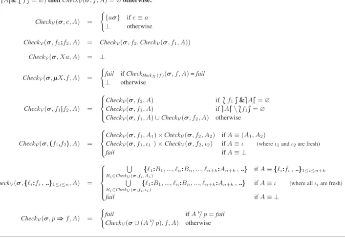
We define a big step operational semantics for filters. The definition is given by the inference rules in Figure 1 for judgements of the form δ;γ ⊢eval f (a) r and describes how the evaluation of
the application of filter f to an argument a in an environment γ yields an object r where r is either a value or Ω. The latter is a special value which represents a runtime error: it is raised by the rule (error) either because a filter did not match the form of its argument (eg, the argument of a filter product was not a pair)
(expr)
δ;γ ⊢evale(v) r r = eval(γ, e)
(prod) δ;γ ⊢evalf1(v1) r1 δ;γ ⊢evalf2(v2) r2
δ;γ ⊢eval(((f1,f2)))(v1, v2) (r1, r2)
if r16= Ω
and r26= Ω
(patt) δ;γ , v/p ⊢evalf (v) r
δ;γ ⊢eval(p ⇒⇒⇒ f )(v) r if v/p 6= Ω
(comp) δ;γ ⊢evalf1(v) r1 δ;γ ⊢evalf2(r1) r2
δ;γ ⊢eval(f1;f2)(v) r2 if r16= Ω
(union1) δ;γ ⊢evalf1(v) r1
δ;γ ⊢eval(f1|||f2)(v) r1 if r16= Ω
(union2) δ;γ ⊢evalf1(v) Ω δ;γ ⊢evalf2(v) r2
δ;γ ⊢eval(f1|||f2)(v) r2
(rec) δ, (X 7→ f );γ ⊢evalf (v) r
δ;γ ⊢eval(µµµX...f )(v) r
(rec-call) δ;γ ⊢eval(δ(X))(a) r
δ;γ ⊢eval(Xa)(v) r
(error)
δ;γ ⊢evalf (a) Ω if no other rule applies
(recd) δ;γ ⊢evalf1(v1) r1 · · · δ;γ ⊢evalfn(vn) rn
δ;γ ⊢eval{{{ℓ1:f1, ..., ℓn:fn, ..}}}({{{ℓ1:v1, ..., ℓn:vn, ..., ℓn+k:vn+k}}}) {{{ℓ1:r1, ..., ℓn:rn, ..., ℓn+k:vn+k}}} if ∀i, ri6= Ω
Figure 1. Dynamic semantics of filters or because some pattern matching failed (ie, the side condition
of (patt) did not hold). Notice that the argument a of a filter is always a value v unless the filter is the unfolding of a recursive call, in which case variables may occurr in it (cf. rule rec-call). Environment δ is used to store the body of recursive definitions.
The semantics of filters is quite straightforward and inspired by the semantics of patterns. The expression filter discards its input and evaluates (rather, asks the host language to evaluate) the expression e in the current environment (expr). It can be thought of as the right-hand side of a branch in a match_with construct.
The product filter expects a pair as input, applies its sub-filters component-wise and returns the pair of the results (prod). This filter is used in particular to express sequence mapping, as the first component f1 transforms the element of the list and f2is applied
to the tail. In practice it is often the case that f2is a recursive call
that iterates on arbitrary lists and stops when the input is ‘nil. If the input is not a pair, then the filter fails (rule (error) applies).
The record filter expects as input a record value with at least the same fields as those specified by the filter. It applies each sub-filter to the value in the corresponding field leaving the contents of other fields unchanged (recd). If the argument is not a record value or it does not contain all the fields specified by the record filter, or if the application of any subfilter fails, then the whole application of the record filter fails.
The pattern filter matches its input value v against the pattern p. If the matching fails so the filter does, otherwise it evaluates its sub-filter in the environment augmented by the substitution v/p (patt). The alternative filter follows a standard first-match policy: If the filter f1succeeds, then its result is returned (union-1). If f1fails,
then f2is evaluated against the input value (union-2). This filter is
particularly useful to write the alternative of two (or more) pattern filters, making it possible to conditionally continue a computation based on the shape of the input.
The composition allows us to pass the result of f1as input to f2.
The composition filter is of paramount importance. Indeed, without it, our only way to iterate (deconstruct) an input value is to use a productfilter, which always rebuilds a pair as result.
Finally, a recursive filter is evaluated by recording its body in δ and evaluating it (rec), while for a recursive call we replace the recursion variable by its definition (rec-call).
This concludes the presentation of the semantics of non-declarative filters (ie, without groupby and orderby). These form a Turing complete formalism (full proof in Appendix B):
Theorem 7 (Turing completeness). The language formed by constants, variables, pairs, equality, and applications of non-declarative filters is Turing complete.
Proof(sketch). We can encode untyped call-by-value λ-calculus by first applying continuation passing style (CPS) transformations and encoding CPS term reduction rules and substitutions via filters. Thanks to CPS we eschew the restrictions on composition. 3.2 Semantics of declarative filters
To conclude the presentation of the semantics we have to define the semantics of groupby and orderby. We prefer to give the semantics in a declarative form rather than operationally in order not to tie it to a particular order (of keys or of the execution):
Groupby: groupbyf applied to a sequence [v1. . . vm] reduces
to a sequence [ (k1, l1) . . . (kn, ln) ] such that:
1. ∀i, 1 ≤ i ≤ m, ∃j, 1 ≤ j ≤ n, s.t. kj= f (vi) 2. ∀j, 1 ≤ j ≤ n, ∃i, 1 ≤ i ≤ m, s.t. kj= f (vi) 3. ∀j, 1 ≤ j ≤ n, ljis a sequence: [ vj1. . . vnjj] 4. ∀j, 1 ≤ j ≤ n, ∀k, 1 ≤ k ≤ nj, f(vkj) = kj 5. ki= kj⇒ i = j 6. l1, . . . , lnis a partition of [v1. . . vm]
Orderby: orderbyf applied to [v1. . . vn] reduces to [v1′. . . v′n]
such that: 1. [v′
1. . . vn′] is a permutation of [v1. . . vn],
2. ∀i, j s.t. 1 ≤ i ≤ j ≤ n, f(vi) ≤ f (vj)
Since the semantics of both operators is deeply connected to a notion of equality and order on values of the host language, we give them as “built-in” operations. However we will illustrate how our type algebra allows us to provide very precise typing rules, specialized for their particular semantics. It is also possible to encode co-grouping (or groupby on several input sequences) with a combination of groupby and filters (cf. Appendix H).
3.3 Syntactic sugar
Now that we have formally defined the semantics of filters we can use them to introduce some syntactic sugar.
Expressions. The reader may have noticed that the productions for expressions (Definition 1) do not define any destructor (eg, projections, label selection, . . . ), just constructors. The reason is that destructors, as well as other common expressions, can be encoded by filter applications:
e.ℓ = ({{{ℓ:x , ..def ....}}} ⇒⇒⇒ x)e fst(e) = ((((x,,,any))) ⇒def ⇒⇒ x)e snd(e) = ((((any,,,x))) ⇒def ⇒⇒ x)e letp = e1ine2
def
= (p ⇒⇒⇒ e2)e1
matche with p1⇒⇒⇒ e1|...|pn⇒⇒⇒ en
def
= (p1⇒⇒⇒ e1||| . . . |||pn⇒⇒⇒ en)e
These are just a possible choice, but others are possible. For in-stance in Jaql dot selection is overloaded: when _.ℓ is applied to a record, Jaql returns the content of its ℓ field; if the field is ab-sent or the argument is null, then Jaql returns null and fails if the argument is not a record; when applied to a list (‘array’ in Jaql terminology) it recursively applies to all the elements of the list. So Jaql’s “_.ℓ” is precisely defined as
µµµX...({{{ℓ:x , ...}}} ⇒⇒⇒ x ||| ({{{..}}}|||null) ⇒⇒⇒ null ||| (((h,,,t))) ⇒⇒⇒ (((Xh,Xt )))) Besides the syntactic sugar above, in the next section we will use t1+ t2 to denote the record type formed by all field types in t2
and all the field types in t1whose label is not already present in t2.
Similarly t \ ℓ will denote the record types formed by all field types in t apart from the one labelled by ℓ, if present. Finally, we will also use for expressions, types, and patterns the syntactic sugar for lists used in the introduction. So, for instance, [p1p2... pn] is matched
by lists of n elements provided that their i-th element matches pi.
4.
Type inference
In this section we describe a type inference algorithm for our expressions.
4.1 Typing of simple and foreign expressions
Variables, constants, and pairs are straightforwardly typed by
[VARS] Γ ⊢ x : Γ(x) [CONSTANT] Γ ⊢ c : c [PROD] Γ ⊢ e1: t1 Γ ⊢ e2: t2 Γ ⊢ (e1, e2) : (((t1,,,t2)))
where Γ denotes a typing environment that is a function from ex-pression variables to types and c denotes both a constant and the singleton type containing the constant. Expressions of the host lan-guage are typed by the type function which given a type environ-ment and a foreign expression returns the type of the expression, and that we suppose to be given for each host language.
[FOREIGN]
Γ ⊢ e1: t1 · · · Γ ⊢ en: tn
Γ ⊢ op(e1,..., en) : type((Γ, x1:t1, ..., xn:tn), op(x1,..., xn))
Since the various eican contain filter applications, thus unknown
to the host language’s type system, the rule [FOREIGN] swaps them with variables having the same type.
Notice that our expressions, whereas they include filter appli-cations, do not include applications of expressions to expressions. Therefore if the host language provides function definitions, then the applications of the host language must be dealt as foreign ex-pressions, as well (cf. the expression operator apply in Section 2.2). 4.2 Typing of records
The typing of records is novel and challenging because record ex-pressions may contain string exex-pressions in label position, such as in {{{e1:e2}}}, while in all type systems for record we are aware of,
labels are never computed. It is difficult to give a type to {{{e1:e2}}}
since, in general, we do not statically know the value that e1 will
return, and which is required to form a record type. All we can (and must) ask is that this value will be a string. To type a record expression {{{e1:e2}}}, thus, we distinguish two cases according to
The function type must be able to handle type environments with types of our system. It can do it either by subsuming variable with specific types to the types of the host language (eg, if the host language does not support singleton types then the singleton type 3 will be subsumed to int) or by typing foreign expressions by using our types.
whether the type t1of e1is finite (ie, it contains only finitely many
values, such as, say, Bool) or not. If a type is finite, (finiteness of regular types seen as tree automata can be decided in polynomial time [10]), then it is possible to write it as a finite union of values (actually, of singleton types). So consider again {{{e1:e2}}} and let t1
be the type of e1 and t2 the type of e2. First, t1 must be a
sub-type of string (since record labels are strings). So if t1 is finite
it can be expressed as ℓ1||| · · · |||ℓnwhich means that e1 will return
the string ℓifor some i ∈ [1..n]. Therefore {{{e1:e2}}} will have type
{{{ℓi: t2}}} for some i ∈ [1..n] and, thus, the union of all these types,
as expressed by the rule [RCD-FIN] below. If t1is infinite instead,
then all we can say is that it will be a record with some (unknown) labels, as expressed by rule [RCD-INF].
[RCD-FIN] Γ ⊢ e : ℓ1||| · · · |||ℓn Γ ⊢ e′: t Γ ⊢ {e:e′} : {{{ℓ 1:t}}}||| · · · |||{{{ℓn:t}}} [RCD-INF] Γ ⊢ e : t Γ ⊢ e′: t′ t ≤ string t is infinite Γ ⊢ {e:e′} : {{{..}}} [RCD-MUL] Γ ⊢ {e1:e′1} : t1 · · · Γ ⊢ {en:e′n} : tn Γ ⊢ {e1:e′1, . . . , en:e′n} : t1+ · · · + tn [RCD-CONC] Γ ⊢ e1: t1 Γ ⊢ e2: t2 t1≤ {{{..}}} t2≤ {{{..}}} Γ ⊢ e1+ e2: t1+ t2 [RCD-DEL] Γ ⊢ e : t t ≤ {{{..}}} Γ ⊢ e \ ℓ : t \ ℓ
Records with multiple fields are handled by the rule [RCD-MUL]
which “merges” the result of typing single fields by using the type operator + as defined in CDuce [4, 15], which is a right-priority record concatenation defined to take into account undefined and unknown fields: for instance, {{{a:int, b:int}}} + {{{a?:bool}}} = {{{a:int|||bool, b:int}}}; unknown fields in the right-hand side may override known fields of the left-hand side, which is why, for in-stance, we have {{{a:int, b:bool}}} + {{{b:int , ...}}} = {{{b:int , ...}}}; likewise, for every record type t (ie, for every t subtype of {{{..}}}) we have t + {{{..}}} = {{{..}}}.Finally, [RCD-CONC] and [RCD-DEL] deal with record concatenation and field deletion, respectively, in a straightforward way: the only constraint is that all expressions must have a record type (ie, the constraints of the form ... ≤ {{{..}}}). See Appendix G for formal definitions of all these type operators.
Notice that these rules do not ensure that a record will not have two fields with the same label, which is a run-time error. Detect-ing such an error needs sophisticated type systems (eg, dependent types) beyond the scope of this work. This is why in the rule [RCD -MUL] we used type operator “+” which, in case of multiple occur-ring labels, since records are unordered, corresponds to randomly choosing one of the types bound to these labels: if such a field is selected, it would yield a run-time error, so its typing can be am-biguous. We can fine tune the rule [RCD-MUL] so that when all the
tiare finite unions of record types, then we require to have pairwise
disjoint sets of labels; but since the problem would still persist for infinite types we prefer to retain the current, simpler formulation. 4.3 Typing of filter application
Filters are not first-class: they can be applied but not passed around or computed. Therefore we do not assign types to filters but, as for any other expression, we assign types to filter applications. The typing rule for filter application
[FILTER-APP]
Γ ⊢ e : t Γ ;∅ ;∅ ⊢filf (t) : s
relies on an auxiliary deduction system for judgments of the form Γ ;∆ ;M ⊢fil f (t) : s that states that if in the environments
Γ, ∆, M (explained later on) we apply the filter f to a value of type t, then it will return a result of type s.
To define this auxiliary deduction system, which is the core of our type analysis, we first need to define *f+, the type accepted by a filter f. Intuitively, this type gives a necessary condition on the input for the filter not to fail:
Definition 8 (Accepted type). Given a filter f, the accepted type of f, written *f+ is the set of values defined by:
*e+ = any
*p ⇒⇒⇒ f + = *p + &&& * f + *f1|||f2+ = *f1+ ||| * f2+ *(((f1,f2)))+ = ((( * f1+ ,,, * f2+ ))) *f1;f2+ = *f1+ *Xa+ = any *µµµX...f + = *f + *groupby f + = [any*] *orderby f + = [any*] *{{{ℓ1:f1,.., ℓn:fn, ..}}}+ = {{{ℓ1:* f1+ ,.., ℓn:* f2+ , ...}}}
It is easy to show that an argument included in the accepted type is a necessary (but not sufficient, because of the cases for composition and recursion) condition for the evaluation of a filter not to fail: Lemma 9. Letf be a filter and v be a value such that v /∈ *f +. For everyγ, δ, if δ;γ ⊢evalf (v) r, then r ≡ Ω.
The proof is a straightforward induction on the structure of the derivation, and is detailed in Appendix C. The last two auxiliary definitions we need are related to product and record types. In the presence of unions, the most general form for a product type is a finite union of products (since intersections distribute on products). For instance consider the type
(((int,,,int)))|||(((string,,,string)))
This type denotes the set of pairs for which either both projections are int or both projections are string. A type such as
(((int|||string,,,int|||string)))
is less precise, since it also allows pairs whose first projection is an int and second projection is a string and vice versa. We see that it is necessary to manipulate finite unions of products (and similarly for records), and therefore, we introduce the following notations: Lemma 10 (Product decomposition). Lett ∈ Types such that t ≤ (((any,,,any))). A product decomposition of t, denoted by πππ(t) is a set of types: π π π(t) = {(((t1 1,,,t12))), . . . , (((tn1,,,tn2)))} such thatt = W
ti∈πππ(t)ti. For a given product decomposition, we
say thatn is the rank of t, noted rank(t), and use the notation πππj
i(t) for the type t j i.
There exist several suitable decompositions whose details are out of the scope of this paper. We refer the interested reader to [15] and [23] for practical algorithms that compute such decompositions for any subtype of (((any,,,any))) or of {{{...}}}. These notions of decom-position, rank and projection can be generalized to records: Lemma 11 (Record decomposition). Lett ∈ Types such that t ≤ {{{..}}}. A record decomposition of t, denoted by ρρρ(t) is a finite set of typesρρρ(t)={r1, . . . , rn} where each riis either of the form
{{{ℓi 1:ti1, . . . , ℓini:t i ni}}} or of the form {{{ℓ i 1:ti1, . . . , ℓini:t i ni,...}}} and such thatt = W
ri∈ρρρ(t)ri. For a given record decomposition, we
say thatn is the rank of t, noted rank(t), and use the notation ρρρjℓ(t)
for the type of labelℓ in the jth
component ofρρρ(t).
In our calculus we have three different sets of variables. The set Vars of term variables, ranged over by x, y, ..., introduced in patterns and used in expressions and in arguments of calls of recursive filters. The set RVars of term recursion variables, ranged over by X, Y, ... and that are used to define recursive filters. The set TVars of type recursion variables, ranged over by T, U, ... used
to define recursive types. In order to use them we need to define three different environments: Γ : Vars → Types denoting type environmentsthat associate term variables with their types; ∆ : RVars → Filters denoting definition environments that associate each filter recursion variable with the body of its definition; M : RVars× Types → TVars denoting memoization environments which record that the call of a given recursive filter on a given type yielded the introduction of a fresh recursion type variable. Our typing rules, thus work on judgments of the form Γ ;∆ ;M ⊢ f (t) : t′stating that applying f to an expression of type t in the environments Γ, ∆, M yields a result of type t′. This judgment
can be derived with the set of rules given in Figure 2.
These rules are straightforward, when put side by side with the dynamic semantics of filters, given in Section 3. It is clear that this type system simulates at the level of types the computations that are carried out by filters on values at runtime. For instance, rule[FIL -EXPR]calls the typing function of the host language to determine the type of an expression e. Rule[FIL-PROD]applies a product filter recursively on the first and second projection for each member of the product decomposition of the input type and returns the union of all result types. Rule[FIL-REC]for records is similar, recursively applying sub-filters label-wise for each member of the record de-composition and returning the union of the resulting record types. As for the pattern filter (rule[FIL-PAT]), its subfilter f is typed in the environment augmented by the mapping t/p of the input type against the pattern (cf. Theorem 5). The typing rule for the union filter,[FIL-UNION]reflects the first match policy: when typing the second branch, we know that the first was not taken, hence that at runtime the filtered value will have a type that is in t but not in *f1+.
Notice that this is not ensured by the definition of accepted type — which is a rough approximation that discards grosser errors but, as we stressed right after its definition, is not sufficient to ensure that evaluation of f1will not fail— but by the type system itself:
the premises check that f1(t1) is well-typed which, by induction,
implies that f1 will never fail on values of type t1 and, ergo, that
these values will never reach f2. Also, we discard from the output type the contribution of the branches that cannot be taken, that is, branches whose accepted type have an empty intersection with the input type t. Composition (rule[FIL-COMP]) is straightforward. In this rule, the restriction that f1 is a filter with no open recursion
variable ensures that its output type s is also a type without free recursion variables and, therefore, that we can use it as input type for f2. The next three rules work together. The first,[FIL-FIX] intro-duces for a recursive filter a fresh recursion variable for its output type. It also memoize in ∆ that the recursive filter X is associated with a body f and in M that for an input filter X and an input type t, the output type is the newly introduced recursive type variable. When dealing with a recursive call X two situations may arise. One possibility is that it is the first time the filter X is applied to the input type t. We therefore introduce a fresh type variable T and recurse, replacing X by its definition f. Otherwise, if the input type has already been encountered while typing the filter variable X, we can return its memoized type, a type variable T . Finally, Rule[FIL-ORDBY]and Rule[FIL-GRPBY]handle the special cases of groupby and orderby filters. Their typing is explained in the following section.
4.4 Typing oforderby and groupby
While the “structural” filters enjoy simple, compositional typing rules, the ad-hoc operations orderby and groupby need specially crafted rules. Indeed it is well known that when transformation languages have the ability to compare data values type-checking (and also type inference) becomes undecidable (eg, see [1, 2]). We therefore provide two typing approximations that yield a good
[FIL-EXPR]
Γ ;∆ ;M ⊢file(t) : type(Γ, e,)
[FIL-PAT]
Γ ∪ t/p ;∆ ;M ⊢filf (t) : s
t≤ *p + &&& * f +
Γ ;∆ ;M ⊢filp ⇒⇒⇒ f (t) : s [FIL-PROD] i=1..rank(t), j=1, 2 Γ ;∆ ;M ⊢filfj(πππij(t)) : sij Γ ;∆ ;M ⊢fil(((f1,f2)))(t) : _ i=1..rank(t) (((si 1,,,si2))) [FIL-REC] i=1..rank(t), j=1..m Γ ;∆ ;M ⊢filfj(ρρρiℓj(t)) : s i j Γ ;∆ ;M ⊢fil{{{ℓ1:f1, . . . , ℓm:fm, ..}}}(t) : _ i=1..rank(t) { {{ℓ1:si1, . . . , ℓm:sim,...}}} [FIL-UNION] i = 1, 2 Γ ;∆ ;M ⊢filfi(ti) : si t≤ *f1+ ||| * f2+
t1= t&&& * f1+ t2= t&&&¬*f1+
Γ ;∆ ;M ⊢filf1|||f2(t) : _ {i|si6=empty} si [FIL-COMP] Γ ;∆ ;M ⊢filf1(t) : s Γ ;∆ ;M ⊢filf2(s) : s′ Γ ;∆ ;M ⊢filf1;f2(t) : s′ [FIL-FIX] Γ ;∆, (X 7→ f ) ;M, ((X, t) 7→ T ) ⊢filf (t) : s Tfresh Γ ;∆ ;M ⊢fil(µµµX...f )(t) : µµµT ...s [FIL-CALL-NEW] Γ ;∆ ;M, ((X, t) 7→ T ) ⊢fil∆(X)(t) : t′ t= type(Γ, a) (X, t) 6∈ dom(M) Tfresh Γ ;∆ ;M ⊢fil(Xa)(s) : µµµT ...t′ [FIL-CALL-MEM] t= type(Γ, a) (X, t) ∈ dom(M) Γ ;∆ ;M ⊢fil(Xa)(s) : M (X, t) [FIL-ORDBY]
∀ti∈ item(t) Γ ;∆ ;M ⊢filf (ti) : si tW≤ [any*] isiis ordered
Γ ;∆ ;M ⊢fil(orderby f )(t) : OrderBy(t)
[FIL-GRPBY]
∀ti∈ item(t) Γ ;∆ ;M ⊢filf (ti) : si
t≤ [any*]
Γ ;∆ ;M ⊢fil(groupby f )(t) : [((((Wisi),OrderBy(t))))*]
Figure 2. Type inference algorithm for filter application compromise between precision and decidability. First we define an
auxiliary function over sequence types:
Definition 12 (Item set). Let t ∈ Types such that t ≤ [any*]. The item set of t denoted by item(t) is defined by:
item(empty) = ∅
item(t) = item(t&&&(((any,any)))) if t 6≤ (((any,any))) item(_ 1≤i≤rank(t) (((t1i,,,t2i)))) = [ 1≤i≤rank(t) ({t1i} ∪ item(t2i))
The first and second line in the definition ensure that item() returns the empty set for sequence types that are not products, namely for the empty sequence. The third line handles the case of non-empty sequence type. In this case t is a finite union of products, whose first components are the types of the “head” of the sequence and second components are recursively the types of the tails. Note also that this definition is well-founded. Since types are regular trees the number of distinct types accumulated by item() is finite. We can now defined typing rules for the orderby and groupby operators. orderby f : The orderby filter uses its argument filter f to compute a key from each element of the input sequence and then returns the same sequence of elements, sorted with respect to their key. Therefore, while the types of the elements in the result are still known, their order is lost. We use item() to compute the output type of an orderby application:
OrderBy(t) = [(_
ti∈item(t)
ti) ∗ ]
groupbyf : The typing of orderby can be used to give a rough approximation of the typing of groupby as stated by rule [FIL -GRPBY]. In words, we obtain a list of pairs where the key com-ponent is the result type of f applied to the items of the sequence, and use OrderBy to shuffle the order of the list. A far more pre-cise typing of groupby that keeps track of the relation between list elements and their images via f is given in Appendix E.
4.5 Soundness, termination, and complexity
The soundness of the type inference system is given by the property of subject reduction for filter application
Theorem 13 (subject reduction). If∅ ;∅ ;∅ ⊢fil f (t) : s, then
for allv : t, ∅;∅ ⊢evalf (v) r implies r : s.
whose full proof is given in Appendix C. It is easy to write a fil-ter for which the type inference algorithm, that is the deduction of ⊢fil, does not terminate: µµµX...x ⇒⇒⇒ X(((x,x))). The deduction of
Γ ;∆ ;M ⊢fil f (t) : s simulates an (abstract) execution of the
filter f on the type t. Since filters are Turing complete, then in general it is not possible to decide whether the deduction of ⊢fil
for a given filter f will terminate for every input type t. For this reason we define a static analysis Check(f) for filters that ensures that if f passes the analysis, then for every input type t the deduc-tion of Γ ;∆ ;M ⊢fil f (t) : s terminates. For space reasons the
formal definition of Check(f) is relegated to Appendix A, but its behavior can be easily explained. Imagine that a recursive filter f is applied to some input type t. The algorithm tracks all the recur-sive calls occurring in f; next it performs one step of reduction of each recursive call by unfolding the body; finally it checks in this unfolding that if a variable occurs in the argument of a recursive call, then it is bound to a type that is a subtree of the original type t. In other words, the analysis verifies that in the execution of the derivation for f(t) every call to s/p for some type s and pattern p always yields a type environment where variables used in re-cursive calls are bound to subtrees of t. This implies that the rule
[FIL-CALL-NEW]will always memoize for a given X, types that are obtained from the arguments of the recursive calls of X by replac-ing their variables with a subtree of the original type t memoized by the rule[FIL-FIX]. Since t is regular, then it has finitely many distinct subtrees, thus[FIL-CALL-NEW]can memoize only finitely many distinct types, and therefore the algorithm terminates.
More precisely, the analysis proceeds in two passes. In the first pass the algorithm tracks all recursive filters and for each of them it (i) marks the variables that occur in the arguments of its recursive calls, (ii) assigns to each variable an abstract identifier represent-ing the subtree of the input type to which the variable will be bound at the initial call of the filter, and (iii) it returns the set of all types obtained by replacing variables by the associated abstract identifier in each argument of a recursive call. The last set intuitively repre-sents all the possible ways in which recursive calls can shuffle and recompose the subtrees forming the initial input type. The second phase of the analysis first abstractly reduces by one step each re-cursive filter by applying it on the set of types collected in the first phase of the analysis and then checks whether, after this reduction, all the variables marked in the first phase (ie, those that occur in ar-guments of recursive calls) are still bound to subtrees of the initial input type: if this checks fails, then the filter is rejected.
It is not difficult to see that the type inference algorithm con-verges if and only if for every input type there exists a integer n such that after n recursive calls the marked variables are bound only to subtrees of the initial input type (or to something that does not depend on it, of course). Since deciding whether such an n exists is not possible, our analysis checks whether for all possible input types a filter satisfies it for n=1, that is to say, that at every recursive call its marked variables satisfy the property; otherwise it rejects the filter.
Theorem 14 (Termination). If Check(f ), then for every type t the deduction ofΓ ;∅ ;∅ ⊢filf (t) : s is in 2-EXPTIME. Furthermore,
ift is given as a non-deterministic tree automaton (NTA) then Γ ;∅ ;∅ ⊢filf (t) : s is in EXPTIME, where the size of the problem
is|f | × |t|.
(for proofs see Appendix A for termination and Appendix D for complexity). This complexity result is in line with those of similar formalisms. For instance in [20], it is shown that type-checking non deterministic top-down tree transducers is in EXPTIME when the input and output types are given by a NTA.
All filters defined in this paper (excepted those in Appendix B) pass the analysis. As an example consider the filter rotate that ap-plied to a list returns the same list with the first element moved to the last position (and the empty list if applied to the empty list):
µ
µµX... ( (((x,(((y,z)))))) ⇒⇒⇒ (((y,X(((x,z)))))) ||| w ⇒⇒⇒ w )
The analysis succeeds on this filter. If we denote by ιxthe abstract
subtree bound to the variable x, then the recursive call will be ex-ecuted on the abstract argument (((ιx,ιz))). So in the unfolding of the
recursive call x is bound to ιx, whereas y and z are bound to two
distinct subtrees of ιz. The variables in the recursive call, x and z,
are thus bound to subtrees of the original tree (even though the ar-gument of the recursive call is not a subtree of the original tree), therefore the filter is accepted . In order to appreciate the precision of the inference algorithm consider the type [int+ bool+], that is, the type of lists formed by some integers (at least one) followed by some booleans (at least one). For the application of rotate to an argument of this type our algorithm statically infers the most pre-cise type, that is, [int* bool+ int]. If we apply it once more the inferred type is [int* bool+ int int]|[bool* int bool]. Generic filters are Turing complete. However, requiring that Check() holds —meaning that the filter is typeable by our system— restricts the expressive power of our filters by preventing them from recomposing a new value before doing a recursive call. For instance, it is not possible to typecheck a filter which reverses the elements of a sequence. Determining the exact class of transforma-tions that typeable filters can express is challenging. However it is possible to show (cf. Appendix F) that typeable filters are strictly more expressive than top-down tree transducers with regular look-ahead, a formalism for tree transformations introduced in [14]. The intuition about this result can be conveyed by and example. Con-sider the tree:
a(u1(. . . (un()))v1(. . . (vm())))
that is, a tree whose root is labeled a with two children, each being a monadic tree of height n and m, respectively. Then it is not pos-sible to write a top-down tree transducer with regular look-ahead that creates the tree
a(u1(. . . (un(v1(. . . vm())))))
which is just the concatenation of the two children of the root, seen as sequences, a transformation that can be easily programmed by typeable filters. The key difference in expressive power comes from the fact that filters are evaluated with an environment that binds capture variables to sub-trees of the input. This feature is essential to encode sequence concatenation and sequence flattening —two pervasive operations when dealing with sequences— that cannot be expressed by top-down tree transducers with regular look-ahead.
5.
Jaql
In this Section, we show how filters can be used to capture some popular languages for processing data on the Cloud. We consider Jaql [18], a query language for JSON developed by IBM. We give translation rules from a subset of Jaql into filters.
Definition 15 (Jaql expressions). We use the following simplified grammar for Jaql (where we distinguish simple expressions, ranged over by e, from “core expressions” ranged over by k).
e ::= c (constants)
| x (variables)
| $ (current value)
| [e,..., e] (arrays)
| { e:e,..., e:e } (records)
| e.l (field access)
| op(e,...,e) (function call)
| e -> k (pipe)
k ::= filter (each x )? e (filter)
| transform (each x)? e (transform)
| expand ((each x)? e)? (expand)
| group((eachx)? by x = e (asx)?)?intoe (grouping)
5.1 Built-in filters
In order to ease the presentation we extend our syntax by adding “filter definitions” (already informally used in the introduction) to filters and “filter calls” to expressions:
e ::= let filter F [F1, . . . , Fn] =f in e (filter defn.)
f ::= F [f, . . . , f ] (call)
where F ranges over filter names. The mapping for most of the language we consider rely on the following built-in filters. let filter Filter[F ] = µµµX...
‘nil⇒⇒⇒ ‘nil
||| ((((((x,,, xs))),,,tl))) ⇒⇒⇒ (((X(x, xs),X(tl))))
||| (((x,,,tl))) ⇒⇒⇒ F x ;(‘true ⇒⇒⇒ (((x, X(tl))))|||‘false ⇒⇒⇒ X(tl)) let filter Transform[F ] = µµµX...
‘nil⇒⇒⇒ ‘nil
||| ((((((x,,, xs))),,,tl))) ⇒⇒⇒ (((X(x, xs),X(tl)))) ||| (((x,,,tl))) ⇒⇒⇒ (((F x, X(tl))))
let filter Expand =µµµX... ‘nil⇒⇒⇒ ‘nil ||| (((‘nil,,,tl))) ⇒⇒⇒ X(tl)
||| ((((((x,,, xs))),,,tl))) ⇒⇒⇒ (((x,X(xs, tl)))) 5.2 Mapping
Jaql expressions are mapped to our expressions as follows (where $is a distinguished expression variable interpreting Jaql’s$):
JcK = c JxK = x J$K = $ J{e1:e′1,...,en:e′n}K = {{{Je1K :Je′1K , ...,JenK :Je′nK }}} Je.lK = JeK .l Jop(e1, ..., en)K = op(Je1K , ...,JenK) J[e1,...,en]K = (Je1K , ...(JenK , ‘nil)...) Je -> kK = JeK ;JkKF