• Aucun résultat trouvé

Linearised implicit time-advancing applied to sediment transport simulations

N/A
N/A
Protected

Academic year: 2021

Partager "Linearised implicit time-advancing applied to sediment transport simulations"

Copied!
48
0
0

Texte intégral

(1)

HAL Id: inria-00547550

https://hal.inria.fr/inria-00547550

Submitted on 16 Dec 2010

HAL is a multi-disciplinary open access

archive for the deposit and dissemination of

sci-entific research documents, whether they are

pub-lished or not. The documents may come from

teaching and research institutions in France or

abroad, or from public or private research centers.

L’archive ouverte pluridisciplinaire HAL, est

destinée au dépôt et à la diffusion de documents

scientifiques de niveau recherche, publiés ou non,

émanant des établissements d’enseignement et de

recherche français ou étrangers, des laboratoires

publics ou privés.

transport simulations

Marco Bilanceri, François Beux, Imad Elmahi, Hervé Guillard, Maria Vittoria

Salvetti

To cite this version:

Marco Bilanceri, François Beux, Imad Elmahi, Hervé Guillard, Maria Vittoria Salvetti. Linearised

im-plicit time-advancing applied to sediment transport simulations. [Research Report] RR-7492, INRIA.

2010. �inria-00547550�

(2)

a p p o r t

d e r e c h e r c h e

ISRN

INRIA/RR--7492--FR+ENG

Thème NUM

Linearised implicit time-advancing applied to

sediment transport simulations

Marco Bilanceri, François Beux ,Imad Elmahi ,Hervé Guillard, Maria Vittoria Salvetti

N° 7492

(3)
(4)

sediment transport simulations

Marco Bilanceri

, Fran¸cois Beux

,Imad Elmahi

,Herv´

e Guillard

§

,

Maria Vittoria Salvetti

Th`eme NUM — Syst`emes num´eriques ´

Equipe-Projet PUMAS

Rapport de recherche n➦ 7492 — December 16, 2010 — 44 pages Abstract: The numerical simulation of sediment transport problems is con-sidered. The problem is modeled through the shallow-water equations coupled with the Exner equation to describe the time evolution of the bed profile. The Grass model is used for the sediment transport. The governing equations are discretized by using two different finite-volume methods, the SRHN predictor-corrector scheme and a Modified Roe scheme for non conservative systems of equations. As for the time advancing, starting from the explicit versions, lin-earised implicit schemes are generated, in which the flux Jacobians are computed through automatic differentiation. This allows the complexity of the analytical differentiation of the numerical schemes to be avoided. Second-order accuracy in space and time is obtained through MUSCL reconstruction together with a defect-correction approach. Finally the considered numerical ingredients are compared in terms of accuracy and computational time using different one di-mensional and two didi-mensional sediment transport problems, characterised by different time scales for the evolution of the bed and of the water flow.

Key-words: CFD, Numerical analysis, Implicit schemes, Defect Correction,

Exner, St Venant, Sediment transport, Finite Volume

Dip. Ingegneria Aerospaziale, Universit`a di Pisa, Via G. Caruso 8, 56122 Pisa (Italy),

e-mail: marco.bilanceri@ing.unipi.it

Alta S.p.A.,Via Gherardesca, 5 - 56121 Ospedaletto, Pisa (Italy), e-mail:

f.beux@alta-space.com

EMCS, Ensa, Oujda, Complexe Universitaire, BP 669, 60000 Oujda (Marocco), e-mail:

ielmahi@ensa.ump.ma

§INRIA, BP 93, 06902 Sophia Antipolis Cedex (France) and Laboratoire Jean-Alexandre

Dieudonn´e, University of Nice Sophia-Antipolis, Parc Valrose 06108 Nice Cedex (France) : e-mail: Herve.Guillard@inria.fr

Dip. Ingegneria Aerospaziale, Universit`a di Pisa, Via G. Caruso 8, 56122 Pisa (Italy),

(5)

des simulations de transport de s´

ediments

R´esum´e : On consid`ere dans ce travail, la simulation num´erique d’un mod`ele

de transport de s´ediment constitu´e des ´equations de St Venant coupl´ees `a une ´equation d’Exner qui d´ecrit l’´evolution temporelle d’un fond mobile. Le mod`ele de Grass est utilis´e pour d´ecrire le transport de s´ediment. Ce syst`eme d’´equation est approch´e en utilisant deux sch´emas de volumes finis diff´erents : le sch´ema SRHN qui est un sch´ema pr´edicteur-correcteur et un sch´ema de Roe modifi´e pour les syst`emes non-conservatifs. En ce qui concerne le sch´ema en temps, partant d’un sch´ema explicite, on construit des sch´emas implicites lin´earis´es en utilisant les outils de la diff´erentiation automatique de programmes, ce qui permet de faire l’´economie de calculs analytiques complexes. Le second-ordre en temps et en espace est atteint en utilisant une technique de defect-correction. L’ensemble de ces ingr´edients num´eriques sont compar´es en terme de temps de calcul et de pr´ecision sur des cas-test uni et bi-dimensionnels caract´eris´es par des ´echelles de temps diff´erentes pour l’´evolution du fond et de la colonne d’eau.

Mots-cl´es : CFD, Analyse num´erique, Sch´emas implicites, Defect Correction,

(6)

Acknowledgments

This work has been realized in the framework of the EuroM´editerran´ee 3+3 network : MhyCoF. A part of it has been done while Imad Elmahi and Marco Bilanceri have visited Inria Sophia-Antipolis with the support of this program.

(7)

Contents

1 Introduction 7

2 Physical Modeling 8

3 Numerical Discretization 10

3.1 General definitions for the considered finite volume formulation . 10

3.2 SRNH Scheme . . . 12

3.2.1 Second order extension . . . 13

3.3 Modified Roe scheme . . . 14

3.3.1 Second order extension . . . 15

3.4 Implicit time advancing . . . 17

3.4.1 First-order schemes . . . 17

3.4.2 Second-order schemes . . . 18

4 Numerical Applications 20 4.1 1D Numerical Experiments . . . 20

4.1.1 Slow speed of interaction between the bed-load and water flow . . . 21

4.1.2 Slow/Intermediate speed of interaction between bed-load and water flow . . . 25

4.1.3 Intermediate/Fast speed of interaction between bed-load and water flow . . . 27

4.1.4 Fast speed of interaction between bed-load and water flow 28 4.2 2D Numerical Experiments . . . 30

4.2.1 Fast interaction between the bed-load and water flow . . . 32

4.2.2 Slow interaction between the bed-load and water flow . . 34

5 Concluding remarks 36 A Additional details on the SRNH Scheme 39 B Additional details on the Modified Roe Scheme 39 C Gradient computation 41 C.1 MR scheme . . . 41

(8)

List of Figures

1 Generation of the dual Mesh. . . 11

2 Bottom height results computed by the SRNH scheme and Ag=

10−3: comparison between explicit and implicit, 1stand 2nd-order

formulations. . . 22

3 Bottom height results computed by the MR scheme and Ag =

10−3: comparison between explicit and implicit, 1st and 2nd

-order formulations. . . 22

4 Bottom height obtained with the SRNH implicit scheme at

dif-ferent values of CFL, Ag= 10−3, 250 Cells. . . 23

5 Bottom height obtained with the MR implicit scheme at different

values of CFL, Ag= 10−3, 250 Cells. . . 23

6 Effect of the number of Defect Correction iterations on the refined

grid using a CFL value of 104: A

g = 10−3; (left) SRNH scheme,

(right) MR scheme. . . 24

7 Bottom height obtained with the SRNH implicit scheme at

dif-ferent values of CFL, Ag= 10−2, 250 Cells. . . 25

8 Bottom height obtained with the MR implicit scheme at different

values of CFL, Ag= 10−2, 250 Cells. . . 26

9 Bottom height results computed by the SRNH scheme and Ag=

10−2: comparison between explicit and implicit, 1stand 2nd-order

formulations. . . 26

10 Bottom height results computed by the MR scheme and Ag =

10−2: comparison between explicit and implicit, 1st and 2nd

-order formulations. . . 27

11 Bottom height results computed by the SRNH scheme and Ag=

10−1: comparison between explicit and implicit, 1stand 2nd-order

formulations. . . 28

12 Bottom height results computed by the MR scheme and Ag =

10−1: comparison between explicit and implicit, 1st and 2nd

-order formulations. . . 28

13 Bottom height results computed by the SRNH scheme and Ag=

10−0: comparison between explicit and implicit, 1stand 2nd-order

formulations. . . 29

14 Bottom height results computed by the MR scheme and Ag =

10−0: comparison between explicit and implicit, 1st and 2nd

-order formulations. . . 30

15 Ratio between the implicit computational time and the explicit

one as a function of Ag. . . 31

16 Comparison of the results for the bed profile of the 2nd-order MR

scheme, Ag= 1, Grid GR1. . . 33

17 Comparison of the results for the bed profile of the 2nd-order

(9)

18 Comparison of the effect of the value of T ol and of the number of DeC iterations for the SRNH scheme on the bed profile, CFL= 1,

GR1. . . 35

19 Comparison of the results of the bed profile of the explicit and

im-plicit MR scheme schemes, for 1st (top) and 2nd-order (bottom)

of accuracy: Ag= 10−3,Grid GR2. . . 36

20 Comparison of the results of the bed profile of the explicit and

implicit SRNH scheme schemes, for 1st(top) and 2nd-order

(bot-tom) of accuracy: Ag= 10−3,Grid GR1. . . 37

21 Comparison of the results for the bed profile of the 2nd-order

(10)

1

Introduction

The design and validation of numerical methods for the simulation of bedload sediment transport processes caused by the movement of a fluid in contact with the sediment layer has a significant interest for environmental and engineering problems. A few examples of such problems are beach profile changes due to severe climate waves, seabed response to dredging procedures or imposed structures, harbor siltation or transport in gravel-bed rivers.

The hydrodynamics part is usually modeled through the classical shallow-water equations coupled with an additional equation modeling the morphody-namical component. This last equation is usually a continuity or Exner equa-tion, expressing the conservation of the sediment volume, in which the solid transport discharge is provided by a closure model. Many different models of solid transport discharge are available in the literature (see, e.g., [6] for a re-view). As a first step, the Grass equation [11] is considered herein, which is one of the most popular and simple models.

A huge amount of work has been done in the last decades to develop numer-ical methods for the simulation of the previous system of equations (see, e.g., the references in [6, 8, 3, 2]). The treatment of source terms and of the bed-load fluxes has received the largest attention. Indeed, a well known problem is that shallow water equations on non-flat topography have steady-state solutions in which the flux gradients are non-zero but are exactly balanced by the source terms. Standard numerical methods for the discretization of conservation laws may fail in correctly reproducing this balance (C-property, see e.g. [5]).

On the other hand, in shallow-water problems, time advancing has received much less attention and it is usually carried out by explicit schemes. The focus of the present paper is on the comparison between explicit and implicit schemes in the simulation of coupled shallow-water equations and sediment transport. Indeed, if the interaction of the water flow with the mobile bed is weak, the characteristic time scales of the flow and of the sediment transport can be very different introducing time stiffness in the global problem. For these cases, the stability properties of explicit schemes may significantly be deteriorated and, hence, it can be advantageous to use implicit schemes. Implicit schemes might also be useful if morphodynamic models more complex than the Exner/Grass one, which lead to a more stiff evolution of the bed (see e.g. [6]), are used. On the other hand, since the considered problems are unsteady, attention must be paid for implicit schemes in the choice of the time step. Indeed, a too large time step could deteriorate the accuracy of the results and one issue is to in-vestigate whether and for which conditions the use of implicit schemes is really convenient from a computational viewpoint. A first investigation of this issue is provided in the present paper for 1D and 2D sediment-transport problems, involving different rates of bedload/water-flow interaction. Another difficulty with implicit schemes is that, in order to avoid the solution of a nonlinear sys-tem at each time step, the numerical fluxes must be linearised in time and this is classically done via differentiation by computing the Jacobian of the fluxes

(11)

convenient to exactly compute the Jacobian matrices, because it is not un-usual to have some lack of differentiability of the numerical flux functions or the computation may be complex for some schemes, as e.g. those involving projector-corrector stages. In order to overcome these difficulties, we use an au-tomatic differentiation tool (Tapenade, [12], http://www-sop.inria.fr/tropics/). A defect-correction approach [14], which consists in iteratively solving linear systems involving the 1st-order flux Jacobians, is finally used to obtain second-order accuracy (both in time and space) at limited computational costs. Note that automatic differentiation together with the defect-correct approach allow the numerical method to be easily adapted to changes in the physical model, such as for instance the use of different models for the solid transport discharge.

2

Physical Modeling

The physical model used in the present study consists in the well known shallow-water equations coupled with an additional equation to describe the transport of sediment. Neglecting wind effects, Coriolis forces and friction losses, the 2D shallow water equations may be written in the following conservative form:

∂h ∂t + ∂hu ∂x + ∂hv ∂y = 0 ∂hu ∂t + ∂ ∂x  hu2+1 2gh 2  + ∂ ∂y(huv) = −gh ∂Z ∂x ∂hv ∂t + ∂ ∂x(huv) + ∂ ∂y  hv2+1 2gh 2  = −gh∂Z∂y (1)

where x and y are the spatial coordinates, t is the time, h is the height of the flow above the bottom Z, g is acceleration of gravity and u and v are the velocity components in the x and y directions. In the standard shallow-water formulation the bottom is a function of space only, that is Z = Z(x, y). To include the effect of sediment transport, an additional equation which describes the time evolution of the bed level is required. The Exner equation, a well-known and a common choice for this kind of problems, has been used here:

(1 − p)∂Z∂t +∂Q1

∂x +

∂Q2

∂y = 0 (2)

where p is the (constant) sediment porosity and Q1 and Q2 are the bed-load

sediment transport fluxes in the x and y directions. In this study the sediment transport fluxes are defined through the use of the Grass model [11]:

Q1= Agu u2+ v2

m−12

, Q2= Agv u2+ v2

m−12 (3)

where Agand 1 ≤ m ≤ 4 are experimental constants depending on the particular

(12)

m= 3 is considered so that (3) reduces to:

Q1= Agu u2+ v2 , Q2= Agv u2+ v2 (4)

Note that instead of the classical model (4), used here for the sake of simplicity,

more complex formulations can also be considered for the formulation of Q1

and Q2 (see e.g.[6]). Using (1) and (2) the following complete system is then

obtained:                      ∂h ∂t + ∂hu ∂x + ∂hv ∂y = 0 ∂hu ∂t + ∂ ∂x  hu2+1 2gh 2  + ∂ ∂y(huv) = −gh ∂Z ∂x ∂hv ∂t + ∂ ∂x(huv) + ∂ ∂y  hv2+1 2gh 2  = −gh∂Z ∂y ∂Z ∂t + ξ ∂Q1 ∂x + ξ ∂Q2 ∂y = 0 (5)

where ξ = 1−p1 . It is possible to write (5) as a system of conservation laws with

a source term, that is: ∂W ∂t + ∂F1(W) ∂x + ∂F2(W) ∂y = S(W) (6) where                W = ( h, hu, hv, Z )T F1(W) = ( hu, hu2+1 2gh 2, huv, ξQ 1 )T F2(W) = ( hv, hvu, hv2+1 2gh 2, ξQ 2 )T S(W) = ( 0, −gh∂Z ∂x, −gh ∂Z ∂y, 0 ) T (7)

The Jacobian matrix of F1(W) and F2(W) in (7) is singular: to avoid this

singularity, it is possible to incorporate the variable Z into the flux function [13]. The resulting system is:

∂W ∂t + ∂ ˜F1(W) ∂x + ∂ ˜F2(W) ∂y = ˜S(W) (8) where            ˜ F1(W) = ( hu, hu2+ 1 2gh 2+ ghZ, huv, ξQ 1 )T ˜ F2(W) = ( hv, hvu, hv2+ 1 2gh 2+ ghZ, ξQ 2 )T ˜ S( ˜W) = ( 0, gZ∂h ∂x, gZ ∂h ∂y, 0 ) T (9)

(13)

Alternatively, following the work in [6, 8], it is possible to consider (5) as a non-conservative system in the form:

∂ ˆW ∂t + ∂ ˆF1( ˆW) ∂x + ∂ ˆF2( ˆW) ∂y = ˆB1( ˆW) ∂ ˆW ∂x + ˆB2( ˆW) ∂ ˆW ∂y (10) where          ˆ W = ( h, hu, hv, H )T ˆ F1( ˆW) = ( hu, hu2+ 1 2gh 2, huv, −ξQ 1 )T ˆ F2( ˆW) = ( hv, hvu, hv2+ 1 2gh 2, −ξQ 2 )T (11) and ˆ B1( ˆW) =     0 0 0 0 0 0 0 gh 0 0 0 0 0 0 0 0     ˆ B2( ˆW) =     0 0 0 0 0 0 0 0 0 0 0 gh 0 0 0 0     (12)

Note that, following [6, 8], in (11) the variable Z is replaced by:

H = ˆH− Z

where ˆH is a fixed reference level.

3

Numerical Discretization

In this section the numerical discretization of the problem presented in section 2 is addressed. First some general definitions for the considered finite volume discretization are provided. After that, the numerical formulation of two explicit numerical methods, the SRNH scheme and the Modified Roe one (MR in the following) is presented. Finally, at the end of this section the generation of an implicit scheme starting from its explicit counterpart is considered.

3.1

General definitions for the considered finite volume

formulation

The considered space discretization is based on a finite volume approach. At

a preliminary stage, the considered 2D computational domain V ∈ R2 is

ap-proximated by means of a polygonal domain Vpol which, in turn, is divided

into Nt triangles having vertexes Pi, with i ∈ I := {1, . . . , Nc}. Let Th, with

h ∈ H := {1, . . . , Nt}, denote the hth-triangle: the ith finite volume cell Vi,

associated with Pi, is given by:

Vi=

[

h∈t(i)

Vi(h)

(14)

- t(i) is the set of indexes marking those triangles which share Pias a vertex;

- Vr(h)represents the subset of Thwhich is defined by further dividing Thinto

six sub-triangles by means of its medians and subsequently considering

those two sub-triangles which share Pr as a vertex.

Clearly, there is a finite volume cell for each vertex. The considered finite volume discretization is sometimes referred to as a “dual mesh” (see e.g. [9]), by virtue of the specific procedure which is adopted in order to build the cells starting from the triangles.

The following notation is considered: given a finite volume Vi, |Vi| is its area

and Giis its centre of mass. N (i) is the set of neighbouring cells of the ith-cell,

Bi = N (i) ∪ {i} and the set Bi= S

j∈Bi

Bj contains the ith-cell, its neighbours and

the neighbours of the neighbours.

Γij,1 and Γij,2 are the two segments of the common interface between cell Vi

and Vj and |Γij,1| and |Γij,2| their length (see figure 1). The normal unit vector

to Γij,1 is nij,1 = (nx,ij,1, ny,ij,1) and a similar definition holds for nij,2. The

V i V j Γij,1 Γij,2

Figure 1: Generation of the dual Mesh.

average normal vector for the interface between the ith and jth-cell is defined

as follows:

|Γij|nij = |Γij,1|nij,1+ |Γij,2|nij,2

where nij is the normal unit vector and |Γij| is its length. Finally Wni is the

average value of the solution W in the ith cell at time t

n: Win≃ 1 |Vi| Z Vi W(x, tn)d V (13)

(15)

3.2

SRNH Scheme

The SRNH numerical scheme is a numerical method tested and developed in several papers, [1, 3] among others. Herein the main features of the explicit scheme are quickly outlined, for additional details we refer to [3]. Note that the 2D formulation presented in this work is slightly different from the original formulation in [3]: in the original paper the spatial discretization for the system of equations of the sediment transport problem is based on the formulation (6)-(7). In this study we considered the same numerical method based on a different formulation of the system of equations, namely (8)-(9). This approach has been developed and tested in the 1D case in [4] but, at least in the authors knowledge, the 2D extension has never been studied. Integrating (8) over a control volume

Vi the resulting system of equations is:

∂Wi ∂t = − 1 |Vi| X j∈N (i) Z Γij ˜ F(W, n)dσ + 1 |Vi| Z Vi ˜ S(W)d V (14) where ˜ F(W, n)= n. xF˜1(W) + nyF˜2(W) (15)

To discretize (14) it is first necessary to define a numerical approximation for the

flux function ˜F and for the source term ˜S. The SRNH scheme [3] is composed by

a predictor and a corrector stage: in the predictor stage an averaged state Wn

ij

is computed, then this predicted state is used in the corrector stage to update

the solution. In particular in the SRNH scheme the flux at the interface Γij is

approximated with the analytical flux function computed using the predicted

state Wn ij: Z Γij ˜ F(W, n, tn)d σ ≃ ˜F(Wnij,nij)|Γij| (16)

The predictor stage is based on primitive variables projected on the normal and tangential directions with respect to the cell interface (η and τ respectively). Defining the vector U of the primitive projected variables as:

U = h, uη, uτ, Z  (17)

where

uη = unx+ vny, uτ= −uny+ vnx (18)

The predictor step of the SRNH scheme is then computed as follows:

Unij= 1 2 U n i + Unj − 1 2sgn h Aη(U n ij) i Unj − Uni  (19)

where Unij= U Uni,Unj is a suitable Roe averaged state and sgn [Aη(U)] is the

sign matrix associated to the matrix Aη(U): the expressions for U, sgn [Aη(U)]

and Aη(U) are reported in appendix A. Once Unij is available, the state Wnij

appearing in (16) is simply Un

(16)

Finally it is necessary to define an approximation of the source term such that: 1 |Vi| Z Vi ˜ S(W, tn)d V ≃ ˜Sn i (20)

In [3], starting from the system (6)-(7) the discretization of the source term is defined so that the resulting numerical scheme is well-balanced and satisfy the C-property [5]. Applying the same approach to the system (8)-(9) it is possible to demonstrate that the following discretization of the source term defines a well-balanced scheme: ˜ Sni = ˜Si {Wnij}j∈N (i)  where                      Zx,i= 1 2 X j∈N (i) (Zij)2nx,ij|Γij| X j∈N (i) Zijnx,ij|Γij| , Zy,i= 1 2 X j∈N (i) (Zij)2ny,ij|Γij| X j∈N (i) Zijny,ij|Γij| ˜ Si {Wij}j∈N (i) =  0, gZx,i X j∈N (i) hijnx,ij|Γij|, gZy,i X j∈N (i) hijny,ij|Γij|, 0   T (21) By injecting (16) and (20) in (14), the following semi-discrete form of the system is obtained: ∂Wi ∂t = RHS1 {W n j}j∈Bi  (22) where RHS1 {Wnj}j∈Bi = − 1 |Vi| X j∈N (i) ˜ F(Wnij,nij)|Γij| + ˜Sni (23)

Finally, for the time discretization an explicit first order Euler step can be considered as in [3]. The resulting numerical scheme is:

Wn+1i = Wni + ∆tnRHS1 {Wjn}j∈Bi


(24)

3.2.1 Second order extension

The extension to second-order accuracy in space can be achieved by using a classical MUSCL technique [16], in which the flux function is computed by using

the extrapolated variable values at the cell interface. First, at each interface Γij,

the extrapolated values of the variables are computed:

Wn,−ij = Wni + 1 2∇Wi➲ dij, W n,+ ij = Wnj − 1 2∇Wj➲ dij (25)

where dij is the vector joining the node i with the node j and ∇Wi is the cell

(17)

is then achieved computing the flux function and the source term using the extrapolated values (25), in analogy with the first-order scheme:

       Un,±ij = 1 2 U n,− ij + U n,+ ij  − 1 2sgn h Aη(U n,± ij ) i Un,+ij − U n,− ij  RHS2  {Wjn}j∈Bi  = − 1 |Vi| X j∈N (i) ˜ F(Wn,±ij ,nij)|Γij| + ˜Sn,±i (26) where Un,±ij = U U n,− ij ,U n,+ ij 

and ˜Sn,±i = ˜Si {Wijn,±}j∈N (i). It is worth

notice the difference between the second of (26) and (23). The set of indexes j

from which the solution Wiis dependent (the stencil) is larger for the 2nd-order

accurate flux function than for the first order one. This is a well known feature of a second order scheme with MUSCL reconstruction and in section 3.4 we discuss its consequences for the second order implicit scheme. Using (26), the semi-discrete form of (14) becomes

∂Wi ∂t = RHS2  {Wn j}j∈Bi  (27) Finally, the second order accuracy in time can be achieved through a two-step Runge-Kutta scheme for time advancing:

     Win+1/2 = Wni + ∆tnRHS2  {Wn j}j∈Bi  Win+1 = W n+1/2 i + Wni 2 + 1 2∆t nRHS 2  {Wn+1/2j }j∈Bi  (28)

3.3

Modified Roe scheme

The following numerical method has been proposed by Castro et al. in a series of papers [6, 7, 8]. The Modified Roe scheme is based on the non conservative formulation (10) re-casted in the following form:

∂ ˆW ∂t + ˆA1( ˆW) ∂ ˆW ∂x + ˆA2( ˆW) ∂ ˆW ∂y = 0 (29) where ˆ Ak( ˆW) = ∂ ˆFk( ˆW) ∂ ˆW − ˆBk( ˆW) k = 1, 2 (30)

Note that the matrix ˆAk is the sum of a conservative term, the Jacobian of

ˆ

Fk( ˆW), and a non conservative one, ˆBk( ˆW), which takes into account the

spatial variation of the bed. In [8] it is shown that it is possible to define a Roe-type scheme for the non conservative system (29) leading to the following semi-discrete form: ∂ ˆWn i ∂t = [RHS1  { ˆWnj}j∈Bi  (31)

(18)

where [ RHS1  { ˆWnj}j∈Bi  = − 1 |Vi| X j∈N (i) |Γij|  ˆ F( ˆWin, ˆWnj,nij) −1 2Bˆij ˆW n j − ˆWni  (32) and ˆF( ˆWn

j, ˆWin,nij) is a Roe-like numerical flux function defined as:

ˆ F( ˆWin, ˆWnj,nij) = 1 2 ˆFnij( ˆWi) + ˆFnij( ˆWj)  −12| ˆAij|( ˆWnj, ˆWin,nij) ˆWjn− ˆWni  (33)

and the expressions of | ˆAij|, ˆFnij, ˆBij are reported in appendix B. Finally, to

obtain an explicit scheme first order accurate in time, the time-discretization of the scheme can be carried out using an Euler step so that the resulting numerical scheme is:

Win+1= Wni + ∆tnRHS[1 {Wjn}j∈Bi


(34)

3.3.1 Second order extension

The formulation of the 2nd order Modified Roe scheme follows a different

ap-proach from the one of the SRNH scheme.

First, a reconstruction operator Pi(x) is defined at every cell. The

reconstruc-tion operator is a funcreconstruc-tion of the values of the solureconstruc-tion in the neighbour cells of

the Vi, that is:

Pi(x, tn) = Pi(x, { ˆWjn}j∈Bi)

In particular in this work we consider a MUSCL-like reconstruction operator

Pi(x, tn) = ˆWni + \∇ ˆWin(x − Gi) (35)

where \∇ ˆWn

i is an approximation of the gradient in the ith-cell, possibly taking

into account flux-limiters, and is defined in appendix C. Once the reconstruction operator (35) is defined, it is possible to extend the Modified Roe scheme to the second order accuracy. The semi-discrete formulation of (29) is:

∂ ˆW ∂t = − 1 |Vi|   X j∈N (i) Z Γij  ˆF ˆW− ij(σ, t), ˆW+ij(σ, t), nij  −12Bˆij(σ, t) ˆWij+(σ, t) − ˆW−ij(σ, t)  d σ − Z Vi  ˆ B1(Pi(x)) ∂Pi(x) ∂x + ˆB2(Pi(x)) ∂Pi(x) ∂y  d V   (36)

where σ is a point of the interface Γij, ˆWij−(σ, t) = Pi(σ, t) and ˆW+ij(σ, t) =

Pj(σ, t). Let us remark a key difference between the SRNH scheme and the

(19)

depen-Conversely, in the Modified Roe scheme, due to the non-conservative formula-tion, the second order scheme is also function of the extrapolated values of the solution in the interior of the cells.

The integrals in (36) are numerically approximated and, in order to preserve the second order spatial accuracy of the scheme the order of the quadrature formula must be higher than that of the reconstruction operator. In [8] it has been shown that the third order formulas for the line integrals and the barycentre quadra-ture formula for the volume integrals satisfy both criteria. As a consequence it

is possible to approximate the line integrals over Γij as:

Z Γij  ˆ F ˆWij−(σ), ˆW+ij(σ), nij  −1 2Bˆij(σ) ˆW + ij(σ) − ˆW − ij(σ)  d σ≃ 2 X l=1 |Γij,l| 2 X m=1 wlm  ˆ

F ˆW−ij,lm, ˆW+ij,lm,nij,l


−12Bˆij,lm ˆW+ij,lm− ˆW−ij,lm


(37)

where ˆW−ij,lm= Pi(σlm), ˆW+ij,lm = Pj(σlm) and wlm and σlm are respectively,

the weights and the points of the quadrature rule. Similarly, for the volume integral: Z Vi  ˆ B1(Pi(x)) ∂Pi(x) ∂x + ˆB2(Pi(x)) ∂Pi(x) ∂y  d V |Vi|  ˆ B1(Pi(Gi)) ∂Pi(Gi) ∂x + ˆB2(Pi(Gi)) ∂Pi(Gi) ∂y  (38)

By injecting (37) and (38) in (36), the semi-discrete expression of the second order Modified Roe scheme is:

∂ ˆWi ∂t = [RHS2  { ˆWj}j∈Bi  (39) where [RHS2  { ˆWj}j∈Bi  is defined as follows [ RHS2  { ˆWj}j∈Bi  = − 1 |Vi|   X j∈N (i) 2 X l=1 |Γij,l| 2 X m=1 wlm  ˆ

F ˆWij,lm− , ˆW+ij,lm,nij,l


−12Bˆij,lm ˆWij,lm+ − ˆWij,lm

 − |Vi|  ˆ B1(Pi(Gi)) ∂Pi(Gi) ∂x + ˆB2(Pi(Gi)) ∂Pi(Gi) ∂y    (40) To conclude, in order to obtain an explicit scheme second-order accurate in time, the time discretization can be carried out using a second-order TVD Runge-Kutta method [10]. The final expression of the second order numerical scheme

(20)

is:      ˆ Win+1/2 = Wˆn i + ∆tnRHS[2  { ˆWn j}j∈Bi  ˆ Win+1 = ˆ Wn+1/2i + ˆWni 2 + 1 2∆t nRHS[ 2  { ˆWn+1/2j }j∈Bi  (41)

3.4

Implicit time advancing

In this section the issue of generating an implicit scheme, starting from its explicit counterpart, is addressed. Initially only first-order numerical schemes are considered then the second-order extensions are discussed.

3.4.1 First-order schemes

Generally speaking, the implicit counterpart of a first order explicit Euler method is obtained considering the right hand side term as a function of the solution at time n + 1 instead of n. That is a full implicit first order version of the schemes in equations (24) and (34) is the following:

( Win+1− ∆tnRHS1 {Wn+1j }j∈Bi  = Wn i ˆ Win+1− ∆tnRHS[ 1  { ˆWn+1j }j∈Bi  = Wˆn i (42) However, from a practical point of view this would require the solution of a large non-linear system of equations at each time step. The computational cost for this operation is in general not affordable in practical applications and, in gen-eral, significantly overcomes any advantage that an implicit scheme could have with respect to its explicit counterpart. A common technique to overcome this difficulty is to linearised the numerical scheme, that is to find an approximation

of RHS1 {Wjn+1}j∈Bi or [RHS1  { ˆWjn+1}j∈Bi  in the form:        RHS1 {Wn+1j }j∈Bi  ≃ RHS1 {Wjn}j∈Bi + X j∈Bi Dij∆nWj [ RHS1  { ˆWn+1j }j∈Bi  ≃ [RHS1  { ˆWn j}j∈Bi  +X j∈Bi ˆ Dij∆nWˆj (43)

where ∆n(➲ ) = ( ➲ )n+1− ( ➲ )n. Using this approximation, the following linear

system must be solved at each time step for the SRNH scheme:

∆nW i ∆tn − X j∈Bi Dij∆nWj= RHS1 {Wnj}j∈Bi  (44) and similarly for the Modified Roe scheme:

∆nWˆ i ∆tn − X ˆ Dij∆nWˆj= [RHS1  { ˆWnj}j∈Bi  (45)

(21)

The implicit linearised scheme is completely defined once a suitable definition

for the matrices Dij is given. If the right hand side is differentiable, a common

choice is to use the Jacobian matrices, hence:                  Dij ≃ ∂RHS1 {Wnj}j∈Bi  ∂Wj n ˆ Dij ≃ ∂ [RHS1  { ˆWn j}j∈Bi  ∂ ˆWn j n (46)

Nevertheless, it is not always possible nor convenient to exactly compute the Jacobian matrices. In fact, it is not unusual to have some lack of differentiabil-ity of the numerical flux functions or in the source term. Furthermore in the particular case of the SRNH scheme (24) the difficulty in using linearization (46) is increased by the fact that the scheme is composed by a predictor and a corrector stage. This problem has been solved herein through the use of the automatic differentiation software Tapenade [12]. The operational principle of an automatic differentiation software is as follows: given the source code of a routine which computes the function y = F (x), the automatic differentiation software generates a new source code which compute the analytical derivative of the original program. In practise, each time the original program performs some operation, the differentiated program performs additional operations deal-ing with the differential values. For example, if the original program, at some time executes the following instruction on variables a, b, c:

a= b➲ c (47)

then the differentiated program computes also the differentials da, db, dc of these variable [12]:

da= db➲ c + b ➲ dc (48)

Through an automatic differentiation software it is possible to quickly imple-ment an implicit linearised scheme of the form (44) or (45), once a routine which computes the explicit flux function is available. As a consequence using an automatic differentiation tool, starting from a first order explicit method, it is

possible to automatically compute the matrices Dij(or ˆDij) and then implement

the linearised implicit methods (44) and (45) without additional modifications.

3.4.2 Second-order schemes

A second-order implicit scheme can be obtained from its explicit counterpart using the same approach described for the first-order schemes in section 3.4.1. Therefore the second order implicit SRNH scheme would be:

    Wn+1/2i − ∆tnRHS2  {Wn+1/2j }j∈Bi  = Wn i Wn+1−1∆tnRHS {Wn+1 }  = W n+1/2 i + Win (49)

(22)

and similarly for the Modified Roe scheme:      ˆ Wn+1/2i − ∆tnRHS[ 2  { ˆWn+1/2j }j∈Bi  = Wˆn i ˆ Wn+1i − 1 2∆t nRHS[ 2  { ˆWn+1j }j∈Bi  = Wˆ n+1/2 i + ˆWin 2 (50)

The application of this method would require the solution of two non linear systems of equations at each time step, thus dramatically increasing the com-putational costs with respect to the explicit version. An alternative approach, generally more efficient in terms of computational costs, is to use a second-order backward differentiation formula in time:

           (1 + 2τ )Wn+1i − (1 + τ)2Wn i + τ2Wn−1i ∆nt(1 + τ ) − RHS2  {Wn+1j }j∈Bi  = 0 (1 + 2τ ) ˆWn+1i − (1 + τ)2Wˆn i + τ2Wˆn−1i ∆nt(1 + τ ) − [RHS2  { ˆWn+1j }j∈Bi  = 0 (51) where τ = ∆nt

∆n−1t. Similarly to the first-order case, a linearization of RHS2

 {Wn+1j }j∈Bi  and [RHS2  { ˆWjn+1}j∈Bi 

must be carried out in order to avoid the solution of a nonlinear system at each time step. Clearly, the same approach as for the first

order scheme could be considered, that is to approximate RHS2

 {Wn+1j }j∈Bi  in the form:              RHS2  {Wn+1j }j∈Bi  ≃ RHS2  {Wn j}j∈Bi  +X j∈Bi D2,ij∆nWj [ RHS2  { ˆWn+1j }j∈Bi  ≃ [RHS2  { ˆWn j}j∈Bi  +X j∈Bi ˆ D2,ij∆nWˆj (52)

However, the linearization for the second-order accurate fluxes and the solu-tion of the resulting linear system implies significant computasolu-tional costs and memory requirements. This is a consequence of the more complex expression of second-order schemes with respect to their first-order counterparts (compare (23) with (26) and (32) with (41)) and, in particular, of the larger stencil of the second order flux function (i. e. considering an uniform triangular grid

the set Bi contains 7 nodes while 19 nodes are in Bi). In order to reduce the

computational costs, an alternative approach, considered in this work, is to use a defect-correction technique [14]. This method consists in iteratively solving simpler problems obtained by simply considering the same linearization used for the first-order scheme. The defect-correction iterations write as:

    W0= Wn Bs i∆sWi− X Dsij∆sWj= Cis s= 0, · · · , r − 1 (53)

(23)

in which:                    Bs i = (1 + 2τ ) ∆nt(1 + τ )I− D s ii Ds ij= Dij {Wjs}j∈Bi  Cs i = − (1 + 2τ )W s i − (1 + τ)2Wni + τ2Win−1 ∆nt(1 + τ )  + RHS2  {Ws j}j∈Bi  (54)

Dij being the generic matrices of the approximation (43); r is typically chosen

equal to 2. Indeed, it can be shown [14, 15] that only one defect-correction iteration is theoretically needed to reach a second-order accuracy, while few additional iterations (one or two) can improve the robustness. An expression similar to (53)-(54), omitted for the sake of brevity, can be derived for the

Modified Roe scheme by simply considering ˆW and [RHS2

 { ˆWj}j∈Bi  instead of W and RHS2  {Wj}j∈Bi 

4

Numerical Applications

The methodology proposed in section 3.4 to develop an implicit scheme starting from its explicit counterpart has been successfully applied both to the SRNH scheme and to the MR one. In this section two different numerical test-cases are considered in order to compare the different numerical approaches, explicit

or implicit, as well as 1st or 2nd-order accurate, described previously. First, a

1D test-case is considered: even if in section 3 only the 2D formulations of the numerical schemes are outlined, the 1D formulation of the different numerical schemes can be easily recovered by simply setting to zero the velocity component along the y-axis and all the derivatives in the y direction. Then, a 2D test case is considered in order to show the main features of the implicit schemes with respect to the explicit ones.

4.1

1D Numerical Experiments

The proposed test-case is a standard numerical problem already considered in several papers (see e.g. [3, 6]). It is a sediment transport problem in a channel of length l = 1000m with a non constant bottom profile.

The initial bottom topography is given by a hump shape function, that is:              Z(0, x) =    0.1 + sin2 (x − 300)π 200  if 300 ≤ x ≤ 500 0.1 elsewhere h(0, x) = 10 − Z(0, x) u(0, x) = 10 h(0, x) (55)

(24)

in which all the variables are in SI units. Two different uniform grids are considered for the discretization of the computational domain: a coarse grid, GR1, which is composed by 100 cells and a refined one, GR2, composed by 250 cells. The results computed by first and second order schemes, both explicit and implicit, are compared in terms of accuracy and computational costs. Four sets

of simulations have been carried out, characterised by Ag set to 0.001, 0.01, 0.1

and 1 respectively, Ag being the free parameter in the Grass model (4). Each

value of the parameter Agcorrespond to a specific speed of interaction between

the flow and the bed-load and, as a consequence, to a specific time scale for the evolution of the bottom topography. The first value corresponds to a slow interaction between the flow and the bed-load, the last to a fast one, while the other values to intermediate conditions. Therefore, in order to observe significant variations of the bed profile, the simulations corresponding to small

values of Ag are advanced in time for longer periods, as shown in table 1. All

Ag 1 0.1 0.01 0.001

Simulation time 700 7000 50000 500000

Table 1: Final simulation time (seconds) for the considered values of Ag.

the results and CPU times shown in the following are at the final instant of each simulation. All the simulations have been carried out on a 3 GHz Intel Pentium 4 processor with 2Gb RAM.

4.1.1 Slow speed of interaction between the bed-load and water flow

Figure 2 shows a comparison of the results obtained by means of the explicit version of the SRNH scheme at CFL= 0.8 with those of the implicit one at

CFL= 1000, both for 1st and 2nd-order accuracy. Figure 3 shows the same

comparison for the MR scheme. In both cases, there is practically no difference between the solutions obtained with the implicit and explicit version of the

schemes, while the results obtained at 1st-order of accuracy significantly differ

from the 2nd-order ones. Also note that the results shown in figure 2 and 3

for the second order implicit scheme are obtained using only one iteration of the Defect Correction method. Note also the similarity between the solutions computed by the SRNH and the MR schemes. As for the efficiency, both the SRNH and the MR implicit scheme seem to be unconditionally stable: the CFL

has been increased up to 105 while obtaining stable solutions. However, the

accuracy of the results obviously decreases if the time step is too large. As it is shown in figures 4 and 5, in the case of slow interaction between bed-load and water flow the quality of the results computed by the implicit schemes

is not significantly deteriorated up to a CFL number of 1000. Increasing

the CFL above 1000 significantly reduces the accuracy of the implicit schemes and, in the specific case of the second order scheme, can introduce unphysical oscillations, as shown in figures 4 and 5. These oscillations can be eliminated or at least reduced increasing the number of Defect Correction iterations, as shown

(25)

100 Cells 250 Cells 0 200 400 600 800 1000 0 0.2 0.4 0.6 0.8 1 x Bottom Exp 1st−order CFL 0.8 Exp 2nd−order CFL 0.8 Imp 1st−order CFL 103 Imp 2nd−order CFL 103 0 200 400 600 800 1000 0 0.2 0.4 0.6 0.8 1 x Bottom Exp 1st−order CFL 0.8 Exp 2nd−order CFL 0.8 Imp 1st−order CFL 103 Imp 2nd−order CFL 103

Figure 2: Bottom height results computed by the SRNH scheme and Ag= 10−3:

comparison between explicit and implicit, 1stand 2nd-order formulations.

100 Cells 250 Cells 0 200 400 600 800 1000 0 0.2 0.4 0.6 0.8 1 x Bottom Exp 1st−order CFL 0.8 Exp 2nd−order CFL 0.8 Imp 1st−order CFL 103 Imp 2nd−order CFL 103 0 200 400 600 800 1000 0 0.2 0.4 0.6 0.8 1 x Bottom Exp 1st−order CFL 0.8 Exp 2nd−order CFL 0.8 Imp 1st−order CFL 103 Imp 2nd−order CFL 103

Figure 3: Bottom height results computed by the MR scheme and Ag = 10−3:

comparison between explicit and implicit, 1stand 2nd-order formulations.

in figure 6. Two Defect Correction iterations not only eliminate the oscillations but they also increase the accuracy of the numerical method and an additional iteration can lead to a slight improvement. For all the simulations considered in this work, no additional accuracy improved was observed by considering a number of Defect Correction larger than 3. For both the SRNH scheme and the MR one, the results computed using 3 Defect Correction iterations and

(26)

First Order Second Order 0 200 400 600 800 1000 0 0.2 0.4 0.6 0.8 1 1.2 x Bottom Imp 1st−order CFL 102 Imp 1st−order CFL 103 Imp 1st−order CFL 104 Imp 1st−order CFL 105 0 200 400 600 800 1000 0 0.2 0.4 0.6 0.8 1 1.2 x Bottom Imp 2nd−order CFL 102 Imp 2nd−order CFL 103 Imp 2nd−order CFL 104 Imp 2nd−order CFL 105

Figure 4: Bottom height obtained with the SRNH implicit scheme at different

values of CFL, Ag = 10−3, 250 Cells.

First Order Second Order

0 200 400 600 800 1000 0 0.2 0.4 0.6 0.8 1 1.2 x Bottom Imp 1st−order CFL 102 Imp 1st−order CFL 103 Imp 1st−order CFL 104 Imp 1st−order CFL 105 0 200 400 600 800 1000 0 0.2 0.4 0.6 0.8 1 1.2 1.4 1.6 x Bottom Imp 2nd−order CFL 102 Imp 2nd−order CFL 103 Imp 2nd−order CFL 104 Imp 2nd−order CFL 105

Figure 5: Bottom height obtained with the MR implicit scheme at different

values of CFL, Ag = 10−3, 250 Cells.

iteration at CFL= 103. As for the computational costs, table 2 show that

already at CFL= 1000 the gain in CPU time obtained with the implicit scheme

is large, for both the SRNH and MR schemes at both 1st and 2nd-order of

accuracy. The CPU gain obtained with the implicit scheme is significantly

larger for 2nd-order accuracy. Indeed, when the implicit formulation is used,

there are not significant differences, in terms of CPU time, between the 1stand

(27)

0 200 400 600 800 1000 0 0.2 0.4 0.6 0.8 1 1.2 x Bottom

Imp 2nd−order CFL 104 DeC 1 Imp 2nd−order CFL 104 DeC 2 Imp 2nd−order CFL 104 DeC 3

0 200 400 600 800 1000 0 0.2 0.4 0.6 0.8 1 1.2 1.4 1.6 x Bottom

Imp 2nd−order CFL 104 DeC 1 Imp 2nd−order CFL 104 DeC 2 Imp 2nd−order CFL 104 DeC 3

Figure 6: Effect of the number of Defect Correction iterations on the refined

grid using a CFL value of 104: A

g = 10−3; (left) SRNH scheme, (right) MR

scheme. MR scheme SRNH scheme Method GR1 GR2 GR1 GR2 Explicit 1st order, CFL= 0.8 57.0s 355.6s 165.6s 1025.2s Explicit 2ndorder, CFL= 0.8 136.7s 852.2s 247.2s 1537.1s Implicit 1st order, CFL= 103 0.3s 2.0s 0.4s 2.6s

Implicit 2nd order, CFL= 103, 1 DeC 0.3s 2.1s 0.5s 3.0s

Implicit 2nd order, CFL= 104, 3 DeC 0.1s 0.6s 0.1s 0.8s

Table 2: CPU time required (seconds), case Ag= 10−3.

cost increase is observed to reach 2nd-order accuracy: the second order approach

is ≃ 1.5 times more expensive than the first order approach for the SRNH scheme and ≃ 2.4 times for the MR one. As a consequence, already at CFL= 1000 using

1 DeC iteration the 2nd-order implicit approach is more than 400 hundred times

faster than the explicit one, for both the MR and SRNH schemes. The CPU

gain of the 2nd-order implicit approach can be further increased considering 3

DeC iterations and CFL= 104. However using more than one DeC iteration

increases the memory requirement of the numerical method and the complexity of the algorithm. In the case of slow speed of interaction the gain in CPU time using 1 DeC iteration is remarkable so the use of 3 DeC iterations is probably not necessary. However in the following it will be shown that there are conditions in with using 3 DeC iterations can be useful.

(28)

4.1.2 Slow/Intermediate speed of interaction between bed-load and water flow

The increase of the Ag value allows to consider problems with stronger

inter-action between the bed-load and the water flow. A first intermediate case has

been performed taking Ag= 10−2. Also in this case, the implicit schemes seem

to be unconditionally stable: the CFL has been increased up to 104 (only 6

iterations using the coarse grid to complete the tests and the simulations re-mained stable). Nevertheless, as shown in in figures 7 and 8, the upper bound

for the CFL number of the 1st and 2nd-order implicit approaches is reduced of

one order of magnitude for both the SRNH scheme and the MR one. Figures

First Order Second Order

0 200 400 600 800 1000 0 0.2 0.4 0.6 0.8 1 1.2 x Bottom Imp 1st−order CFL 101 Imp 1st−order CFL 102 Imp 1st−order CFL 103 Imp 1st−order CFL 104 0 200 400 600 800 1000 0 0.2 0.4 0.6 0.8 1 1.2 x Bottom Imp 2nd−order CFL 101 Imp 2nd−order CFL 102 Imp 2nd−order CFL 103 Imp 2nd−order CFL 104

Figure 7: Bottom height obtained with the SRNH implicit scheme at different

values of CFL, Ag = 10−2, 250 Cells.

9 and 10 show a comparison of the results obtained by means of the explicit versions of the SRNH and MR schemes at CFL= 0.8 with those of the respective

implicit versions at CFL= 100, both for 1stand 2nd-order accuracy for the case

Ag= 10−2. Considerations similar to the slow interaction case are still valid for

this intermediate speed of interaction: there is practically no difference between the solutions obtained with the implicit and explicit schemes, while the results

obtained at 1st-order of accuracy significantly differ from the 2nd-order ones.

Similarly to the case Ag= 10−3, an increase the CFL number above those

val-ues can induce unphysical oscillations in the solutions computed by the second order implicit scheme. Those oscillations can be reduced with additional Defect Correction iterations thus increasing the accuracy. As in the slow interaction case, the results computed using 1 Defect Correction iteration and CFL= 100 are equivalent to the result using CFL= 1000 and 3 DeC iterations. As for com-putational costs, table 3 show that even considering an intermediate speed of interaction between the bed-load and the water flow, with a lower upper bound

(29)

First Order Second Order 0 200 400 600 800 1000 0 0.2 0.4 0.6 0.8 1 1.2 1.4 1.6 x Bottom Imp 1st−order CFL 101 Imp 1st−order CFL 102 Imp 1st−order CFL 103 Imp 1st−order CFL 104 0 200 400 600 800 1000 0 0.2 0.4 0.6 0.8 1 1.2 1.4 1.6 x Bottom Imp 2nd−order CFL 101 Imp 2nd−order CFL 102 Imp 2nd−order CFL 103 Imp 2nd−order CFL 104

Figure 8: Bottom height obtained with the MR implicit scheme at different

values of CFL, Ag = 10−2, 250 Cells. 100 Cells 250 Cells 0 200 400 600 800 1000 0 0.2 0.4 0.6 0.8 1 x Bottom Exp 1st−order CFL 0.8 Exp 2nd−order CFL 0.8 Imp 1st−order CFL 102 Imp 2nd−order CFL 102 0 200 400 600 800 1000 0 0.2 0.4 0.6 0.8 1 x Bottom Exp 1st−order CFL 0.8 Exp 2nd−order CFL 0.8 Imp 1st−order CFL 102 Imp 2nd−order CFL 102

Figure 9: Bottom height results computed by the SRNH scheme and Ag= 10−2:

comparison between explicit and implicit, 1stand 2nd-order formulations.

on the CFL number, there is a gain in CPU time obtained with the implicit

scheme, both at 1st and 2nd-order of accuracy. Even if the CPU time gain is

not as large as the one in the previous case, the 2nd-order implicit approach is

(30)

100 Cells 250 Cells 0 200 400 600 800 1000 0 0.2 0.4 0.6 0.8 1 x Bottom Exp 1st−order CFL 0.8 Exp 2nd−order CFL 0.8 Imp 1st−order CFL 102 Imp 2nd−order CFL 102 0 200 400 600 800 1000 0 0.2 0.4 0.6 0.8 1 x Bottom Exp 1st−order CFL 0.8 Exp 2nd−order CFL 0.8 Imp 1st−order CFL 102 Imp 2nd−order CFL 102

Figure 10: Bottom height results computed by the MR scheme and Ag= 10−2:

comparison between explicit and implicit, 1stand 2nd-order formulations.

MR scheme SRNH scheme

Method GR1 GR2 GR1 GR2

Explicit 1st order, CFL= 0.8 5.8s 35.7s 16.7s 103.3s

Explicit 2ndorder, CFL= 0.8 13.6s 85.6s 24.8s 153.7s

Implicit 1st order, CFL= 102 0.3s 2.0s 0.4s 2.6s

Implicit 2ndorder, CFL= 102, 1 DeC 0.3s 2.1s 0.5s 3.0s

Implicit 2ndorder, CFL= 103, 3 DeC 0.1s 0.6s 0.1s 0.8s

Table 3: CPU time required (seconds), case Ag= 10−2.

4.1.3 Intermediate/Fast speed of interaction between bed-load and

water flow

This case correspond to Ag = 10−1. The conclusions drawn for the previous

case hold also for this case: the performance of the implicit scheme are similar for the SRNH and the MR schemes. The implicit schemes at CFL = 10 and the explicit scheme at CFL=0.8 give similar results, as shown in figures 11 and 12, and the implicit schemes seem to be unconditionally stable. However, in order to prevent loss in accuracy, in this case a further reduction of the maximum time step must be considered. Figures similar to 7 and 8 (leaved out for the sake of brevity) can show that the upper limit for the CFL number must be set to 10 in this case. Notwithstanding this lower limitation, the implicit scheme, both for SRNH and the MR scheme, is still preferable in terms of CPU time, even if the gain is reduced with respect to the previous cases, as shown in table

4. In this case the 2nd-order implicit approach with 1 DeC iteration is roughly

(31)

100 Cells 250 Cells 0 200 400 600 800 1000 0 0.2 0.4 0.6 0.8 1 x Bottom Exp 1st−order CFL 0.8 Exp 2nd−order CFL 0.8 Imp 1st−order CFL 101 Imp 2nd−order CFL 101 0 200 400 600 800 1000 0 0.2 0.4 0.6 0.8 1 x Bottom Exp 1st−order CFL 0.8 Exp 2nd−order CFL 0.8 Imp 1st−order CFL 101 Imp 2nd−order CFL 101

Figure 11: Bottom height results computed by the SRNH scheme and Ag =

10−1: comparison between explicit and implicit, 1stand 2nd-order formulations.

100 Cells 250 Cells 0 200 400 600 800 1000 0 0.2 0.4 0.6 0.8 1 x Bottom Exp 1st−order CFL 0.8 Exp 2nd−order CFL 0.8 Imp 1st−order CFL 101 Imp 2nd−order CFL 101 0 200 400 600 800 1000 0 0.2 0.4 0.6 0.8 1 x Bottom Exp 1st−order CFL 0.8 Exp 2nd−order CFL 0.8 Imp 1st−order CFL 101 Imp 2nd−order CFL 101

Figure 12: Bottom height results computed by the MR scheme and Ag= 10−1:

comparison between explicit and implicit, 1stand 2nd-order formulations.

Ag it could be interesting to use 3 DeC iterations with a consequent CPU time

gain of ≃ 12 times for both the MR and SRNH schemes.

4.1.4 Fast speed of interaction between bed-load and water flow

Figures 13 and 14 show a comparison of the results obtained by means of the explicit versions of the SRNH and MR schemes at CFL= 0.8 with those of the

(32)

MR scheme SRNH scheme

Method GR1 GR2 GR1 GR2

Explicit 1st order, CFL= 0.8 0.8s 5.1s 2.4s 14.6s

Explicit 2nd order, CFL= 0.8 2.0s 12.1s 3.6s 21.8s

Implicit 1st order, CFL= 103 0.5s 2.9s 0.6s 3.7s

Implicit 2ndorder, CFL= 101, 1 DeC 0.5s 3.0s 0.7s 4.2s

Implicit 2ndorder, CFL= 102, 3 DeC 0.1s 0.9s 0.2s 1.1s

Table 4: CPU time required (seconds), case Ag= 10−1.

implicit versions at CFL= 1, both for 1st and 2nd-order accuracy. As for the

previous case there is no difference between the solutions obtained with the implicit and explicit schemes. In this case of fast interaction between bed-load

100 Cells 250 Cells 0 200 400 600 800 1000 0 0.2 0.4 0.6 0.8 1 x Bottom Exp 1st−order CFL 0.8 Exp 2nd−order CFL 0.8 Imp 1st−order CFL 100 Imp 2nd−order CFL 100 0 200 400 600 800 1000 0 0.2 0.4 0.6 0.8 1 x Bottom Exp 1st−order CFL 0.8 Exp 2nd−order CFL 0.8 Imp 1st−order CFL 100 Imp 2nd−order CFL 100

Figure 13: Bottom height results computed by the SRNH scheme and Ag =

10−0: comparison between explicit and implicit, 1stand 2nd-order formulations.

and water flow, the quality of the results for the implicit schemes imposes a maximum CFL number equal to 1, although the implicit schemes seem again to be unconditionally stable. As a consequence, as is shown in table 5 in this test case the computational cost of the first order implicit approach is larger than

for the explicit one. Also the 2nd order implicit method with 1 DeC iteration

is more expensive than its explicit counterpart. The only case in witch the implicit approach seems to be more efficient than the explicit scheme seems to be the second-order method with 3 DeC iterations. For this speed of interaction the use of multiple DeC iterations seems to be mandatory. However due the small time required, to really quantify the gain for this case, more demanding cases are required. Summarising, considering the 1D case, the implicit time advancing seems to be unconditionally stable in all the considered cases, the

(33)

100 Cells 250 Cells 0 200 400 600 800 1000 0 0.2 0.4 0.6 0.8 1 x Bottom Exp 1st−order CFL 0.8 Exp 2nd−order CFL 0.8 Imp 1st−order CFL 100 Imp 2nd−order CFL 100 0 200 400 600 800 1000 0 0.2 0.4 0.6 0.8 1 x Bottom Exp 1st−order CFL 0.8 Exp 2nd−order CFL 0.8 Imp 1st−order CFL 100 Imp 2nd−order CFL 100

Figure 14: Bottom height results computed by the MR scheme and Ag= 10−0:

comparison between explicit and implicit, 1stand 2nd-order formulations.

MR scheme SRNH scheme

Method GR1 GR2 GR1 GR2

Explicit 1st order, CFL= 0.8 0.1s 0.6s 0.3s 1.8s

Explicit 2ndorder, CFL= 0.8 0.2s 1.4s 0.4s 2.6s

Implicit 1st order, CFL= 103 0.6s 3.6s 0.7s 4.4s

Implicit 2ndorder, CFL= 100, 1 DeC 0.6s 3.6s 0.8s 5.2s

Implicit 2ndorder, CFL= 101, 3 DeC 0.2s 1.0s 0.2s 1.3s

Table 5: CPU time required (seconds), case Ag= 1.

CFL limitation to avoid loss of accuracy is roughly inversely proportional to

Ag and, in presence of unphysical oscillations, increasing the number of Defect

Correction iterations can significantly increase the accuracy. The implicit time advancing is computationally efficient even using only one DeC iteration for slow and intermediate speeds of interaction. For fast speed of interaction 3 DeC iterations are required, as show in figure 15.

4.2

2D Numerical Experiments

The 2D test case considered herein is a well-known benchmark test, proposed in several papers [3, 8] and it is the 2D generalisation of the 1D test-case described in section 4.1. It is a sediment transport problem in a square domain Ω of

(34)

First Order Second Order 10−3 10−2 10−1 100 10−3 10−2 10−1 100 101 Ag Timp /Texp SNRH GR1 SNRH GR2 MR GR1 MR GR2 10−3 10−2 10−1 100 10−4 10−3 10−2 10−1 100 101 Ag Timp /Texp SNRH GR1 SNRH GR2 SNRH GR1 DeC 3 SNRH GR2 DeC 3 MR GR1 MR GR2 MR GR1 DeC 3 MR GR2 DeC 3

Figure 15: Ratio between the implicit computational time and the explicit one

as a function of Ag.

The initial bottom topography is defined as follows:                  Z(0, x) =    sin2 (x − 300)π 200  sin2 (y − 400)π 200  if (x, y) ∈ Qh 0 elsewhere in Ω h(0, x, y) = 10 − Z(0, x, y) u(0, x, y) = 10 h(0, x, y) v(0, x, y) = 0 (56)

where Qh = [300, 500] × [400, 600]. Dirichlet boundary conditions are imposed

at the inlet, while at the outlet characteristic based conditions are used. Finally, free-slip is imposed on the lateral boundaries. The spatial discretization of the computational domain has been carried out by using two different grids. Both of them are symmetric with respect to the axis y = 500m and are composed by

uniform-size triangular elements. The characteristic length lm of the elements

is lm = 20 and lm = 10 for, respectively the coarse grid GR1 and the refined

one, GR2. The main characteristics of the grids used are reported in table 6.

For the 2D case two different values of the parameter Ag are considered, namely

Nodes Elements lm

GR1 2901 5600 20

GR2 11425 22448 10

(35)

the results obtained in the 1D case, this working conditions corresponds to the most favourable condition for, respectively, the implicit time-advancing and the

explicit one. Since different values of the parameter Ag corresponds to different

time scales for the evolution of the bottom topography, different time intervals have been simulated for the two considered cases. In particular for the case

Ag = 1 the total simulation time is 500 seconds while for the case Ag = 0.001

is 100 hours (360000 seconds). All the results and CPU times shown in the following are at the final instant of each simulation.

4.2.1 Fast interaction between the bed-load and water flow

For the fast speed of interaction case, in terms of accuracy the results essentially

confirm the analysis of the 1D case. For this value of Ag, to avoid loss of accuracy

the CFL number of the implicit scheme must be lowered down to 1. As an example figure 16 shows a comparison between the explicit and implicit approach at different CFL values for the MR scheme. On the other hand, by increasing the number of DeC iterations, it is possible to increase the maximum CFL value by a factor 10 for the second order implicit approach without losing in accuracy,

as shown in figure 17. Considering the stability of the numerical method, we

found that using CFL= 102 the SRNH scheme is unstable on the refined grid.

It is possible that this stability limitation is the consequence of a non-optimal choice for the linear solver associated with the implicit approach. However, since using such an high CFL number, the quality of the results is highly decreased this possibility has not been investigated. A new feature deserving attention is the effect on the results of the solution of the linear system associated with the implicit scheme. In the 1D case the linear system was solved using a direct method thus, neglecting roundoff errors, computing the exact solution. Instead, for the 2D case, the linear system associated with the implicit scheme is solved using an iterative GMRES method. This iterative solver naturally introduces an additional approximation, since it is necessary to define a criterion in order to stop the iteration loop.

In this work the iterative solver is terminated when the residual of the linear system is below a fixed fraction of the initial residual, that is:

res ≤ res0∗ T ol

Clearly, the smaller T ol, the smaller is the influence of the linear solver on the results. However, exceedingly decreasing T ol can abruptly increase the computational costs and quickly overcome any advantage coming from small values for T ol. Whatever is the CFL number, for the Modified Roe scheme we

found that a reasonable value is T ol = 10−4. The behaviour of the SRNH scheme

is different from the MR one: for the first order SRNH setting T ol = 10−6

is enough to preserve the accuracy of the method. Instead the second order

scheme requires a different approach: using T ol = 10−6 the solution computed

by the implicit scheme is not completely similar to the explicit one. Lowering

T ol below 10−6 could introduce roundoff errors, contaminating the solution.

(36)

Explicit CFL= 0.8, Implicit, CFL= 1, 1 DeC iteration

Implicit, CFL= 10, 1 DeC iteration, Implicit, CFL= 100, 1 DeC iteration

Figure 16: Comparison of the results for the bed profile of the 2nd-order MR

scheme, Ag= 1, Grid GR1.

T olwith respect the number of Defect Correction iterations. Figure 18 shows

that increasing the number of DeC iterations have a more pronounced effect than decreasing T ol. The CPU times for all the considered schemes and grids are reported in 7. An interesting feature of the 2D case is that considering a fast interaction speed, the MR scheme at CFL= 10 with 3 DeC iterations is computationally more efficient than its explicit counterpart. This is not true for the SRNH scheme, as shown in table 7. The origin of this different behaviour is related to the different formulations of the two numerical methods: the second

(37)

Explicit CFL= 0.8, Implicit, CFL= 10, 3 DeC iteration

Figure 17: Comparison of the results for the bed profile of the 2nd-order SRNH

scheme, Ag= 1, Grid GR2.

the SRNH one (see equation (37)) and, as a consequence, a Defect Correction approach is more efficient in this case. Also, the linear system associated to the implicit SRNH scheme seem to be more demanding than the MR one and this increase the computational time.

MR scheme SRNH scheme

Method GR1 GR2 GR1 GR2

Explicit 1st order, CFL= 0.8 16.1s 130.4s 21.0s 169.7s

Explicit 2ndorder, CFL= 0.8 140.4s 1137s 52.4s 409.9s

Implicit 1st order, CFL= 1 197.0s 1560s 191.5s 1541s

Implicit 2nd order, CFL= 1, 1 DeC 239.0s 1919s 198.7s 1582s

Implicit 2nd order, CFL= 10, 3 DeC 84.3s 689.0s 74.5s 606.8s

Table 7: CPU time required (seconds), case Ag= 1.

4.2.2 Slow interaction between the bed-load and water flow

For the slow speed of interaction case, the results of the 2D computations es-sentially confirm the analysis of the 1D case. Both for the SRNH and for the MR scheme there is practically no difference between the solutions obtained with the implicit schemes at CFL= 1000 and explicit ones at CFL= 0.8, while

the solutions computed using 1st-order of accuracy significantly differ from the

2nd-order ones as shown in figures 19 and 20. Again, by increasing the number

of DeC iterations for the second order scheme, an increase of the CFL number limit without losing accuracy can be obtain, as show in figure 21. As for the fast

(38)

Explicit Implicit T ol = 10−6, 1 DeC iteration

Implicit T ol = 10−8, 1 DeC iteration Implicit T ol = 10−4, 3 DeC iteration

Figure 18: Comparison of the effect of the value of T ol and of the number of DeC iterations for the SRNH scheme on the bed profile, CFL= 1, GR1. speed of interaction case, the MR implicit scheme seems to be unconditionally

stable while the SRNH implicit scheme is unstable using a CFL number of 105

using the grid GR2. Finally, as for the computational costs, for both the SRNH and MR schemes, already at CFL= 1000 the gain in CPU time obtained with

the implicit scheme is large, both at 1st and 2nd-order of accuracy as shown in

table 8. Increasing the number of DeC iteration together with the CFL number can further decrease the computational cost of the second order implicit scheme.

(39)

Explicit CFL=0.8 Implicit CFL=1000

1st-order 2nd-order

Figure 19: Comparison of the results of the bed profile of the explicit and

implicit MR scheme schemes, for 1st (top) and 2nd-order (bottom) of accuracy:

Ag= 10−3,Grid GR2.

5

Concluding remarks

The focus of the present paper was on the comparison between implicit and explicit schemes for the simulation of sediment transport problems, in terms of accuracy and computational requirements The implicit schemes have been generated starting from their explicit counterpart using an automatic differen-tiation tool, Tapenade. In the contest of the Shallow-Water model 1D and 2D test cases have been considered, characterised by different rates of interaction

(40)

Explicit CFL=0.8 Implicit CFL=1000

Figure 20: Comparison of the results of the bed profile of the explicit and implicit

SRNH scheme schemes, for 1st(top) and 2nd-order (bottom) of accuracy: A

g =

10−3,Grid GR1.

between the bed and the water flow. In the 1D simulations, for both the SRNH and MR schems, the implicit method was found to run with a virtually unlimited CFL number without stability problems. However, to avoid loss of accuracy, the CFL number of the implicit scheme must be reduced to a value roughly in-versely proportional to the constant determining the velocity of the interaction between the flow and the bed-load. Only one DeC iteration seem to be enough to preserve the accuracy of the second order implicit scheme even if increasing the number of DeC iteration can increase the maximum CFL number allow-able. In the 1D case the implicit code has been found to be computationally

(41)

CFL= 103with 1 DeC iteration, CFL= 104 with 3 DeC iteration

Figure 21: Comparison of the results for the bed profile of the 2nd-order implicit

MR scheme, Ag= 10−3, Grid GR1. MR scheme SRNH scheme Method GR1 GR2 GR1 GR2 Explicit 1st order, CFL= 0.8 9497s 78073s 12824s 103238s Explicit 2nd order, CFL= 0.8 82993s 670770s 30996s 247215s Implicit 1st order, CFL= 103 199.8s 2134s 323.6s 4336s

Implicit 2ndorder, CFL= 103, 1 DeC 293.7s 2776s 481.5s 8537s

Implicit 2ndorder, CFL= 104, 3 DeC 136.4s 1625s 265.9s 4866s

Table 8: CPU time required (seconds), case Ag= 10−3.

more efficient than the explicit one for all the considered rates of interactions between the bed and the flow. The 2D tests globally confirm these results, but the influence of the number of Defect Correction iterations seems to be more pronounced, in particular for the SRNH scheme. Furthermore, it was found that for fast bedload/water interaction only the MR the implicit scheme can be competitive with its explicit counterpart. As a consequence the proposed methodology, implicit time advancing and Defect Correction technique, seems to be particularly suitable for slow and intermediate speed of interaction and for computationally expensive explicit methods. Also, since the CFL number is limited by the speed of interaction, another field deserving attention is the appli-cation of the considered methodology to more complex models for the evolution of the bed.

Figure

Figure 1: Generation of the dual Mesh.
Figure 2: Bottom height results computed by the SRNH scheme and A g = 10 −3 : comparison between explicit and implicit, 1 st and 2 nd -order formulations.
Figure 4: Bottom height obtained with the SRNH implicit scheme at different values of CFL, A g = 10 −3 , 250 Cells.
Figure 6: Effect of the number of Defect Correction iterations on the refined grid using a CFL value of 10 4 : A g = 10 −3 ; (left) SRNH scheme, (right) MR scheme
+7

Références

Documents relatifs

Fr´ enod, Mouton and Sonnendr¨ ucker [5] made simulations of the 1D Euler equation using a Two-Scale Numerical Method.. In Fr´ enod, Salvarani and Sonnendr¨ ucker [6], such a method

Ce stage rentrait dans le cadre d’une veille technologique dont le but était de tester différents kits de purification d’ADN afin de remplacer le protocole standard habituelle au

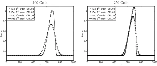
Figure 3: RMS Error against analytical solution for the flow of a Newtonian fluid over a moving granular bed between two infinite parallel planes: e p and e f stands for the

Dans le chapitre précédent, les équations régissant les phénomènes de transfert de masse, dans les différentes parties (canaux, GDL, catalyseurs et membrane) d’une pile à

High- resolution data of 2C velocity profiles collocated with concentration measurements have been obtained at the central line of the flume by using an ACVP (Acoustic Concentration

Que l’orbe incliné tourne d’un quart de cercle, le déférent d’un quart de cercle aussi, et le rotateur d’un demi-cercle dans le même temps ; alors l’inclinaison de

Goetze identified most of the mathematical texts in the Yale Babylonian Collection that Neugebauer later published (see for example YUL Goetze to Neugebauer 1942/02/04 in

frappé le secteur industriel durant [1989 et 1998] s’est traduite par une régression de 25,8% de l’indice de la production industrielle durant cette période, et une sous