Publisher’s version / Version de l'éditeur:
Vous avez des questions? Nous pouvons vous aider. Pour communiquer directement avec un auteur, consultez la première page de la revue dans laquelle son article a été publié afin de trouver ses coordonnées. Si vous n’arrivez pas à les repérer, communiquez avec nous à [email protected].
Questions? Contact the NRC Publications Archive team at
[email protected]. If you wish to email the authors directly, please see the first page of the publication for their contact information.
https://publications-cnrc.canada.ca/fra/droits
L’accès à ce site Web et l’utilisation de son contenu sont assujettis aux conditions présentées dans le site LISEZ CES CONDITIONS ATTENTIVEMENT AVANT D’UTILISER CE SITE WEB.
International Journal of Heat and Mass Transfer, 21, pp. 615-621, 1978
READ THESE TERMS AND CONDITIONS CAREFULLY BEFORE USING THIS WEBSITE. https://nrc-publications.canada.ca/eng/copyright
NRC Publications Archive Record / Notice des Archives des publications du CNRC :
https://nrc-publications.canada.ca/eng/view/object/?id=59ba5260-b509-4cb1-bc64-2cc77cb9b7bf
https://publications-cnrc.canada.ca/fra/voir/objet/?id=59ba5260-b509-4cb1-bc64-2cc77cb9b7bf
NRC Publications Archive
Archives des publications du CNRC
This publication could be one of several versions: author’s original, accepted manuscript or the publisher’s version. / La version de cette publication peut être l’une des suivantes : la version prépublication de l’auteur, la version acceptée du manuscrit ou la version de l’éditeur.
Access and use of this website and the material on it are subject to the Terms and Conditions set forth at
Efficient numerical technique for one-dimensional thermal problems
with phase change
~ i - 1 4
National Research
Conseil
national
a
77
1
l*
Council Canada
de recherches Canada
1 3
EFFICIENT NUMERICAL TECHNIQUE FOR
ONE-DIMENSIONAL THERMAL PROBLEMS WITH
PHASE CHANGE
Reprinted
from
International Journal of Heat and Mass Transfer VoL 21, 1978
p. 615
-
621DBR Paper No. 791
Division of Building Research
lnt, J. Heat Mass Transfer. Vol. 21, p p 615-621
@ Pergamon Press Ltd 1978. Printed in Great Britain
EFFICIENT NUMERICAL TECHNIQUE FOR
ONE-DIMENSIONAL THERMAL PROBLEMS
WITH PHASE CHANGE
L. E. GOODRICHNational Research Council, Canada, Division of Building Research, Geotechnical Section, Ottawa, Ontario, Canada K I A OR6
(Received 6 June 1977 and in revised form 21 September 1977)
Abstract-A new numerical scheme for one-dimensional heat flow problems with phase change is presented. The technique, which continuously monitors the progression of the phase interface, is unusual for the high
accuracy achieved without sacrifice to computing efficiency.
NOMENCLATURE heat capacity per unit volume;
thermal conductance coefficient, Fig. 1 ;
Gaussian elimination coefficients, equations (7a), (9a) ;
position of moving phase change interface ;
heat capacity coefficient, Fig. 1 ;
thermal conductivity ;
latent heat per unit volume;
Gaussian elimination coefficients, equations (7b), (9b);
temperature ;
time ;
depth.
terface. Because of certain numerical difficulties, these methods have not found favour in the past. The method now presented circumvents such difficulties and yields accurate solutions at low cost for these and other similar moving interface problems.
EXISTING METHODS
One-dimensional freezing or thawing with latent heat release ( + ) or absorption (-)at a fixed tempera- ture is described by the conditions
and
Greek symbols T(z, t) = Tj = constant (2
At, timestep; at the moving interface. The heat conduction equation Ax, space interval ;
AT, temperature range;
8, unfrozen moisture (volume basis). (3
Subscripts
A, apparent;
f , frozen or freezing;
i, node index ;
m, time step index;
N, node index for fixed boundary ; p, node index for element undergoing
phase change ; u, thawed or unfrozen.
FOR DESIGNING roadways and other engineering works in cold climates. as well as for more funda- mental studies of ground temperature regimes in nature, it is useful and often essential to have avail-
; able numerical techniques for calculating the depth of
frost or thaw penetration. For long-term com- putations involving many annual cycles, high numeri-
: cal efficiency is required in order to minimize costs. I
Road embankment calculations are usually concerned
I
with layered systems composed of materials thatI
possess a narrow freezing range. The most appropriate techniques for such cases are those that locate directly the position of the moving freezing or thawing in-applies in the frozen and unfrozen regions on either side of the moving phase boundary, due account being taken of differences in thermal properties.
Numerical treatments of phase change generally replace the moving boundary condition [equation (I)] by a latent heat source term added to the heat conduction equation to yield an apparent heat capacity formulation
with
C, = C, for T > Tj (4a) and
where
8 = 8(T, x) = unfrozen volumetric moisture content. In practice, the entire latent heat is usually associated with a small finite temperature range AT and equation
616 L. E. Go( (4b) is replaced by
C , = C f + L , / A T for T f - A T < T <
T,
C , = C f for T < T f - A T .Although apparent heat capacity formulations have the advantage of being simple to programme, the predicted phase change interface location, correspond- ing to the isotherm T =
T,,
advances in an unphysical oscillatory fashion and this is accompanied by distor- tion of the temperature profile in the region undergo- ing phase change. In order to hold errors within acceptable bounds the grid spacing in that region may have to be reduced substantially. This can, however, result in a situation in which the T,-isotherm moves across a grid element in less than one time step and the element latent heat contribution can be missed entirelv unless the time step also is reduced. Spatial resolution of the phase change interface location is poor, and this can be critical when dealing with layered problems with sharp contrast in thermal properties between neighbouring layers such as insulated road em- bankments. Inability to accommodate two phase change planes existing simultaneously within the same grid element can lead to errors in certain periodic thermal regime problems where coalescence is impor- tant. As well, in time-dependent boundary condition problems the error associated with oscillation can be cumulative. These difficulties are exacerbated when dealing with materials that possess a narrow freezing range or freeze at fixed temperature. Several different apparent heat capacity formulations have already been described [I-61.Only a limited number of formulations have been given that incorporate equation (1). Douglas and Gallie [7] and Kazemi and Perkins [8] describe methods that use variable time steps whose length must be found by nodal iteration, though the for- mulation uses explicit time differencing. A time de- pendent grid spacing scheme, also requiring nodal iteration, has been proposed by Heitz and Westwater [9] and Murray and Landis [lo]. Both methods are restricted to homogeneous media and are not suited to practical calculations.
It is also possible, and certainly preferable, to solve the system defined by equations (1)-(3) for the local position of the phase change plane within an element of fixed dimensions using fixed time steps. Crank [l 11 and Ehrlich [12] used higher order space differences for the phase change interface equation and this restricts the methbd to homogeneous media, at the same time necessitating intricate programming in order to move the interface across element boundaries. The formulation of Meyer et al. [13] is a lumped- parameter scheme using finite differences for the time dimension only. It is flexible, but a considerable amount of computation is required at each time step. Hwang [I41 presented a scheme in which an equiva- lent of equation (1) can be used to estimate an elemental latent heat source term for inclusion in a two-dimensional finite-element formulation. The la- tent heat is considered to be distributed over the
element in a manner similar to that of apparent heat capacity formulations, and the phase change interface location is not followed continuously as such. The initial Tf-isotherm position is, instead, estimated at each time step by linear interpolation of the cor- responding temperature profile. In addition, the non- linearity associated with the phase change equation and hence the necessity of using nodal iteration for solution is eliminated by using a forward difference approximation for the latent heat contribution. Al- though these approximations can be justified on practical grounds for two-dimensional problems, the resulting numerical accuracy is not so high as could otherwise be achieved.
Many of the drawbacks associated with these me- thods can be circumvented, and it is the purpose of this paper to describe a technique capable of locating the phase change interface in one-dimensional layered systems accurately and efficiently. The method uses a centred-difference formulation with solution by simple Gaussian elimination at ordinary nodes. The element undergoing phase change is treated by a technique that continuously follows the position of the moving phase change interface by means of a formulation that maintains the non-linear character of the problem without requiring costly nodal iterations for solution.
PROPOSED NUMERICAL TECHNIQUE FOR PHASE CHANGE AT FIXED TEMPERATURE The centred time difference equation for layered systems can be written
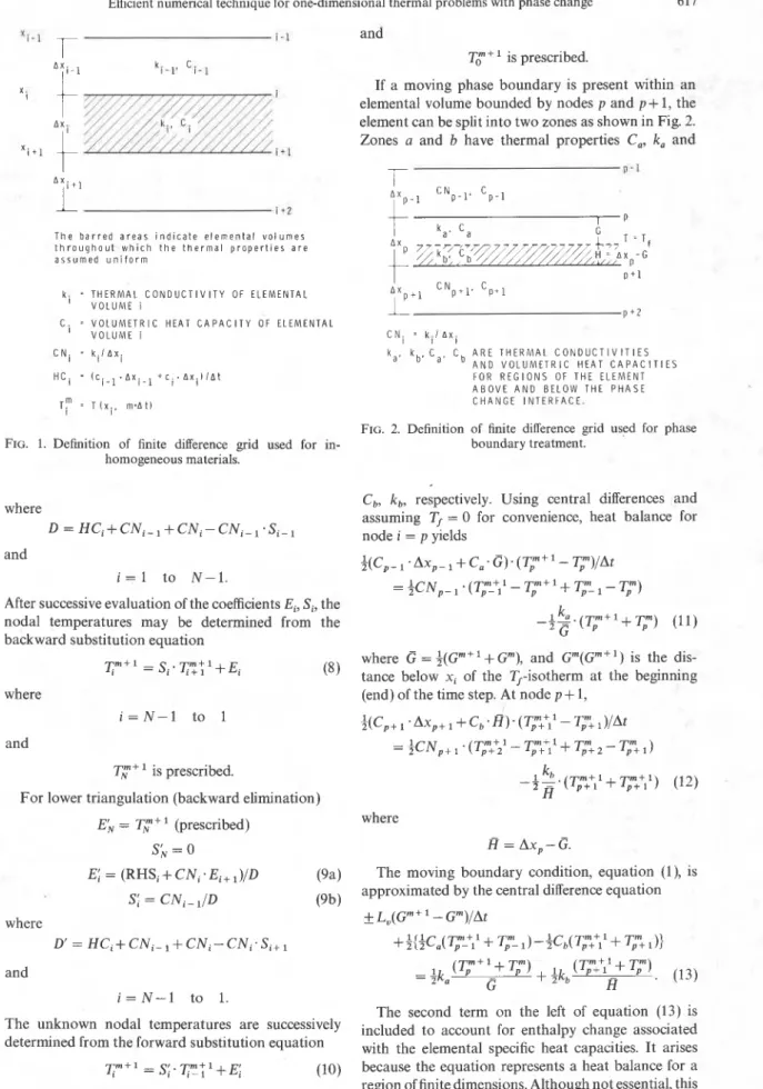
where i and rn are space and time indices, respectively. The heat capacity coefficients HC and conductance coefficients C N are defined in Fig. 1. Rearranging, the equation may be cast in the form
- C N i - 7;?!:'
+
( H C i + C N , - I+
C N , )T m f
- C N i.7;m+:
= RHSi (6) whereRHSi = C N i - 1 . IT,"!!
With boundary temperatures prescribed at nodes i = 0 and i = N corresponding to the upper and lower surfaces, respectively, the unknown temperatures 7;"+', 1 < i < N - 1 can be found by solving the system of equations represented by equation (6) using Gaussian elimination. Two equivalent formulations are possible. Upper triangulation (forward elim- ination) yields
I Efficient numerical technique for one-dimensional thermal problems with phase change 617
i - I and
T," + is prescribed.
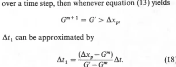
If a moving phase boundary is present within an
elemental volume bounded by nodes p and p + 1, the
element can be split into two zones as shown in Fig. 2.
Zones a and b have thermal properties C,, k, and
-
I P - 1 A X . I 1.2 1 P T h e b a r r e d a r e a s i n d i c a t e e l e m e n t a l v o l u m e s G t h r o u g h o u t w h i c h t h e t h e r m a l p r o p e r t i e s a r e &-,7 = T f a s s u m e d u n i f o r m H = A x - G /'/ P P + l k i = T H E R M A L C O N D U C T I V I T Y O F E L E M E N T A L V O L U M E i C i = V O L U M E T R I C H E A T C A P A C I T Y O F E L E M E N T A L P t Z V O L U M E i C N . = k i l A x i C N i = k . l d x . I I k a , k b , C a , C b A R E T H E R M A L C O N D U C T I V I T I E S A N D V O L U M E T R I C H E A T C A P A C I T I E S H C ~ = ( c ~ - ~ . A x ~ - ~ + c . . A X . I I A ~ I I F O R R E G I O N S O F T H E E L E M E N T A B O V E A N D B E L O W T H E P H A S E TI" = ~ ( x . . m . ~ t ) C H A N G E I N T E R F A C E .FIG. 2. Definition of finite difference grid used for phase
FIG. 1. Definition of finite difference grid used for in- boundary treatment. homogeneous materials.
C,, k,, respectively. Using central differences and where
assuming T, = 0 for convenience, heat balance for
D = HCi+CNi-l+CNi-CNi-l.Si-l node i = p yields
and + ( C p - l . A ~ p - l +Ca.G).(Tpm+ l - Y ) / A t
i = l to N-1. = ~ c N , - ~ . ( ~ + ~ ~ - ~ ~ ~ + T , " _ ~ - ~ )
After successive evaluation of the coefficients Ei, S , the
nodal temperatures may be determined from the ---
backward substitution equation G
~ m + l =
si.
~ m + ; l + ~ ~ where G = $(Gmf' +
Gm), and Gm(Gm+ ') is the dis-tance below xi of the TI-isotherm at the beginning
where (end) of the time step. At node p
+
1,i = N - 1 to 1 $ ( C , + I . ~ X , + ~ + ~ ~ ' ~ ) . ( ~ " + ~ I ~ - ~ + I ) / ~ ~
and = ~ C N , + , ~ ( T , " ~ ~ ~ ~ - T ~ " , ~ ~ + T ~ " , ~ - T ~ " , ~ )
T,"+ l is prescribed.
.
:
4
-
k,( ~ ' " + l
H p + 1
+
Tpm:ll) (12) For lower triangulation (backward elimination)~1 - - ~ m + l (prescribed) where
Sk = 0 H = AX, - G.
Ei = (RHS,
+
CN, . Ei+ ,)ID (9a) The moving boundary condition, equation (I), is(9'3) approximated by the central difference equation
Si = CN, - ,ID where ) L,(Gm +
'
- Gm)/At D' = HCi+CNi-l+CNi-CNi.Si+l + + { + C , ( c l+
Td"_ l)-$Cb(T,m:ll+
Tpm+ and = $ka G+
$kb H . (13) i = N - 1 to 1.The second term on the left of equation (13) is
The unknown temperatures are included to account for enthalpy change associated
determined from the forward substitution equation with the elemental specific heat capacities, arises
rm+l
=s;.IT,'"~+E; (10) because the equation represents a heat balance for aregion of finite dimensions. Although not essential, this
where additional term does improve accuracy, particularly
specific heat capacity terms. Heat transfer at the over a time step, then whenever equation ( 1 3 ) yields remaining ordinary nodes is described by equation
(5). As Gm+' is ' not known explicitly, the system
including equations ( 5 ) and (11)-(13) is non-linear.
Introduction of nodal iteration can, however, be Can be by avoided by judicious use of both forward and back-
( A X , - G m )
ward Gaussian elimination. A t , = At.
G'-Gm ( 1 8 )
From the forward elimination formula, equation (7),
the coefficients Ei, Si can be determined successively for Nodal temperatures are updated using the partial time
i = 1 to i = p - 1. For node i = p, equation ( 1 1 ) leads step At,, after which displacement of the phase change
L"
+%!!-
C N p - l At E, = C . G k, ( 1 4 ) A x p l+
+
--
+
C N , - , ( I - S p - , ) C,-,.-
At At Gand from equation (8)
qm+'
= S p . T f + E Por. since
Similarly, the backward elimination technique, equation (9) and ( l o ) , for the region below the phase plane gives
where, following equation ( 1 2 )
and the coefficients Ei, SI are calculated successively from equation (9) with i = N - 1 to i = p + 2 .
It should be noted that in both equations ( 1 4 ) and
( 1 7 ) all terms on the RHS are known explicitly except
Gm+ 1
. The introduction of forward elimination above, and backward elimination below, the moving boun- dary has the effect of isolating the non-linearity associated with the moving interface. Equation ( 1 3 ) combined with equations ( 1 5 ) and ( 1 6 ) is a non-linear, ordinary difference equation whose solution yields
Gm+' and the nodal temperatures
qmfl
andVl1
simultaneously. The remaining nodal temperatures can be determined from the appropriate backward or forward substitution equation, without recourse to nodal iteration. Equations (13), ( 1 5 ) and ( 1 6 ) can be solved by any convenient method. The Secant method is appropriate and converges after four or five iter- ations at most. Simple iteration is also satisfactory.
To complete the numerical formulation it is nec- essary to provide a means of permitting the phase change interface to move across an element boundary. This may be accomplished by splitting the time step.
At = A t , + A t ,
where
plane within the neighbouring element i = p + 1 is evaluated for the remaining interval At,; the nodal temperatures are then updated to their final values
y+'.
An analogous procedure is used whenever G' < 0 .VERIFICATION OF THE METHOD
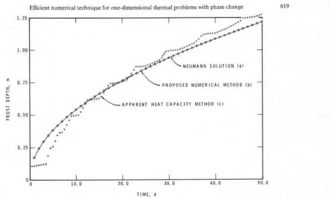
Figure 3 compares an analytical and two numerical solutions for a simplified Neumann freezing problem. Comparison is based on frost penetration and it may be noted that this offers a more sensitive test of the quality of the method than does the more usual comparison of temperature profiles. The following parameter values were chosen:
T ( x , 0 ) = =
+
2°CT ( 0 , t ) = T,",,, = - 10°C t > 0 T ( a 3 , t ) = t 2 0
k, = k t = 2 W / m . K
L, = 100 MJ/m3.
Thermal conductivities and heat capacities were as- sumed to be identical in the frozen and thawed regions
A t , = time interval required to move the Tf-isotherm to ensure that differences in results obtained by the
Efficient numerical technique for one-dimensional thermal problems with phase change
A P P A R E N T H E A T C A P A C I T Y M E T H O D ( c )
1
T I M E , d
FIG. 3. Comparison of two numerical methods vs analytic solution for frost penetration. made in the treatment of latent heat. Curve (a) shows
the frost penetration calculated from the analytical solution ; curve (b) was computed using the numerical method presented here. For comparison, curve ( c ) was calculated using an apparent heat capacity for- mulation assuming a freezing range of 0.5 K. A Crank-Nicholson formula was used with thermal properties updated at each time step. In both cases precautions were taken to eliminate the starting error associated with the step-function surface condition. Results for the author's method were calculated using a grid spacing and time step
A x = 0.25 m
At = 1 day
while the apparent heat capacity formulation required
A x = 0.125 m
At = 0.25 day.
This represents nearly an eight-fold increase in com- putation time.
It may be seen that the present method follows very closely the true frost penetration at all times, with no tendency to oscillate. Accuracy is such that results are essentially indistinguishable from those of the analytic solution. The relative crudeness of the apparent heat capacity method is evident.
A second comparison is presented in Fig. 4, in which the problem is similar to that of Fig. 3 except for the thermal properties, which were taken as
Degeneration of the numerical results is minimal. Although not shown, the relative performance of the apparent heat capacity formulation would have been even worse in this case than in the previous one inasmuch as the solution oscillations are no longer compensated symmetrically.
DISCUSSION
The proposed method offers a number of advan- tages when compared with existing techniques. The rather exceptional accuracy inherent in the for- mulation is obtained with no loss of efficiency and, in fact, computation times are essentially the same as those required for the central difference calculation at the ordinary nodes. The method is completely flexible, and layered systems with sharp contrasts in thermal properties, either between layer boundaries or as- sociated with change of phase, can be handled ef- ficiently without degradation of solution accuracy. Because the solution accurately tracks the true frost penetration at all times, high accuracy can be main- tained even in problems with rapidly changing surface boundary conditions. The latent heat formulation does not in itself impose restrictions on the size of grid spacing or time step. These are limited only by the usual truncation error associated with the Crank-Nicholson equations for the ordinary nodes.
The latent heat treatment, as described, is restricted to problems with a single freezing or thawing front. Situations involving more than one phase interface can occur,'for example, in the study of annual ground thermal regimes. The combined backward and for- ward Gaussian elimination solution technique cannot be used to avoid nodal iteration if two phase planes are present. In many practical cases, however, tempera- tures in the zone between the two phase interfaces
FIG. 4 . Calculated frost depth comparison-non-constant thermal properties. rapidly approach the freezing point. Under these
conditions heat flow is small compared with values outside the zone and can be ignored. A single-sided formulation of the method can then be used for each phase change plane separately, and in this way nodal iteration can be avoided. In addition, coalescence of the phase change planes can be followed even when both interfaces occur within the same element. This approach was used in a programme developed to study the effects of snow cover on ground thermal regimes. Complete FORTRAN programmes based on earlier versions of the formulation have been given
[15-171. If nodal iteration cannot be tolerated for problems with multiple phase interfaces, where the isothermal assumption cannot be made or where thermal properties are very strong functions of tem- perature, it may be desirable to reformulate the method using a three time level scheme. This approach is to be considered in a future study.
CONCLUSION
A new numerical technique for treating one- dimensional problems with phase change has been developed. The numerical accuracy of the method is much superior to that of the apparent heat capacity formulation. The solution technique retains the non- linearity associated with the moving phase boundary without requiring costly nodal iteration. The resulting high efficiency is further enhanced by the insensitivity of the method to size of grid spacing and time step.
Comparison with the analytical solution for a simplified problem showed that the numerical method yields results closely following those for analytically calculated frost penetration. In contrast with the apparent heat capacity formulation, the solution
showed no tendency to oscillate and the high accu- racy achieved was maintained at all times. Compari- son with the analytic solution for a freezing problem with phase dependent thermal properties showed no significant deterioration of accuracy. Similar perform- ance can be expected with layered systems or problems with rapidly changing boundary conditions.
Acknowledgement-This paper is a contribution from the Division of Building Research, National Research Council of Canada and is published with the approval of the Director of the Division.
REFERENCES
1. C . Bonacina, G. Comini, A. Fasano and M. Primicerio, Numerical solution of phase-change problems, Int. J.
Heat Mass Transfer 16,1825-1832 (1973).
2. B. J . Dempsey and M. R. Thompson, A heat-transfer model for evaluating frost action and temperature- related effects in multilayered pavement systems, H.R.R.
342,39-56 (1970).
3. A. K . Fleming, The numerical calculation of freezing
processes, Presented at 13th International Institution of
Refrigeration Congress, Washington, September 1971.
4 . D. M. Ho, M. E. Harr and G. A. Leonards, Transient temperature distribution in insulated pavements- predictions vs observations, Can. Geotech. J17,275-284
(1970).
5 . Y . Nakano and J. Brown, Effect of a freezing zone of finite width on the thermal regime of soils, Water Resources
Res. 7 ( 5 ) , 1226-1233 (1971).
6 . P. H. Price and M. R. Slack, The effect of latent heat on numerical solutions of the heat flow equation, Br. J. Appl.
Phys. 5,285-287 (1954).
7 . J . Douglas and T. Gallie, On the numerical integration of a parabolic differential equation subject to a moving boundary condition, Duke Math. J1 22(4), 557-571
(1955).
8 . H. Kazemi and T. K. Perluns, Mathematical model of freeze-thaw cycles beneath drilling rigs and production platforms in cold regions, J. Petrol. Technol. 381-390
Efficient numerical technique for one-dmensional thermal problems with phase change 62 1
9. W. L. Heitz and J. W. Westwater, Extension of the numerical method for melting and freezing problems, Int.
J . Heat Mass Transfer 13(8), 1371-1375 (1970). 10. W. D. Murray and F. Landis, Numerical and machine
solutions of transient heat conduction problems involv- ing melting or freezing. Part 1-Method of analysis and sample solutions, J . Heat Transfer 81, 106-112 (1959).
11. J . Crank, Two methods for the numerical solution of moving boundary problems in diffusion and heat flow, Q.
J l Mech. Appl. Math. 10,220-231 (1957).
12. L. W. Ehrlich, A numerical method of solving a heat flow problem with moving boundary, J. Ass. Comput. Mach.
5(2), 161-176 (1958).
13. G. M. Meyer, H. M. Keller and E. J. Couch, Thermal
model for roads, airstrips and building foundations in permafrost regions, J. Can. Petrol. Technol., April-June,
13-25 (1972).
14. C. T . Hwang, A thermal analysis for structures on permafrost, Can. Geotech. J19,33 (1972).
15. L. E. Goodrich, A one-dimensional numerical model for geothermal problems, Nat. Res. Council of Canada, Div. Bldg. Res., NRCC 14123 (1974).
16. L. E. Goodrich, FORTRAN IV program for general one- dimensional geothermal problems, Nat. Res. Council of Canada, Div. Bldg. Res., C P 39 (1974).
17. L. E. Goodrich, A numerical model for assessing the influence of snow cover on the ground thermal regime, Ph.D. Thesis, McGill University (1976).
TECHNIQUE NUMERIQUE PERFORMANTE POUR DES PROBLEMES THERMIQUES MONODIMENSIONNELS AVEC CHANGEMENT DE PHASE Rkume-On prtsente une nouvelle procidure nurnerique pour traiter les problemes thermiques mono- dimensionnels avec changement de phase. La technique qui suit continClment la progression de l'interface de changement de phase est remarquable par sa grande precision obtenue sans sacrifier a la performance
de calcul.
WIRKSAMES NUMERISCHES VERFAHREN FUR EINDIMENSIONALE
WARMEUBERTRAGUNGSPROBLEME MIT PHASENWECHSEL
Zusammenfassung-Es wird ein neues numerisches Verfahren fiir eindimensionale Wiirmeubertragungsprobleme mit Phasenanderung vorgestellt. Bei diesem Verfahren wird der Ort der Phasengrenzflache bei jedem Zeitschritt explizit bestimmt. Der Aufsatz enthalt auI3erdem ein Losungsverfahren fur das Gleichungssystem, das Iterationen in jedem Gitterpunkt vermeidet. Daraus resultiert ein Rechenverfahren, das zugleich numerisch
wirkungsvoll und ungewohnlich genau ist.
~HHOTBUR - B pa6ol.e ITpenCTaBneH ~0Bblfi Y E T C ~ ~ H H ~ I ~ MeTOn PeIlIeHUH OnHOMepHblX 3anaY
~ e n n o o 6 ~ e ~ a npu @aso~brx npeBpawenHnx, nosaonslowwt aenpepbmao onpenenmb nonoxeaue nepe~eualotuefics rpaauubr pasnena @as. Aaaabrfi Meron 06nanae.r ebrcorofi TOYHOCT~EO u