HAL Id: hal-01157388
https://hal.inria.fr/hal-01157388
Submitted on 28 May 2015
HAL is a multi-disciplinary open access
archive for the deposit and dissemination of
sci-entific research documents, whether they are
pub-lished or not. The documents may come from
teaching and research institutions in France or
abroad, or from public or private research centers.
L’archive ouverte pluridisciplinaire HAL, est
destinée au dépôt et à la diffusion de documents
scientifiques de niveau recherche, publiés ou non,
émanant des établissements d’enseignement et de
recherche français ou étrangers, des laboratoires
publics ou privés.
Comparison of the MATSuMoTo Library for Expensive
Optimization on the Noiseless Black-Box Optimization
Benchmarking Testbed
Dimo Brockhoff
To cite this version:
Dimo Brockhoff. Comparison of the MATSuMoTo Library for Expensive Optimization on the Noiseless
Black-Box Optimization Benchmarking Testbed. Congress on Evolutionary Computation (CEC 2015),
May 2015, Sendai, Japan. �hal-01157388�
Comparison of the MATSuMoTo Library for
Expensive Optimization on the Noiseless Black-Box
Optimization Benchmarking Testbed
Dimo Brockhoff
Inria Lille - Nord Europe, DOLPHIN team
Email: [email protected]
Abstract—Numerical black-box optimization problems occur
frequently in engineering design, medical applications, finance,
and many other areas of our society’s interest. Often, those
prob-lems have expensive-to-calculate objective functions for example
if the solution evaluation is based on numerical simulations.
Starting with the seminal paper of Jones et al. on Efficient
Global Optimization (EGO), several algorithms tailored towards
expensive numerical black-box problems have been proposed.
The recent MATLAB toolbox MATSuMoTo (short for MATLAB
Surrogate Model Toolbox) is the focus of this paper and is
benchmarked within the Black-box Optimization Benchmarking
framework BBOB. A comparison with other already previously
benchmarked algorithms for expensive numerical black-box
op-timization with the default setting of MATSuMoTo highlights
the strengths and weaknesses of MATSuMoTo’s cubic radial
basis functions surrogate model in combination with a Latin
Hypercube initial design in the range of 50 times dimension many
function evaluations.
I. I
NTRODUCTION
Numerical black-box optimization problems, i.e., problems
with continuous variables but without the availability of
deriva-tives, have to be solved frequently in many businesses these
days. The number of available function evaluations is thereby
often restricted to about 10 to 1000 times the search space
dimension DIM (expensive setting) as a typical evaluation of
the objective function can take several minutes or even hours
of (already parallelized) computation time.
A state-of-the-art approach to tackle expensive optimization
problems is to build a so-called surrogate model of the
objective function (based on already evaluated search points)
and to use this easier-to-evaluate surrogate model to predict
good candidate solutions. Several surrogate-assisted (or
model-based) algorithms for expensive numerical black-box
opti-mization problems exist which mainly differ in the type of the
underlying model of the objective function (local vs. global,
Erratum: The statement “MATSuMoTo often scales linearly or
quadrat-ically with the problem dimension for solved problems while the expected
running time for RANDOMSEARCH explodes exponentially.” in the original
paper was wrong and has now been replaced by “For the solved problems,
MATSuMoTo often scales linearly or quadratically relative to the best
algo-rithm of BBOB 2009 while the expected running time for RANDOMSEARCH
always explodes exponentially.”
This is an updated version of the original paper, published at IEEE
Congress on Evolutionary Computation (CEC 2015). The original publication
is available at http://ieeexplore.ieee.org.
quadratic model, Kriging, radial basis functions, etc.) and the
way this model is used for optimization (for example wrt. the
criterion for selecting candidate solutions). The criterion for
choosing new candidate solutions (to be evaluated on the true,
expensive objective function) is known under different names
such as “figure of merit” or “infill criterion”.
The probably most known approach to expensive numerical
black-box optimization is the Efficient Global Optimization
algorithm (EGO) from the seminal paper by Jones et al. [1].
Here, multivariate Gaussian processes are used as surrogate
models and the expected improvement as infill criterion.
The recently proposed SMAC-BBOB [2] is a similar
ap-proach to EGO and uses the same surrogate models and
infill criterion as EGO. In comparison to EGO, however,
SMAC-BBOB uses the specific “noise-free isotropic Matern
kernel and no initial design” [2]. Furthermore, the optimization
algorithms DIRECT and CMA-ES are used to optimize the
expected improvement criterion instead of the
branch-and-bound approach of the original EGO.
A local meta-model based version of the CMA-ES
algo-rithm itself, denoted by lmm-CMA-ES, has been proposed
by Kern et al. [3] and was later slightly improved [4]. As
its original version CMA-ES, it samples in each iteration λ
candidate solutions from a multivariate normal distribution
which itself is updated based on the ranking of the candidate
solutions’ objective function values. In the lmm-CMA-ES, a
local quadratic surrogate model is build around each candidate
solution to predict a ranking. Iteratively, only a small portion of
the candidate solutions is then evaluated on the true objective
function until the (updated) ranking does not change anymore.
Another variant of the original CMA-ES algorithm which
uses surrogates is the so-called IPOPsaACM algorithm [5].
On top of a variant of CMA-ES that uses a ranking support
vector machine as surrogate model, the IPOPsaACM proposes
a heuristic that adapts both the number of function evaluations,
within which the surrogate model is kept constant, and the
surrogate’s model parameters itself.
Last, let us mention the algorithm NEWUOA by Powell [6],
[7] which is not specifically designed for solving expensive
optimization problems but also builds a (global) quadratic
model of the objective function in each iteration and, thus,
should be considered as a baseline in each comparison of
optimizers for expensive numerical black-box optimization
problems. Instead of using quadratically many solutions to fit
the quadratic surrogate model of NEWUOA, typically only
linearly many solutions are used to define the surrogate.
Min-imizing the Frobenius norm of the second derivative matrix
of the model changes in each iteration then makes up for the
remaining freedom of the quadratic model.
In order to find out which of the many available optimization
algorithms performs best on certain classes of functions,
benchmarking in terms of numerical experiments is the
com-pulsory path to assess performance of optimizers quantitatively
and to understand weaknesses and strengths of each algorithm.
To facilitate this tedious task, the Comparing Continuous
Optimizers platform (COCO) has been developed and used
to create the Black-box Optimization Benchmarking (BBOB)
test suite [8]. It provides all necessary code for running
the experiments on 24 well-known and -understood noiseless
test functions, the collection of data, up to the automated
postprocessing of them—including the generation of data
profiles, scaling graphs, and tables. In the beginning of 2015,
around 120 different algorithms have been benchmarked with
the COCO/BBOB framework and the corresponding data sets
are available online at http://coco.gforge.inria.fr/. However, the
data collection is by far not exhaustive and in particular in the
expensive setting (between 10 ⋅ DIM and 1000 ⋅ DIM function
evaluations) does not cover many different algorithm classes.
Our Contributions:
This paper will, therefore, benchmark
a recently proposed approach to expensive optimization, the
MATLAB Surrogate Model Toolbox (MATSuMoTo) [9], [10],
and compare its performance on the BBOB noiseless testbed
with other above mentioned algorithms. The MATSuMoTo
library allows to choose from a variety of different initial
designs, surrogate models, and criteria for the choice of new
candidate solutions and a previous benchmarking of the
avail-able variants has established a default setting which is based
on cubic radial basis functions (RBFs) as surrogate models
[10]. Since cubic RBFs have not been used as surrogates in
any algorithm previously compared on the expensive BBOB
testbed, we turn our attention here to the comparison of
this default setting of MATSuMoTo with other previously
benchmarked algorithms for expensive optimization.
II. T
HE
MATS
U
M
O
T
O
L
IBRARY AND THE
B
ENCHMARKED
D
EFAULT
A
LGORITHM
S
ETTING
The MATLAB Surrogate Model Toolbox (MATSuMoTo)
is an optimization toolbox for “computationally expensive,
black-box, global optimization problems that may have
con-tinuous, mixed-integer, or pure integer variables” [9]. Various
surrogate models, initial experimental design strategies and
infill criteria are available. Also mixtures of surrogate models
as employed and compared in [10] can be used. We here
restrict ourselves to the continuous optimization part of the
toolbox.
Several parameters have to be specified by the user when
using MATSuMoTo, concretely the optimization problem, the
maximum number of allowed expensive function evaluations,
the surrogate model type, the sampling strategy, the type of
the initial experimental design, the number of points in the
initial experimental design, and the number of points to be
selected in each iteration for the expensive function
evalua-tions. Optionally, specific points to be included in the initial
experimental design can be specified. As the default setting of
MATSuMoTo will be chosen by most new users of the toolbox
as a starting point, we compare this default setting as a baseline
version of MATSuMoTo within the BBOB framework. The
default setting has been chosen based on a previous extensive
comparison of all of MATSuMoTo’s components. The default
setting of MATSuMoTo corresponds to using cubic radial
basis functions as surrogate model, randomized sampling by
local perturbation of the best point found so far together with
additional points uniformly selected from the whole variable
domain as sampling strategy, a Latin Hypercube sampling as
initial experimental design with 2 ⋅ (DIM + 1) samples, and
one new sample per iteration. Only the stopping criterion was
set differently than the default, namely to 50 ⋅ DIM instead of
20 ⋅ DIM.
Slight modifications had to be done to the original
MAT-SuMoTo code to be able to connect it to the BBOB framework.
The main change is that no parallel evaluations are performed
anymore via MATLAB’s Parallel Computing toolbox but
in-stead the natural parallel evaluations of BBOB are used. As
basis for our experiments, the online available MATSuMoTo
version of April, 8, 2014 has been used. The source code for
the BBOB experiments will be available via http://coco.gforge.
inria.fr/doku.php?id=cec-bbob-2015-results.
III. E
XPERIMENTAL
S
ETTING
A. Compared Algorithms
Besides the above described default setting of
MAT-SuMoTo, several algorithm data sets from the COCO/BBOB
web page have been included in the comparison: NEWUOA
[7], SMAC-BBOB [2], lmm-CMA-ES [4], IPOPsaACM [5]
and pure random search [11]. The default MATSuMoTo
opti-mizer has been run for 50 ⋅ DIM function evaluations.
B. CPU Timing of the Default MATSuMoTo
In order to evaluate the CPU timing of the MATSuMoTo
library, we have run the algorithm with default settings on the
function f
8
with restarts for at least 30 seconds and until a
maximum budget equal to 50 ⋅ DIM is reached. The code was
run on an Intel(R) Core(TM)2 Quad Q6600 CPU @ 2.40GHz
with 1 processor and 4 cores. The time per function evaluation
for dimensions 2, 3, 5, 10, and 20 equals 0.058, 0.12, 0.26,
0.89, and 2.9 seconds respectively.
C. BBOB-related Settings
Results from experiments according to [8] on the functions
given in [12] are presented in Figures 1, 2 and 3 and in Tables I
and II. The expected running time (ERT) therein depends on
a given target function value, f
t
=
f
opt
+
∆f , and is computed
over all relevant trials as the number of function evaluations
executed during each trial while the best function value did not
reach f
t
, summed over all trials and divided by the number of
trials that actually reached f
t
[8], [13]. Statistical significance
is tested with the rank-sum test for a given target ∆f
t
using,
for each trial, either the number of needed function evaluations
to reach ∆f
t
(inverted and multiplied by −1), or, if the target
was not reached, the best ∆f -value achieved, measured only
up to the smallest number of overall function evaluations for
any unsuccessful trial under consideration.
IV. D
ISCUSSION OF THE
R
ESULTS
When looking at the benchmarking results in Figs. 1, 2, and
3 and in Tables I and II, four main observations can be made:
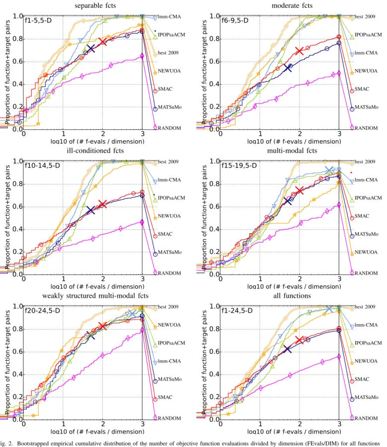
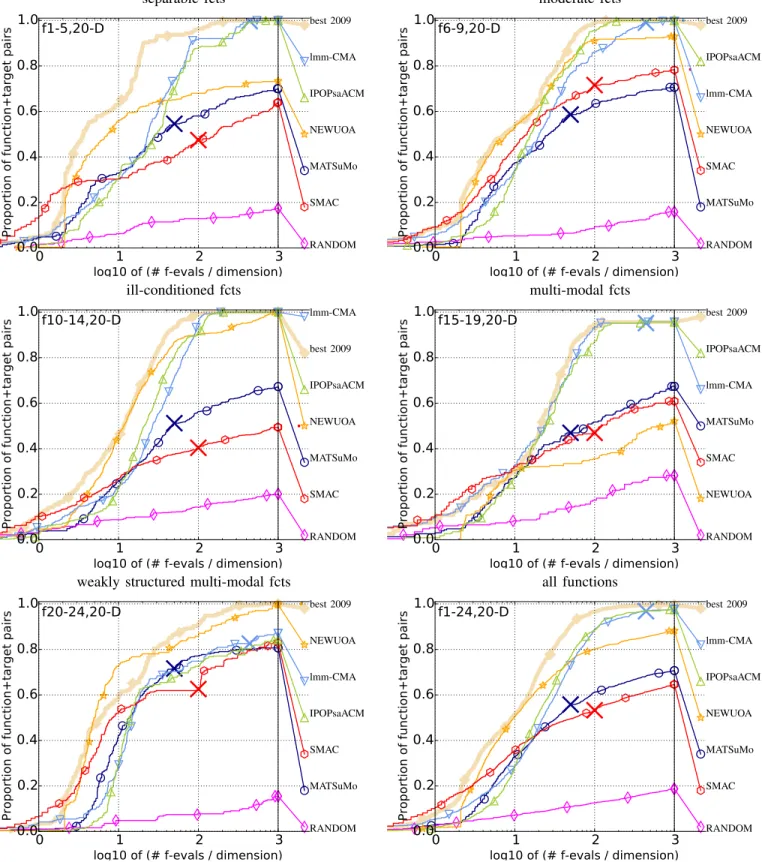
Scaling with Dimension:
Over all problems, MATSuMoTo
ranges in performance between RANDOMSEARCH and the
other surrogate model based algorithms when looking at the
expensive scenario of 10 ⋅ DIM function evaluations (Fig. 1).
For the solved problems, MATSuMoTo often scales linearly
or quadratically relative to the best algorithm of BBOB 2009
while the expected running time for RANDOMSEARCH
always explodes exponentially.
Solvable Instances:
In 20-D (5-D), MATSuMoTo does
not solve nine (three) of the 24 noiseless BBOB functions
to the precision of the BBOB-2009 reference algorithm after
10⋅DIM function evaluations. Surprisingly, the sphere function
cannot be solved to a precision of 10
−8
within 50 ⋅ DIM
evaluations—not even in 2-D. The only algorithms in the
comparison for which this is also the case in 5-D and
20-D, are RANDOMSEARCH and SMAC-BBOB. Preliminary
experiments with other MATSuMoTo settings show similar
results but a thorough investigation remains future work.
Strong Performances of MATSuMoTo:
The best relative
per-formances of MATSuMoTo can be observed on the functions
f
15
(Rastrigin) and f
21
(Gallagher’s 101 Peaks) in 5-D and on
f
21
and f
22
(Gallagher’s 21 Peaks) in 20-D—providing the
best performances among the compared algorithms. For the
20-D functions f
21
and f
22
and the largest expensive budget
of 50 ⋅ DIM, MATSuMoTo is even outperforming the best
algorithm of BBOB-2009. For smaller budgets than 50 ⋅ DIM
and in 5-D, also the results on f
2
, f
6
, and f
16
are competitive
and MATSuMoTo sometimes outperforms the best
BBOB-2009 algorithm. None of the results is statistically significant.
Overall Comparison with Other Surrogate-Assisted
Opti-mizers:
When compared on the data profiles of Fig. 2
and 3, it appears that the default MATSuMoTo optimizer
is always dominated by some other algorithm. Moreover,
the combination of the three algorithms SMAC-BBOB (for
very low budgets below ≈ 3 ⋅ DIM function evaluations),
NEWUOA (for medium budgets), and lmm-CMA-ES (for
relatively large budgets of ≥ 30 ⋅ DIM evaluations) build a
good portfolio that constructs the upper envelope over all
compared algorithms for almost all problem groups. Adding
IPOPsaACM to the portfolio further improves performance
slightly on the moderate function group for the most difficult
targets.
V. C
ONCLUSIONS
The MATLAB Surrogate Model Toolbox (MATSuMoTo)
has been taken out-of-the-box in its default setting and was
compared with other model-building algorithms of the
avail-able BBOB algorithm data collection on the 24 noiseless test
functions of the BBOB suite. It turns out that MATSuMoTo
shows comparable results over most functions: though in
di-mension 20, nine functions cannot be solved to comparatively
high precision, on the two Gallagher functions (f
21
and f
22
),
the best BBOB-2009 algorithm is outperformed for the largest
expensive budgets (all results not statistically significant).
Overall, MATSuMoTo is a practically interesting
optimiza-tion toolbox due to its flexibility and availability in MATLAB.
However, other available algorithms that outperform its default
setting exist and it remains open to investigate more carefully
the impact of the other options offered by the framework on
the BBOB test suite, similar to the comparison in [10]. In
particular, the influence of the initial design, the used surrogate
model and the employed infill criterion in surrogate-assisted
optimization algorithms should be investigated further.
A
CKNOWLEDGMENT
This work was supported by the French National Research
Agency under grant ANR-12-MONU-0009 (NumBBO), the
JSPS funded project “Global Research on the Framework of
Evolutionary Solution Search to Accelerate Innovation” and
Inria’s ´
Equipe Associ´ee “s3-bbo”. Figures, Tables, and part of
Sec. III stem from the open-source platform COCO [8].
R
EFERENCES
[1] D. R. Jones, M. Schonlau, and W.-J. Welch, “Efficient Global
tion of Expensive Black-Box Functions,” Journal of Global
Optimiza-tion, vol. 13, no. 4, pp. 455–492, 1998.
[2] F. Hutter, H. Hoos, and K. Leyton-Brown, “An Evaluation of
Se-quential Model-Based Optimization for Expensive Blackbox
Func-tions,” in GECCO workshop on Black-Box Optimization Benchmarking
(BBOB’2013).
ACM Press, 2013, pp. 1209–1216.
[3] S. Kern, N. Hansen, and P. Koumoutsakos, “Local Meta-models for
Optimization Using Evolution Strategies,” in Parallel Problem Solving
from Nature (PPSN IX).
Springer, 2006, pp. 939–948.
[4] A. Auger, D. Brockhoff, and N. Hansen, “Benchmarking the
Lo-cal Metamodel CMA-ES on the Noiseless BBOB2013 Test Bed,” in
GECCO (Companion) workshop on Black-Box Optimization
Bench-marking (BBOB’2013).
ACM, 2013, pp. 1225–1232.
[5] I. Loshchilov, M. Schoenauer, and M. Sebag, “Black-box
Optimiza-tion Benchmarking of IPOP-saACM-ES and BIPOP-saACM-ES on the
BBOB-2012 Noiseless Testbed,” in GECCO (Companion) workshop on
Black-Box Optimization Benchmarking (BBOB’2009).
New York, NY,
USA: ACM, 2012, pp. 175–182.
[6] M. J. D. Powell, “The NEWUOA Software for Unconstrained
Op-timization Without Derivatives,” Department of Applied Mathematics
and Theoretical Physics, Cambridge University, Tech. Rep. DAMTP
2004/NA05, Nov. 2004.
[7] R. Ros, “Benchmarking the NEWUOA on the BBOB-2009 Function
Testbed,” in GECCO (Companion) workshop on Black-Box Optimization
Benchmarking (BBOB’2009).
ACM, 2009, pp. 2421–2428.
[8] N. Hansen, A. Auger, S. Finck, and R. Ros, “Real-parameter black-box
optimization benchmarking 2012: Experimental setup,” INRIA, Tech.
Rep., 2012. [Online]. Available: http://coco.gforge.inria.fr/doku.php?id=
cec-bbob-2015-downloads
[9] J. M¨uller, “MATSuMoTo: The MATLAB Surrogate Model Toolbox For
Computationally Expensive Black-Box Global Optimization Problems,”
ArXiv e-prints, Apr. 2014.
2
3
5
10
20
40
0
1
2
3
4
5
6
target RL/dim: 10
1 Sphere
2
3
5
10
20
40
0
1
2
3
4
5
6
target RL/dim: 10
2 Ellipsoid separable
2
3
5
10
20
40
0
1
2
3
4
5
6
7
target RL/dim: 10
3 Rastrigin separable
2
3
5
10
20
40
0
1
2
3
4
5
6
7
target RL/dim: 10
4 Skew Rastrigin-Bueche separ
2
3
5
10
20
40
0
1
2
3
4
5
6
target RL/dim: 10
5 Linear slope
2
3
5
10
20
40
0
1
2
3
4
5
6
target RL/dim: 10
6 Attractive sector
2
3
5
10
20
40
0
1
2
3
4
5
6
7
8
target RL/dim: 10
7 Step-ellipsoid
2
3
5
10
20
40
0
1
2
3
4
5
6
7
target RL/dim: 10
8 Rosenbrock original
2
3
5
10
20
40
0
1
2
3
4
5
6
7
8
target RL/dim: 10
9 Rosenbrock rotated
2
3
5
10
20
40
0
1
2
3
4
5
6
target RL/dim: 10
10 Ellipsoid
2
3
5
10
20
40
0
1
2
3
4
5
6
target RL/dim: 10
11 Discus
2
3
5
10
20
40
0
1
2
3
4
5
6
7
target RL/dim: 10
12 Bent cigar
2
3
5
10
20
40
0
1
2
3
4
5
6
target RL/dim: 10
13 Sharp ridge
2
3
5
10
20
40
0
1
2
3
4
5
6
target RL/dim: 10
14 Sum of different powers
2
3
5
10
20
40
0
1
2
3
4
5
6
7
target RL/dim: 10
15 Rastrigin
2
3
5
10
20
40
0
1
2
3
4
5
6
target RL/dim: 10
16 Weierstrass
2
3
5
10
20
40
0
1
2
3
4
5
6
target RL/dim: 10
17 Schaffer F7, condition 10
2
3
5
10
20
40
0
1
2
3
4
5
6
target RL/dim: 10
18 Schaffer F7, condition 1000
2
3
5
10
20
40
0
1
2
3
4
5
6
7
8
target RL/dim: 10
19 Griewank-Rosenbrock F8F2
2
3
5
10
20
40
0
1
2
3
4
5
6
7
8
target RL/dim: 10
20 Schwefel x*sin(x)
2
3
5
10
20
40
0
1
2
3
4
5
6
target RL/dim: 10
21 Gallagher 101 peaks
2
3
5
10
20
40
0
1
2
3
4
5
6
7
8
target RL/dim: 10
22 Gallagher 21 peaks
2
3
5
10
20
40
0
1
2
3
4
5
6
7
target RL/dim: 10
23 Katsuuras
2
3
5
10
20
40
0
1
2
3
4
5
6
7
target RL/dim: 10
24 Lunacek bi-Rastrigin
Fig. 1. Expected running time (ERT in number of f -evaluations as log
10value) divided by dimension versus dimension. The target function value is
chosen such that the bestGECCO2009 artificial algorithm just failed to achieve an ERT of 10
× DIM. Different symbols correspond to different algorithms
given in the legend of f
1and f
24. Light symbols give the maximum number of function evaluations from the longest trial divided by dimension. Black
stars indicate a statistically better result compared to all other algorithms with p
< 0.01 and Bonferroni correction number of dimensions (six). Legend:
separable fcts
moderate fcts
0
1
2
3
log10 of (# f-evals / dimension)
0.0
0.2
0.4
0.6
0.8
1.0
Proportion of function+target pairs
RANDOMSEARCH_auger_noiseless.tar.gz
MATSuMoToDefault-50D
hutter2013_SMAC.tar.gz
NEWUOA_ros_noiseless.tar.gz
best 2009
loshchilov_IPOPsaACM_noise-free.tar.gz
auger2013_lmmCMA.tar.gz
f1-5,5-D
lmm-CMA
IPOPsaACM
best 2009
NEWUOA
SMAC
MATSuMo
RANDOM
0
1
2
3
log10 of (# f-evals / dimension)
0.0
0.2
0.4
0.6
0.8
1.0
Proportion of function+target pairs
RANDOMSEARCH_auger_noiseless.tar.gz
MATSuMoToDefault-50D
hutter2013_SMAC.tar.gz
NEWUOA_ros_noiseless.tar.gz
auger2013_lmmCMA.tar.gz
loshchilov_IPOPsaACM_noise-free.tar.gz
best 2009
f6-9,5-D
best 2009
IPOPsaACM
lmm-CMA
NEWUOA
SMAC
MATSuMo
RANDOM
ill-conditioned fcts
multi-modal fcts
0
1
2
3
log10 of (# f-evals / dimension)
0.0
0.2
0.4
0.6
0.8
1.0
Proportion of function+target pairs
RANDOMSEARCH_auger_noiseless.tar.gz
MATSuMoToDefault-50D
hutter2013_SMAC.tar.gz
NEWUOA_ros_noiseless.tar.gz
loshchilov_IPOPsaACM_noise-free.tar.gz
auger2013_lmmCMA.tar.gz
best 2009
f10-14,5-D
best 2009
lmm-CMA
IPOPsaACM
NEWUOA
SMAC
MATSuMo
RANDOM
0
1
2
3
log10 of (# f-evals / dimension)
0.0
0.2
0.4
0.6
0.8
1.0
Proportion of function+target pairs
RANDOMSEARCH_auger_noiseless.tar.gz
NEWUOA_ros_noiseless.tar.gz
MATSuMoToDefault-50D
hutter2013_SMAC.tar.gz
loshchilov_IPOPsaACM_noise-free.tar.gz
auger2013_lmmCMA.tar.gz
best 2009
f15-19,5-D
best 2009
lmm-CMA
IPOPsaACM
SMAC
MATSuMo
NEWUOA
RANDOM
weakly structured multi-modal fcts
all functions
0
1
2
3
log10 of (# f-evals / dimension)
0.0
0.2
0.4
0.6
0.8
1.0
Proportion of function+target pairs
RANDOMSEARCH_auger_noiseless.tar.gz
hutter2013_SMAC.tar.gz
MATSuMoToDefault-50D
auger2013_lmmCMA.tar.gz
loshchilov_IPOPsaACM_noise-free.tar.gz
NEWUOA_ros_noiseless.tar.gz
best 2009
f20-24,5-D
best 2009
NEWUOA
IPOPsaACM
lmm-CMA
MATSuMo
SMAC
RANDOM
0
1
2
3
log10 of (# f-evals / dimension)
0.0
0.2
0.4
0.6
0.8
1.0
Proportion of function+target pairs
RANDOMSEARCH_auger_noiseless.tar.gz
MATSuMoToDefault-50D
hutter2013_SMAC.tar.gz
NEWUOA_ros_noiseless.tar.gz
loshchilov_IPOPsaACM_noise-free.tar.gz
auger2013_lmmCMA.tar.gz
best 2009
f1-24,5-D
best 2009
lmm-CMA
IPOPsaACM
NEWUOA
SMAC
MATSuMo
RANDOM
Fig. 2. Bootstrapped empirical cumulative distribution of the number of objective function evaluations divided by dimension (FEvals/DIM) for all functions
and subgroups in 5-D. The targets are chosen from 10
[−8..2]such that the bestGECCO2009 artificial algorithm just not reached them within a given budget
of k
× DIM, with k ∈ {0.5, 1.2, 3, 10, 50}. The “best 2009” line corresponds to the best ERT observed during BBOB 2009 for each selected target.
separable fcts
moderate fcts
0
1
2
3
log10 of (# f-evals / dimension)
0.0
0.2
0.4
0.6
0.8
1.0
Proportion of function+target pairs
RANDOMSEARCH_auger_noiseless.tar.gz
hutter2013_SMAC.tar.gz
MATSuMoToDefault-50D
NEWUOA_ros_noiseless.tar.gz
loshchilov_IPOPsaACM_noise-free.tar.gz
auger2013_lmmCMA.tar.gz
best 2009
f1-5,20-D
best 2009
lmm-CMA
IPOPsaACM
NEWUOA
MATSuMo
SMAC
RANDOM
0
1
2
3
log10 of (# f-evals / dimension)
0.0
0.2
0.4
0.6
0.8
1.0
Proportion of function+target pairs
RANDOMSEARCH_auger_noiseless.tar.gz
MATSuMoToDefault-50D
hutter2013_SMAC.tar.gz
NEWUOA_ros_noiseless.tar.gz
auger2013_lmmCMA.tar.gz
loshchilov_IPOPsaACM_noise-free.tar.gz
best 2009
f6-9,20-D
best 2009
IPOPsaACM
lmm-CMA
NEWUOA
SMAC
MATSuMo
RANDOM
ill-conditioned fcts
multi-modal fcts
0
1
2
3
log10 of (# f-evals / dimension)
0.0
0.2
0.4
0.6
0.8
1.0
Proportion of function+target pairs
RANDOMSEARCH_auger_noiseless.tar.gz
hutter2013_SMAC.tar.gz
MATSuMoToDefault-50D
NEWUOA_ros_noiseless.tar.gz
loshchilov_IPOPsaACM_noise-free.tar.gz
best 2009
auger2013_lmmCMA.tar.gz
f10-14,20-D
lmm-CMA
best 2009
IPOPsaACM
NEWUOA
MATSuMo
SMAC
RANDOM
0
1
2
3
log10 of (# f-evals / dimension)
0.0
0.2
0.4
0.6
0.8
1.0
Proportion of function+target pairs
RANDOMSEARCH_auger_noiseless.tar.gz
NEWUOA_ros_noiseless.tar.gz
hutter2013_SMAC.tar.gz
MATSuMoToDefault-50D
auger2013_lmmCMA.tar.gz
loshchilov_IPOPsaACM_noise-free.tar.gz
best 2009
f15-19,20-D
best 2009
IPOPsaACM
lmm-CMA
MATSuMo
SMAC
NEWUOA
RANDOM
weakly structured multi-modal fcts
all functions
0
1
2
3
log10 of (# f-evals / dimension)
0.0
0.2
0.4
0.6
0.8
1.0
Proportion of function+target pairs
RANDOMSEARCH_auger_noiseless.tar.gz
MATSuMoToDefault-50D
hutter2013_SMAC.tar.gz
loshchilov_IPOPsaACM_noise-free.tar.gz
auger2013_lmmCMA.tar.gz
NEWUOA_ros_noiseless.tar.gz
best 2009
f20-24,20-D
best 2009
NEWUOA
lmm-CMA
IPOPsaACM
SMAC
MATSuMo
RANDOM
0
1
2
3
log10 of (# f-evals / dimension)
0.0
0.2
0.4
0.6
0.8
1.0
Proportion of function+target pairs
RANDOMSEARCH_auger_noiseless.tar.gz
hutter2013_SMAC.tar.gz
MATSuMoToDefault-50D
NEWUOA_ros_noiseless.tar.gz
loshchilov_IPOPsaACM_noise-free.tar.gz
auger2013_lmmCMA.tar.gz
best 2009
f1-24,20-D
best 2009
lmm-CMA
IPOPsaACM
NEWUOA
MATSuMo
SMAC
RANDOM
Fig. 3. Bootstrapped empirical cumulative distribution of the number of objective function evaluations divided by dimension (FEvals/DIM) for all functions
and subgroups in 20-D. The targets are chosen from 10
[−8..2]such that the bestGECCO2009 artificial algorithm just not reached them within a given budget
of k
× DIM, with k ∈ {0.5, 1.2, 3, 10, 50}. The “best 2009” line corresponds to the best ERT observed during BBOB 2009 for each selected target.
#FEs/D 0.5 1.2 3 10 50 #succ f1 2.5e+1:4.8 1.6e+1:7.6 1.0e-8:12 1.0e-8:12 1.0e-8:12 15/15 MATSuMo 1.8(1) 1.7(1) ∞ ∞ ∞250 0/15 RANDOM 1.8(1) 2.5(3) ∞ ∞ ∞5e6 0/15 NEWUOA 1.9(1) 1.3(0.7) 1(0.1)⋆4 1(0)⋆4 1(0.1)⋆4 15/15 lmm-CMA 1.2(2) 1.5(1) 9.1(0.7) 9.1(0.5) 9.1(0.5) 15/15 SMAC 0.79(0.5) 0.84(0.3) ∞ ∞ ∞500 0/15 IPOPsaACM3.1(3) 2.9(1) 19(1) 19(1) 19(1) 15/15 #FEs/D 0.5 1.2 3 10 50 #succ
f2 1.6e+6:2.9 4.0e+5:11 4.0e+4:15 6.3e+2:58 1.0e-8:95 15/15 MATSuMo 1.6(1) 0.68(0.5) 4.0(5) ∞ ∞250 0/15 RANDOM 1.0(0.5) 1(1) 13(6) 3591(5042) ∞5e6 0/15 NEWUOA 3.2(2) 1.0(0.5) 1(0.2) 1(0.3)⋆2 276(232) 15/15 lmm-CMA 1.6(3) 0.83(0.9) 2.4(2) 2.5(0.6) 5.5(1) 15/15 SMAC 1.0(0.9) 0.74(0.5) 1.7(1) 8.0(10) ∞500 0/15 IPOPsaACM2.7(2) 1.8(3) 4.8(4) 3.5(0.5) 5.5(0.9) 15/15 #FEs/D 0.5 1.2 3 10 50 #succ
f3 1.6e+2:4.1 1.0e+2:15 6.3e+1:23 2.5e+1:73 1.0e+1:716 15/15 MATSuMo 1.8(2) 1.2(0.9) 1.8(2) 2.7(4) 1.1(0.6) 4/15 RANDOM 1(1) 2.1(2) 17(15) 416(462) 6763(8580) 10/15 NEWUOA 3.0(2) 1.5(1) 4.1(4) 16(13) 6.1(8) 15/15 lmm-CMA 1.4(1) 0.92(0.7) 1.4(1) 2.4(2) 0.45(0.0) 15/15 SMAC 0.73(1) 0.74(0.7) 2.6(4) 4.4(4) 5.1(4) 2/15 IPOPsaACM2.4(2) 1.8(2) 2.2(1) 3.5(2) 1.1(0.9) 15/15 #FEs/D 0.5 1.2 3 10 50 #succ
f4 2.5e+2:2.6 1.6e+2:10 1.0e+2:19 4.0e+1:65 1.6e+1:434 15/15 MATSuMo 2.6(2) 1.1(1) 2.9(2) 3.0(3) 9.0(11) 1/15 RANDOM 2.3(4) 1.8(2) 3.4(2) 148(122) 4682(2688) 13/15 NEWUOA 19(2) 20(36) 27(28) 52(48) 21(28) 15/15 lmm-CMA 0.51(0.4) 0.79(1) 0.93(1) 2.2(0.7) 1.3(1) 15/15 SMAC 0.56(0.2) 0.54(1) 1.8(2) 14(13) ∞500 0/15 IPOPsaACM 4.1(3) 2.1(2) 2.5(1) 4.3(5) 1.3(1) 15/15 #FEs/D 0.5 1.2 3 10 50 #succ
f5 6.3e+1:4.0 4.0e+1:10 1.0e-8:10 1.0e-8:10 1.0e-8:10 15/15 MATSuMo 1.6(0.8) 1.2(0.3) 1.9(0.3) 1.9(0.6) 1.9(0.5) 15/15 RANDOM 2.1(3) 3.8(5) ∞ ∞ ∞5e6 0/15 NEWUOA 2.3(0.1) 1.1(0.1) 1.5(0.3) 1.5(0.4) 1.5(0.4) 15/15 lmm-CMA 3.1(2) 1.9(0.7) 5.0(2) 5.0(0.9) 5.0(2) 15/15 SMAC 1.3(0.2) 0.63(0.1)⋆ 0.95(0.1)⋆4 0.95(0.1)⋆4 0.95(0.1)⋆4 15/15 IPOPsaACM2.4(2) 1.8(2) 6.3(3) 6.3(3) 6.3(2) 15/15 #FEs/D 0.5 1.2 3 10 50 #succ
f6 1.0e+5:3.0 2.5e+4:8.4 1.0e+2:16 2.5e+1:54 2.5e-1:254 15/15 MATSuMo 1.3(1) 0.90(0.7) 1.7(2) 12(14) ∞250 0/15 RANDOM 3.3(2) 5.1(9) 475(1582) 203(610) ∞5e6 0/15 NEWUOA 2.9(2) 1.3(0.8) 2.8(0.8) 2.1(2) 3.2(2) 15/15 lmm-CMA 1.6(2) 1.4(1) 4.7(2) 3.8(4) 4.5(3) 15/15 SMAC 1.4(2) 1.1(0.9) 1.5(1) 1.9(2) ∞500 0/15 IPOPsaACM3.6(4) 2.2(2) 5.8(4) 3.5(2) 2.6(0.9) 15/15 #FEs/D 0.5 1.2 3 10 50 #succ
f7 1.6e+2:4.2 1.0e+2:6.2 2.5e+1:20 4.0e+0:54 1.0e+0:324 15/15 MATSuMo 1.3(1) 1.8(1) 1.5(0.6) 7.6(14) 5.4(4) 2/15 RANDOM 2.0(2) 2.9(0.8) 8.8(6) 151(135) 1207(1290) 15/15 NEWUOA 2.6(2) 2.2(0.2) 2.2(3) 7.6(13) 13(15) 15/15 lmm-CMA 1.2(1) 1.3(0.8) 1.5(1) 2.3(3) 0.92(2) 15/15 SMAC 1.3(2) 1.1(0.8) 1.5(0.9) 1.6(0.7) 0.88(0.4) 13/15 IPOPsaACM3.2(2) 2.9(2) 2.4(2) 2.2(0.5) 1.2(0.2) 15/15 #FEs/D 0.5 1.2 3 10 50 #succ
f8 1.0e+4:4.6 6.3e+3:6.8 1.0e+3:18 6.3e+1:54 1.6e+0:258 15/15 MATSuMo 1.7(2) 1.9(1) 1.4(0.3) 2.6(1) ∞250 0/15 RANDOM 3.0(3) 3.1(3) 10(8) 482(412) ∞5e6 0/15 NEWUOA 2.5(0.6) 1.8(0.1) 1.0(0.6) 1(0.8) 1.1(2) 15/15 lmm-CMA 1.0(1.0) 0.96(1.0) 1.6(0.6) 1.5(0.4) 1.7(2) 15/15 SMAC 0.99(0.7) 0.91(1) 1.2(0.8) 3.3(3) ∞500 0/15 IPOPsaACM2.4(2) 2.2(3) 2.1(2) 2.0(1) 1.8(2) 15/15 #FEs/D 0.5 1.2 3 10 50 #succ
f9 2.5e+1:20 1.6e+1:26 1.0e+1:35 4.0e+0:62 1.6e-2:256 15/15 MATSuMo 18(10) 34(51) 35(26) 64(75) ∞250 0/15 RANDOM 7845(7036) 2.3e4(4e4) 4.1e4(3e4) 1.2e6(2e6) ∞5e6 0/15 NEWUOA 2.3(0.6)⋆ 2.1(0.9)⋆ 1.8(0.7)⋆ 2.2(1) 2.2(1) 15/15 lmm-CMA 3.7(1) 3.3(1) 2.7(0.5) 2.7(0.9) 2.4(2) 15/15 SMAC 14(9) 12(3) 12(3) 120(95) ∞500 0/15 IPOPsaACM 6.8(1) 5.7(2) 5.0(2) 3.7(2) 2.3(0.8) 15/15
#FEs/D 0.5 1.2 3 10 50 #succ
f10 2.5e+6:2.9 6.3e+5:7.0 2.5e+5:17 6.3e+3:54 2.5e+1:297 15/15 MATSuMo 1.5(1) 1.9(1) 1.4(1.0) 6.4(4) ∞250 0/15 RANDOM 1.6(1) 1.5(2) 1.6(2) 102(54) 2.5e5(4e5) 1/15 NEWUOA 1(1.0) 1.4(0.6) 1.0(0.6) 1.8(0.8) 2.6(4) 15/15 lmm-CMA 2.3(2) 1.5(1) 1.1(0.6) 1.5(0.5) 0.83(0.3) 15/15 SMAC 1.3(0.8) 0.80(0.4) 0.58(0.7) 2.5(2) ∞500 0/15 IPOPsaACM2.0(5) 2.0(1) 1.5(1) 2.4(0.8) 0.85(0.2) 15/15 #FEs/D 0.5 1.2 3 10 50 #succ
f11 1.0e+6:3.0 6.3e+4:6.2 6.3e+2:16 6.3e+1:74 6.3e-1:298 15/15 MATSuMo 1.4(2) 2.5(2) 4.7(2) 8.9(12) ∞250 0/15 RANDOM 1.8(2) 2.5(1) 6.8(5) 17(15) 1.2e5(2e5) 2/15 NEWUOA 1.5(1) 1.8(0.9) 1.5(0.4) 3.3(2) 3.5(0.8) 15/15 lmm-CMA 1.4(3) 2.1(2) 2.6(1) 1.9(1) 1.3(0.3) 15/15 SMAC 0.73(0.5) 0.94(0.9) 1.9(1) 0.94(1) ∞500 0/15 IPOPsaACM2.3(3) 2.7(4) 6.7(8) 2.8(2) 1.1(0.2) 15/15 #FEs/D 0.5 1.2 3 10 50 #succ
f12 4.0e+7:3.6 1.6e+7:7.6 4.0e+6:19 1.6e+4:52 1.0e+0:268 15/15 MATSuMo 1.2(1) 1.4(1) 1.7(0.7) 3.2(2) ∞250 0/15 RANDOM 2.2(3) 4.0(6) 16(29) 3.1e5(3e5) ∞5e6 0/15 NEWUOA 4.2(0.8) 2.8(0.9) 1.5(0.3) 1.1(0.6)⋆2 2.6(3) 15/15 lmm-CMA 0.80(0.3) 1.6(2) 1.6(0.7) 1.7(0.4) 1.4(0.6) 15/15 SMAC 0.57(0.7) 1.3(2) 3.6(8) 34(48) ∞500 0/15 IPOPsaACM2.7(3) 2.4(2) 2.6(1) 2.5(0.4) 2.9(4) 15/15
#FEs/D 0.5 1.2 3 10 50 #succ
f13 1.0e+3:2.8 6.3e+2:8.4 4.0e+2:17 6.3e+1:52 6.3e-2:264 15/15 MATSuMo 2.0(2) 1.8(0.9) 1.5(0.7) 1.7(0.5) ∞250 0/15 RANDOM 1.9(3) 4.5(5) 11(10) 5483(7182) ∞5e6 0/15 NEWUOA 2.6(2) 1.5(0.2) 1(0.3) 3.3(8) 43(30) 15/15 lmm-CMA 1.4(2) 1.6(2) 1.7(0.9) 1.8(0.3) 1.6(0.4) 15/15 SMAC 1(1) 1.1(1) 0.96(0.5) 1.1(0.4) ∞500 0/15 IPOPsaACM5.1(5) 4.1(4) 3.2(2) 2.2(0.5) 1.2(0.3) 15/15 #FEs/D 0.5 1.2 3 10 50 #succ
f14 1.6e+1:3.0 1.0e+1:10 6.3e+0:15 2.5e-1:53 1.0e-5:251 15/15 MATSuMo 2.1(0.9) 1.4(0.6) 1.3(0.4) 2.3(2) ∞250 0/15 RANDOM 2.2(2) 1.2(2) 1.6(2) 6945(8521) ∞5e6 0/15 NEWUOA 3.3(3) 1.7(0.7) 1.3(0.4) 1(0.2)⋆2 5.5(2) 15/15 lmm-CMA 1.1(1) 0.62(0.7) 0.81(0.8) 1.6(0.2) 1.8(0.2) 15/15 SMAC 1.2(1) 0.62(0.7) 0.76(0.7) 4.9(2) ∞500 0/15 IPOPsaACM4.4(3) 2.8(2) 2.4(2) 2.5(0.3) 1.8(0.2) 15/15 #FEs/D 0.5 1.2 3 10 50 #succ
f15 1.6e+2:3.0 1.0e+2:13 6.3e+1:24 4.0e+1:55 1.6e+1:289 5/5 MATSuMo 2.4(2) 1.3(0.3) 1.6(0.6) 1.7(0.7) 0.97(0.5) 10/15 RANDOM 3.4(11) 1.7(2) 10(9) 49(35) 1083(902) 15/15 NEWUOA 10(1) 7.8(12) 7.3(10) 5.3(7) 5.9(2) 15/15 lmm-CMA 1.3(2) 1.3(0.9) 1.5(0.7) 1.6(1.0) 1.4(2) 15/15 SMAC 1.1(0.8) 0.83(0.6) 1.6(1) 2.2(1) 8.1(8) 3/15 IPOPsaACM 4.2(4) 1.8(2) 1.7(1) 1.8(0.8) 1.9(2) 15/15 #FEs/D 0.5 1.2 3 10 50 #succ
f16 4.0e+1:4.8 2.5e+1:16 1.6e+1:46 1.0e+1:120 4.0e+0:334 15/15 MATSuMo 1.4(2) 0.86(0.8) 1.2(1) 1.2(0.8) 3.9(5) 3/15 RANDOM 1.6(0.9) 1.5(0.6) 1.9(2) 3.5(5) 19(17) 15/15 NEWUOA 2.2(2) 1.3(1) 3.8(8) 2.1(5) 7.1(10) 15/15 lmm-CMA 1.7(0.8) 1.8(2) 2.7(2) 2.0(1) 1.3(2) 15/15 SMAC 1.7(0.8) 0.77(0.9) 0.53(0.3) 0.42(0.2) 0.45(0.3) 15/15 IPOPsaACM1.6(4) 1.7(1) 2.7(2) 3.1(2) 1.9(3) 15/15 #FEs/D 0.5 1.2 3 10 50 #succ
f17 1.0e+1:5.2 6.3e+0:26 4.0e+0:57 2.5e+0:110 6.3e-1:412 15/15 MATSuMo 3.1(3) 1.2(1) 1.1(1.0) 1.9(0.8) 9.2(10) 1/15 RANDOM 4.0(10) 3.3(3) 10(12) 32(35) 2314(947) 15/15 NEWUOA 2.3(1) 1.6(0.5) 7.2(8) 8.8(15) 30(57) 13/15 lmm-CMA 1.7(1) 0.91(0.7) 0.70(0.3) 0.55(0.2) 0.62(1) 15/15 SMAC 2.5(2) 1.6(2) 1.9(2) 2.1(3) 2.5(3) 6/15 IPOPsaACM4.9(4) 1.9(1.0) 1.4(0.6) 1.0(0.3) 1.1(0.3) 15/15 #FEs/D 0.5 1.2 3 10 50 #succ
f18 6.3e+1:3.4 4.0e+1:7.2 2.5e+1:20 1.6e+1:58 1.6e+0:318 15/15 MATSuMo 1.9(0.3) 1.4(0.8) 1.1(1.0) 0.85(0.5) ∞250 0/15 RANDOM 1(2) 3.3(4) 1.7(3) 6.3(6) 1.7e4(2e4) 9/15 NEWUOA 3.3(2) 4.6(10) 10(19) 10(9) 376(659) 11/15 lmm-CMA 1.3(1) 1.6(1) 0.92(0.9) 0.73(0.4) 0.52(0.1)⋆2 15/15 SMAC 1.1(0.4) 0.85(0.6) 0.97(0.4) 1.1(2) 11(4) 2/15 IPOPsaACM4.3(4) 3.9(4) 3.5(7) 4.2(23) 1.5(0.4) 15/15 #FEs/D 0.5 1.2 3 10 50 #succ
f19 1.6e-1:172 1.0e-1:242 6.3e-2:675 4.0e-2:3078 2.5e-2:4946 15/15
MATSuMo ∞ ∞ ∞ ∞ ∞250 0/15
RANDOM 4.2e5(4e5) ∞ ∞ ∞ ∞5e6 0/15 NEWUOA 1308(2380) 1415(1586) 1164(1255) 398(447) ∞5e5 0/15 lmm-CMA 55(56) 56(58) 30(35) 14(13) ∞2805 0/15
SMAC ∞ ∞ ∞ ∞ ∞500 0/15
IPOPsaACM 280(359) 250(295) 98(104) 25(21) 16(13) 15/15
#FEs/D 0.5 1.2 3 10 50 #succ
f20 6.3e+3:5.1 4.0e+3:8.4 4.0e+1:15 2.5e+0:69 1.0e+0:851 15/15 MATSuMo 1.7(2) 1.4(1) 1.9(0.7) 4.1(3) ∞250 0/15 RANDOM 1.6(2) 3.5(6) 24(10) 251(328) 9234(8531) 8/15 NEWUOA 2.3(0.7) 1.5(0.1) 1(0.3) 1.1(1) 3.3(3) 15/15 lmm-CMA 1.2(0.1) 0.83(0.4) 1.8(1) 4.0(6) 15(11) 3/15 SMAC 0.57(0.2) 0.44(0.2) 0.73(0.3) 4.3(2) ∞500 0/15 IPOPsaACM1.8(2) 1.7(2) 2.3(2) 3.2(2) 3.5(3) 15/15 #FEs/D 0.5 1.2 3 10 50 #succ
f21 4.0e+1:3.9 2.5e+1:11 1.6e+1:31 6.3e+0:73 1.6e+0:347 5/5 MATSuMo 1.3(0.9) 1.3(1) 0.73(0.8) 1.2(1) 1.5(1.0) 7/15 RANDOM 1.4(3) 1(0.3) 1.3(2) 7.7(7) 15(11) 15/15 NEWUOA 2.7(2) 1.4(0.6) 1.3(2) 1.3(1) 5.4(6) 15/15 lmm-CMA 1.9(2) 1.4(2) 0.93(0.8) 1.6(0.5) 2.7(4) 13/15 SMAC 1.8(2) 1.8(2) 1.0(0.9) 1.0(0.9) 1.0(0.6) 11/15 IPOPsaACM2.0(2) 1.8(1) 1.1(0.5) 3.8(4) 4.8(6) 15/15 #FEs/D 0.5 1.2 3 10 50 #succ
f22 6.3e+1:3.6 4.0e+1:15 2.5e+1:32 1.0e+1:71 1.6e+0:341 5/5 MATSuMo 1.6(2) 1.1(0.9) 1.1(0.2) 1.1(1) 2.3(2) 5/15 RANDOM 2.4(2) 3.0(4) 2.7(5) 7.6(13) 43(15) 15/15 NEWUOA 3.4(2) 2.1(4) 1.8(5) 2.1(3) 2.4(5) 15/15 lmm-CMA 1.6(2) 1.4(1) 1.3(0.7) 2.5(10) 4.2(4) 12/15 SMAC 1.8(2) 1.5(0.9) 1.0(1) 0.90(0.7) 1.0(0.8) 11/15 IPOPsaACM1.4(1) 1.9(2) 1.5(2) 3.4(0.9) 13(4) 15/15 #FEs/D 0.5 1.2 3 10 50 #succ
f23 1.0e+1:3.0 6.3e+0:9.0 4.0e+0:33 2.5e+0:84 1.0e+0:518 15/15 MATSuMo 1.8(1) 1.7(2) 2.4(3) 3.9(3) ∞250 0/15 RANDOM 2.3(2) 2.5(1) 1.6(1) 5.1(8) 49(32) 15/15 NEWUOA 6.2(2) 6.4(13) 2.9(3) 2.6(2) 2.4(4) 15/15 lmm-CMA 1.9(2) 2.6(5) 2.6(4) 7.1(4) 10(6) 6/15 SMAC 1.6(1) 2.9(2) 2.6(4) 3.3(3) ∞500 0/15 IPOPsaACM2.1(1) 2.9(2) 2.8(3) 5.1(8) 13(24) 15/15 #FEs/D 0.5 1.2 3 10 50 #succ
f24 6.3e+1:15 4.0e+1:37 4.0e+1:37 2.5e+1:118 1.6e+1:692 15/15 MATSuMo 1.9(2) 3.1(2) 3.1(3) 10(8) 5.3(6) 1/15 RANDOM 3.6(3) 19(10) 19(29) 119(35) 418(582) 15/15 NEWUOA 1.3(0.5) 2.7(7) 2.7(4) 2.4(2) 2.3(2) 15/15 lmm-CMA 0.77(0.6) 2.0(1) 2.0(3) 1.7(1) 0.91(1) 15/15 SMAC 0.51(0.7) 2.6(2) 2.6(3) 7.4(5) ∞500 0/15 IPOPsaACM1.6(1) 2.2(0.6) 2.2(1) 2.7(2) 1.6(2) 15/15
TABLE I
E
XPECTED RUNNING TIME
(ERT
IN NUMBER OF FUNCTION EVALUATIONS
)
DIVIDED BY THE RESPECTIVE BEST
ERT
MEASURED DURING
BBOB-2009
IN DIMENSION
5. T
HE
ERT
AND IN BRACES
,
AS DISPERSION MEASURE
,
THE HALF DIFFERENCE BETWEEN
90
AND
10%-
TILE OF BOOTSTRAPPED RUN
LENGTHS APPEAR FOR EACH ALGORITHM AND RUN
-
LENGTH BASED TARGET
,
THE CORRESPONDING BEST
ERT (
PRECEDED BY THE TARGET
∆f -
VALUE
IN
italics)
IN THE FIRST ROW
. #
SUCC IS THE NUMBER OF TRIALS THAT REACHED THE TARGET VALUE OF THE LAST COLUMN
. T
HE MEDIAN NUMBER OF
CONDUCTED FUNCTION EVALUATIONS IS ADDITIONALLY GIVEN IN
italics,
IF THE TARGET IN THE LAST COLUMN WAS NEVER REACHED
. E
NTRIES
,
SUCCEEDED BY A STAR
,
ARE STATISTICALLY SIGNIFICANTLY BETTER
(
ACCORDING TO THE RANK
-
SUM TEST
)
WHEN COMPARED TO ALL OTHER
ALGORITHMS OF THE TABLE
,
WITH
p
= 0.05
OR
p
= 10
−kWHEN THE NUMBER
k
FOLLOWING THE STAR IS LARGER THAN
1,
WITH
B
ONFERRONI
#FEs/D 0.5 1.2 3 10 50 #succ f1 6.3e+1:24 4.0e+1:42 1.0e-8:43 1.0e-8:43 1.0e-8:43 15/15 MATSuMo 2.5(0.5) 2.0(0.2) ∞ ∞ ∞1000 0/15 RANDOM 892(1140) 3.7e4(3e4) ∞ ∞ ∞2e7 0/15 NEWUOA 1.7(0) 1.0(0.0) 1.0(0.0)⋆4 1.0(6e-3)⋆4 1.0(0.0)⋆4 15/15 lmm-CMA 2.5(2) 2.5(0.9) 10(0.1) 10(0.3) 10(0.3) 15/15 SMAC 0.80(0.3)⋆3 0.67(0.2)⋆4 ∞ ∞ ∞2000 0/15 IPOPsaACM 3.4(1) 2.8(0.5) 18(0.9) 18(0.7) 18(0.8) 15/15
#FEs/D 0.5 1.2 3 10 50 #succ
f2 4.0e+6:29 2.5e+6:42 1.0e+5:65 1.0e+4:207 1.0e-8:412 15/15 MATSuMo 0.79(0.7) 1.3(0.7) 9.3(10) 71(90) ∞1000 0/15 RANDOM 2.8(3) 4.4(4) 1.0e6(5e5) ∞ ∞2e7 0/15 NEWUOA 1.4(0) 1(0) 1(0.4)⋆4 1(0.5)⋆4 303(190) 15/15 lmm-CMA 0.53(0.5) 0.68(0.8) 7.2(1) 3.8(0.9) 14(2) 15/15 SMAC 0.54(0.5) 0.70(0.4) 23(19) 143(131) ∞2000 0/15 IPOPsaACM1.2(2) 1.4(1) 9.1(3) 4.3(0.8) 10(1) 15/15
#FEs/D 0.5 1.2 3 10 50 #succ
f3 6.3e+2:33 4.0e+2:44 1.6e+2:109 1.0e+2:255 2.5e+1:3277 15/15 MATSuMo 1.9(0.3) 2.5(0.8) 8.0(5) 10(16) ∞1000 0/15 RANDOM 9.1(4) 1397(1067) ∞ ∞ ∞2e7 0/15 NEWUOA 2.5(0.8) 24(27) 359(561) 7468(9609) ∞1e5 0/15 lmm-CMA 1.0(0.4) 2.3(1) 5.9(2) 4.8(0.9) 2.1(1.0) 14/15 SMAC 0.49(0.5)↓2 2.1(0.9) 124(120) 114(157) ∞2000 0/15 IPOPsaACM2.2(2) 3.3(0.7) 6.4(3) 5.1(0.8) 2.6(1) 5/5 #FEs/D 0.5 1.2 3 10 50 #succ
f4 6.3e+2:22 4.0e+2:91 2.5e+2:250 1.6e+2:332 6.3e+1:1927 15/15 MATSuMo 7.6(3) 5.1(6) 10(17) ∞ ∞1000 0/15 RANDOM 254(335) 3.2e4(4e4) ∞ ∞ ∞2e7 0/15 NEWUOA 38(45) 48(44) 104(65) 1704(1523) ∞2e5 0/15 lmm-CMA 1.3(1) 2.2(0.6) 2.0(0.8) 3.0(0.8) 2.0(2) 13/15 SMAC 6.9(10) 102(78) ∞ ∞ ∞2000 0/15 IPOPsaACM 5.8(2) 2.3(0.2) 1.7(0.4) 4.0(0.8) 2.7(2) 5/5
#FEs/D 0.5 1.2 3 10 50 #succ
f5 2.5e+2:19 1.6e+2:34 1.0e-8:41 1.0e-8:41 1.0e-8:41 15/15 MATSuMo 1.8(0.9) 1.3(0.1) 2.4(0.1) 2.4(1) 2.4(0.2) 15/15 RANDOM 8.0(9) 1833(2303) ∞ ∞ ∞2e7 0/15 NEWUOA 2.2(0) 1.2(7e-3) 1.6(0.4) 1.6(0.4) 1.6(0.4) 15/15 lmm-CMA 1.8(0.5) 2.1(0.5) 6.1(1) 6.1(0.8) 6.1(0.8) 15/15 SMAC 0.46(0.1)⋆ ↓2 0.33(0.1)⋆4 0.66(0.1)⋆3 0.66(0.1)⋆3 0.66(0.1)⋆3 15/15 IPOPsaACM2.2(1) 2.3(0.7) 5.2(0.6) 5.2(0.5) 5.2(2) 15/15 #FEs/D 0.5 1.2 3 10 50 #succ
f6 2.5e+5:16 6.3e+4:43 1.6e+4:62 1.6e+2:353 1.6e+1:1078 15/15 MATSuMo 2.4(1) 1.4(0.3) 1.4(0.8) 9.5(13) ∞1000 0/15 RANDOM 263(608) 3.2e4(9e4) 1.7e5(4e5) ∞ ∞2e7 0/15 NEWUOA 2.4(1) 1.2(0.3) 1(0.3) 1(0.7) 1(0.2) 15/15 lmm-CMA 1.6(1) 1.6(0.8) 2.0(0.9) 6.8(3) 9.0(4) 11/15 SMAC 1.6(1) 1.2(0.9) 1.6(0.7) 2.8(4) ∞2000 0/15 IPOPsaACM 3.5(2) 2.4(0.5) 2.1(0.6) 2.3(1.0) 1.6(0.4) 15/15
#FEs/D 0.5 1.2 3 10 50 #succ
f7 1.0e+3:11 4.0e+2:39 2.5e+2:74 6.3e+1:319 1.0e+1:1351 15/15 MATSuMo 1.2(1) 2.2(0.4) 2.0(2) 5.6(6) ∞1000 0/15 RANDOM 3.2(11) 76(55) 1020(588) 9.2e5(9e5) ∞2e7 0/15 NEWUOA 3.6(1) 1.4(0.3) 1.0(0.6) 34(64) ∞5e5 0/15 lmm-CMA 0.49(0.6) 1.2(1) 1.7(1) 1.0(0.3) 0.48(0.1) 15/15 SMAC 0.58(0.5) 0.61(0.5) 0.49(0.3)⋆ 0.39(0.2)⋆ 0.57(0.3) 15/15 IPOPsaACM1.9(2) 2.1(2) 1.8(0.8) 1.0(0.2) 1.0(0.5) 15/15
#FEs/D 0.5 1.2 3 10 50 #succ
f8 4.0e+4:19 2.5e+4:35 4.0e+3:67 2.5e+2:231 1.6e+1:1470 15/15 MATSuMo 4.5(1) 2.9(0.7) 3.3(2) 4.0(2) ∞1000 0/15 RANDOM 809(908) 4532(3126) 4.2e6(3e6) ∞ ∞2e7 0/15 NEWUOA 2.2(0) 1.3(0.4) 1(0.4)⋆3 1(0.6) 1(0.4) 15/15 lmm-CMA 2.2(2) 2.5(1) 3.3(1) 2.6(0.6) 1.3(0.5) 15/15 SMAC 1.4(2) 1.5(1) 2.5(0.6) 4.1(5) ∞2000 0/15 IPOPsaACM 5.2(2) 3.4(0.7) 2.9(0.4) 1.5(0.6) 1.0(0.2) 15/15
#FEs/D 0.5 1.2 3 10 50 #succ
f9 1.0e+2:357 6.3e+1:560 4.0e+1:684 2.5e+1:756 1.0e+1:1716 15/15
MATSuMo 7.9(6) ∞ ∞ ∞ ∞1000 0/15 RANDOM ∞ ∞ ∞ ∞ ∞2e7 0/15 NEWUOA 1.3(0.5) 1.1(0.2) 1(0.4) 1.0(0.3) 1.0(0.2) 15/15 lmm-CMA 1.6(0.4) 1.3(0.1) 1.1(0.2) 1.2(0.3) 2.1(0.5) 15/15 SMAC 5.0(3) 26(13) ∞ ∞ ∞2000 0/15 IPOPsaACM1.4(0.5) 1.4(2) 1.2(2) 1.2(0.4) 1.6(0.4) 15/15 #FEs/D 0.5 1.2 3 10 50 #succ
f10 1.6e+6:15 1.0e+6:27 4.0e+5:70 6.3e+4:231 4.0e+3:1015 15/15 MATSuMo 4.4(1) 3.1(0.9) 3.4(0.8) 9.1(13) ∞1000 0/15 RANDOM 28(44) 77(45) 894(954) ∞ ∞2e7 0/15 NEWUOA 4.2(1) 2.6(0.4) 1.4(0.8)⋆2 1(0.3)⋆3 1(0.5) 15/15 lmm-CMA 3.7(2) 3.5(3) 4.2(0.7) 2.3(0.5) 1.0(0.2) 15/15 SMAC 3.7(7) 5.5(10) 6.2(3) 18(9) ∞2000 0/15 IPOPsaACM 4.9(5) 5.1(5) 4.9(3) 3.0(0.5) 1.0(0.2) 15/15 #FEs/D 0.5 1.2 3 10 50 #succ
f11 4.0e+4:11 2.5e+3:27 1.6e+2:313 1.0e+2:481 1.0e+1:1002 15/15 MATSuMo 1.7(3) 2.5(2) 21(19) ∞ ∞1000 0/15 RANDOM 2.0(3) 3.2(3) 34(37) 929(744) ∞2e7 0/15 NEWUOA 2.0(2) 1.4(0.7) 16(7) 15(5) 15(3) 15/15 lmm-CMA 1.3(0.7) 1.4(1.0) 4.5(3) 3.7(0.4) 2.1(1.0) 15/15 SMAC 0.59(0.2) 0.68(0.5) 2.5(1) 7.3(8) ∞2000 0/15 IPOPsaACM1.7(0.9) 3.4(6) 7.5(0.9) 4.9(0.6) 2.5(0.2) 15/15 #FEs/D 0.5 1.2 3 10 50 #succ
f12 1.0e+8:23 6.3e+7:39 2.5e+7:76 4.0e+6:209 1.0e+1:1042 15/15 MATSuMo 3.1(1) 2.9(0.8) 3.0(0.8) 3.6(0.5) ∞1000 0/15 RANDOM 294(299) 2589(3038) 8.3e5(1e6) ∞ ∞2e7 0/15 NEWUOA 3.5(1) 2.5(0.6) 1.9(1) 1.2(0.4) 3.0(3) 15/15 lmm-CMA 2.0(0.9) 2.4(0.9) 2.6(0.6) 1.9(0.3) 1.1(0.1) 15/15 SMAC 2.8(3) 38(16) ∞ ∞ ∞2000 0/15 IPOPsaACM 4.6(2) 3.7(0.9) 2.7(0.2) 1.4(0.1) 0.67(0.1) 15/15
#FEs/D 0.5 1.2 3 10 50 #succ
f13 1.6e+3:28 1.0e+3:64 6.3e+2:79 4.0e+1:211 2.5e+0:1724 15/15 MATSuMo 2.6(0.5) 1.8(0.3) 2.6(2) 8.0(8) ∞1000 0/15 RANDOM 358(119) 1.5e5(1e5) ∞ ∞ ∞2e7 0/15 NEWUOA 1.7(0.3) 1(0.1) 1(0.2) 1(0.1)⋆3 1.5(2) 15/15 lmm-CMA 1.6(0.5) 2.6(0.8) 3.3(0.9) 4.2(0.3) 1.1(0.2) 15/15 SMAC 0.81(0.5)⋆2 0.66(0.1)⋆3 0.84(0.1)⋆ 1.4(0.2) ∞2000 0/15 IPOPsaACM 2.8(1) 2.6(0.2) 2.5(0.1) 2.3(3) 1.3(0.7) 15/15 #FEs/D 0.5 1.2 3 10 50 #succ
f14 2.5e+1:15 1.6e+1:42 1.0e+1:75 1.6e+0:219 6.3e-4:1106 15/15 MATSuMo 5.7(2) 3.1(0.8) 2.9(1) 9.5(14) ∞1000 0/15 RANDOM 155(131) 1839(1455) 4.5e4(5e4) ∞ ∞2e7 0/15 NEWUOA 4.3(1) 2.0(0.8) 1.5(0.6)⋆ 1(0.3)⋆3 1.0(0.2) 15/15 lmm-CMA 3.8(4) 2.9(2) 3.0(1) 2.2(0.5) 1.9(0.2) 15/15 SMAC 2.0(1) 3.3(8) 19(21) ∞ ∞2000 0/15 IPOPsaACM 7.2(2) 4.2(0.6) 3.0(0.6) 1.8(0.2) 1.3(0.1) 15/15 #FEs/D 0.5 1.2 3 10 50 #succ
f15 6.3e+2:15 4.0e+2:67 2.5e+2:292 1.6e+2:846 1.0e+2:1671 15/15 MATSuMo 3.5(2) 1.7(0.9) 1.1(1) 2.0(2) 8.8(10) 1/15 RANDOM 35(45) 1316(1904) 1.6e5(2e5) ∞ ∞2e7 0/15 NEWUOA 4.3(2) 11(12) 14(27) 41(65) 1078(772) 1/15 lmm-CMA 1.4(2) 1.3(1) 0.77(0.2) 0.72(0.3) 0.86(0.1) 15/15 SMAC 1.1(2) 2.9(0.9) 2.8(1) ∞ ∞2000 0/15 IPOPsaACM 3.6(2) 2.1(0.6) 0.78(0.1) 0.96(0.6) 1.1(0.4) 15/15
#FEs/D 0.5 1.2 3 10 50 #succ
f16 4.0e+1:26 2.5e+1:127 1.6e+1:540 1.6e+1:540 1.0e+1:1384 15/15 MATSuMo 3.4(4) 4.9(5) 3.3(2) 3.3(3) 11(11) 1/15 RANDOM 3.9(5) 33(35) 830(1404) 830(1371) 6.5e4(7e4) 3/15 NEWUOA 2.4(2) 6.5(9) 7.8(13) 7.8(8) 16(27) 15/15 lmm-CMA 4.8(2) 8.1(2) 2.7(0.8) 2.7(1) 1.2(0.5) 15/15 SMAC 2.4(3) 1.5(2) 0.78(0.2) 0.78(0.5) 0.76(0.4)⋆ 14/15 IPOPsaACM4.5(6) 14(6) 4.0(1) 4.0(2) 1.8(2) 15/15 #FEs/D 0.5 1.2 3 10 50 #succ
f17 1.6e+1:11 1.0e+1:63 6.3e+0:305 4.0e+0:468 1.0e+0:1030 15/15 MATSuMo 3.3(2) 2.2(2) 1.3(0.9) 32(23) ∞1000 0/15 RANDOM 16(2) 120(98) 4216(7687) ∞ ∞2e7 0/15 NEWUOA 5.3(2) 16(55) 55(74) 3447(4325) ∞2e6 0/15 lmm-CMA 0.62(2) 1(0.6) 0.65(0.3) 0.79(0.2) 1.4(0.4) 14/15 SMAC 0.52(0.1) 0.92(2) 15(15) 61(62) ∞2000 0/15 IPOPsaACM 6.2(5) 2.5(0.9) 1.0(0.4) 1.0(0.3) 0.91(0.2) 15/15 #FEs/D 0.5 1.2 3 10 50 #succ
f18 4.0e+1:116 2.5e+1:252 1.6e+1:430 1.0e+1:621 4.0e+0:1090 15/15 MATSuMo 1.0(1) 2.4(2) 8.3(9) ∞ ∞1000 0/15 RANDOM 23(70) 1995(613) ∞ ∞ ∞2e7 0/15 NEWUOA 20(56) 47(36) 1013(1571) 1.2e4(6117) ∞2e6 0/15 lmm-CMA 0.41(0.6)↓ 0.57(0.3) 0.77(0.3) 0.76(0.3) 0.85(0.2) 15/15 SMAC 0.31(0.2)↓2 8.3(4) 20(25) 22(41) ∞2000 0/15 IPOPsaACM 1.1(0.7) 0.94(0.5) 0.99(0.4) 0.96(0.3) 0.99(0.3) 15/15
#FEs/D 0.5 1.2 3 10 50 #succ
f19 1.6e-1:2.5e5 1.0e-1:3.4e5 6.3e-2:3.4e5 4.0e-2:3.4e5 2.5e-2:3.4e5 3/15
MATSuMo ∞ ∞ ∞ ∞ ∞1000 0/15 RANDOM ∞ ∞ ∞ ∞ ∞2e7 0/15 NEWUOA ∞ ∞ ∞ ∞ ∞2e6 0/15 lmm-CMA ∞ ∞ ∞ ∞ ∞8805 0/15 SMAC ∞ ∞ ∞ ∞ ∞2000 0/15 IPOPsaACM0.65(0.9) 0.61(0.2) 0.93(0.7) 2.2(1) 3.5(2) 14/15 #FEs/D 0.5 1.2 3 10 50 #succ
f20 1.6e+4:38 1.0e+4:42 2.5e+2:62 2.5e+0:250 1.6e+0:2536 15/15 MATSuMo 2.2(0.8) 2.4(1) 4.6(1) 4.1(2) ∞1000 0/15 RANDOM 216(229) 1380(909) ∞ ∞ ∞2e7 0/15 NEWUOA 1.1(0) 1(0) 1(0.3) 1(0.5)⋆4 2.1(3) 15/15 lmm-CMA 0.91(0.7) 1.4(1.0) 3.9(0.7) 6.6(5) 23(24) 2/15 SMAC 0.25(0.2)⋆ ↓ 0.46(0.2)↓4 0.90(0.1) ∞ ∞2000 0/15 IPOPsaACM 2.4(1) 2.7(1) 3.2(0.3) 4.0(2) 8.8(9) 15/15 #FEs/D 0.5 1.2 3 10 50 #succ
f21 6.3e+1:36 4.0e+1:77 4.0e+1:77 1.6e+1:456 4.0e+0:1094 15/15 MATSuMo 2.7(0.7) 1.9(1) 1.9(0.4) 0.56(0.5) 0.97(2) 9/15 RANDOM 943(230) 2.0e4(3e4) 2.0e4(3e4) ∞ ∞2e7 0/15 NEWUOA 1.8(0.2)⋆2 1(0.2)⋆3 1(0.2)⋆3 1.4(3) 2.9(0.8) 15/15 lmm-CMA 3.5(1) 2.5(0.9) 2.5(0.9) 1.3(1) 4.3(5) 11/15 SMAC 7.5(6) 4.2(1) 4.2(7) 2.7(6) 5.2(10) 4/15 IPOPsaACM 4.5(3) 4.5(0.8) 4.5(14) 2.5(2) 5.3(0.1) 15/15
#FEs/D 0.5 1.2 3 10 50 #succ
f22 6.3e+1:45 4.0e+1:68 4.0e+1:68 1.6e+1:231 6.3e+0:1219 15/15 MATSuMo 2.2(0.5) 2.1(0.6) 2.1(2) 1.5(2) 0.58(0.6) 11/15 RANDOM 1986(3156) 9.2e4(2e5) 9.2e4(1e5) 1.3e6(2e6) ∞2e7 0/15 NEWUOA 1.5(0.2)⋆2 1.3(0.5)⋆2 1.3(0.3)⋆2 1(0.9) 1.4(4) 15/15 lmm-CMA 3.1(1.0) 5.8(11) 5.8(1) 5.9(6) 3.8(4) 11/15 SMAC 10(13) 7.3(2) 7.3(9) 4.2(9) 2.0(2) 7/15 IPOPsaACM 3.8(1) 22(127) 22(7) 47(142) 177(36) 15/15
#FEs/D 0.5 1.2 3 10 50 #succ
f23 6.3e+0:29 4.0e+0:118 2.5e+0:306 2.5e+0:306 1.0e+0:1614 15/15 MATSuMo 2.0(2) 10(10) ∞ ∞ ∞1000 0/15 RANDOM 2.3(2) 7.0(5) 92(123) 92(68) 5.5e4(6e4) 3/15 NEWUOA 7.3(35) 2.8(0.3) 2.1(4) 2.1(3) 3.5(3) 15/15 lmm-CMA 1.9(3) 8.2(9) 408(375) 408(354) ∞8823 0/15 SMAC 1.6(2) 5.0(8) 46(69) 46(31) ∞2000 0/15 IPOPsaACM5.1(6) 13(12) 71(105) 71(54) 2.9e4(3e4) 5/15 #FEs/D 0.5 1.2 3 10 50 #succ
f24 2.5e+2:208 1.6e+2:918 1.0e+2:6628 6.3e+1:9885 4.0e+1:31629 15/15
MATSuMo 15(18) ∞ ∞ ∞ ∞1000 0/15
RANDOM 1.7e5(1e5) ∞ ∞ ∞ ∞2e7 0/15 NEWUOA 1.1(0.2) 1.2(0.9) 4.3(4) 247(148) ∞2e5 0/15 lmm-CMA 0.74(0.2)↓ 1.1(0.9) 1.4(0.7) 1.2(1) 1.2(2) 3/15 SMAC 0.65(1) 10(12) ∞ ∞ ∞2000 0/15 IPOPsaACM 1.2(0.5) 1.4(1) 4.9(9) 8.7(9) 2.9(5) 15/15