Climate system response to perturbations : role of ocean and sea ice

(1)

Climate System Response to Perturbations: Role of

Ocean and Sea Ice

by

Mukund Gupta

B.A., University of Cambridge (2013)

M.Eng., University of Cambridge (2013)

Submitted to the Department of Earth, Atmospheric and Planetary

Sciences

in partial fulfillment of the requirements for the degree of

Doctor of Philosophy

at the

MASSACHUSETTS INSTITUTE OF TECHNOLOGY

May 2020

c

○ Massachusetts Institute of Technology 2020. All rights reserved.

Author . . . .

Department of Earth, Atmospheric and Planetary Sciences

May 7, 2020

Certified by . . . .

John Marshall

Cecil and Ida Green Professor of Oceanography

Thesis Supervisor

Accepted by . . . .

Robert D. van der Hilst

Schlumberger Professor of Earth and Planetary Sciences

Head of Department of Earth, Atmospheric and Planetary Sciences

(2)

(3)

Climate System Response to Perturbations: Role of Ocean

and Sea Ice

by

Mukund Gupta

Submitted to the Department of Earth, Atmospheric and Planetary Sciences on May 7, 2020, in partial fulfillment of the

requirements for the degree of Doctor of Philosophy

Abstract

When the Earth experiences a perturbation in its radiative budget, the global ocean can buffer climate change, while sea ice may amplify its effects via a positive albedo feedback. It is therefore of interest to consider the role of the ocean in the climate’s response to changes in external forcing, such as volcanic eruptions, Snowball Earth initiation and rearrangements of the carbon cycle.

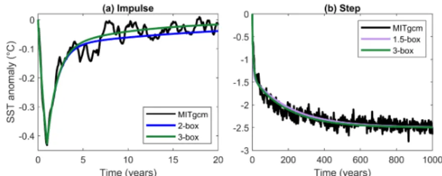
The first part of this thesis isolates the impact of the deep ocean in the surface response to volcanic cooling. Relaxation of the surface temperature follows a two-timescale decay, due to ocean heat exchange being significantly stronger than climatic feedbacks. Deep ocean cooling sequestration helps explain long periods of cold climate that occurred, for example, during the Little Ice Age.

The second part explores the volcanic forcing required to initiate state transitions in a GCM with multiple climate equilibria. Snowball transitions require cooling on the order of -100 𝑊 𝑚−2for several decades. These transition timescales are a consequence of the whole water column needing to be cooled to the freezing point before sea ice develops at the surface.

The third part investigates biogeochemical interactions between oceans and sea ice around Antarctica. During the glacial cycles of the Pleistocene, sea ice may have helped trap carbon in the ocean by inhibiting 𝐶𝑂2 outgassing. This work shows

that flux capping may be weakened by the effect of sea ice on reducing the light available for biological productivity. Consequently, a large sea ice fraction is required to effectively cap the flux of carbon to the atmosphere.

(4)

The final part of the thesis explores sea ice / ocean interactions at the eddy-scale. When sea ice is motionless relative to underlying mesoscale eddies, frictional drag at the surface generates patterns of Ekman pumping and suction, which mix the upper ocean. This mechanism brings warm waters up to the surface and can melt 10% of sea ice during winter and spring. Negative feedbacks ensure that sea ice is recovered in the following months, such that this mechanism does not accumulate sea ice melt over the years but changes its seasonality.

Thesis Supervisor: John Marshall

(5)

Acknowledgments

I would like to start by thanking my advisor John Marshall for guiding me through this thesis over the last five years. It was a privilege to learn from his experience, and I am very grateful for his patience, his support, his good humor, and for allowing me the flexibility to pursue a wide range of research interests. I have learnt a lot from his unique ability to turn difficult problems into much simpler ones, and I hope to carry these lessons for the rest of my career. I also wish to thank my thesis committee for their guidance and support throughout the process: Tim Cronin for teaching me most of what I know about radiation in the atmosphere and his help with Chapters 2 and 3, Mick Follows for teaching me about the carbon cycle and his guidance throughout Chapter 4, David Ferreira for his help with Chapter 3 and for inspiring the idea behind Chapter 4, and David McGee for his insightful comments on Chapters 2, 3 and 4, and for piquing my interest in paleoclimate early in my first year at MIT. I would also like to thank Raffaele Ferrari, Susan Solomon, Paul O’Gorman, Gianluca Meneghello, Ed Doddridge, Eduoardo Moreno-Chamarro, Hajoon Song, Maike Sonnenwald, Jonathan Lauderdale, Brian Green and Yavor Kostov for being so generous with their time and helping me tackle the various research questions posed in my thesis. Also, none of this work would have been possible without Jean-Michel Campin, who tirelessly answered all my questions about the MITgcm. I am also grateful for the Journal of Climate reviewers of Chapters 2 and 3, who helped improve these two manuscripts. Regarding funding, I acknowledge support from the John Carlson fellowship, the FESD Ozone project and the Houghton fund.

I would also like to thank my friends who helped create a positive and stimulating environment in the EAPS department, including Martin Wolf, Charles Gertler, Mar-garet Duffy, Rohini Shivamoggi, Megan Lickley, and many others. I am grateful for the wonderful staff in the department including Roberta Allard, Brandon Millardo, Jennifer Fentress, Darius Collazo and others, who make our lives so much easier on

(6)

the day to day. Outside the department, I want to thank my friends for their sup-port, their camaraderie and for the shared laughter during our years together in grad school. I am also overwhelmed by the variety and number of opportunities I was able to experience while at MIT, including the Arctic research cruise I participated in during my fourth year. I certainly feel very privileged to have taken part in them. Finally, and most importantly, I would like to thank my parents and brother for their hard work, love and support throughout the years.

(7)

List of Figures

2-1 Surface temperature response of the box model to an idealized Pinatubo eruption (-4 𝑊 𝑚−2 for a year) in the 1-box case (red) and 2-box cases (blue) in terms of the ratio of ocean mixing strength to the climatic feedback parameter 𝜇 = q/𝜆 with 𝜆 = 1.5 𝑊 𝑚−2𝐾−1. All other pa-rameters are as in Table 2.1. The ‘area under the curve’ is the same in all cases when integrating to infinity, but with a smaller peak and a longer ‘tail’ as q (or 𝜇) increases. . . 43

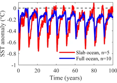
2-2 MITgcm responses (with monthly-mean data) to a Pinatubo-like forc-ing (-4 𝑊 𝑚−2 for a year) and a 10×Pinatubo forcing (-40 𝑊 𝑚−2 for a year) for the slab ocean in red and the full ocean configuration in blue. (a) Ensemble mean responses normalized with respect to their peak cooling temperature. (b) Non-normalized responses for the Pinatubo forcing with the shaded envelopes of 5 ensemble members for the slab ocean (red) and 10 ensemble members for the full ocean (blue). The solid lines are the corresponding ensemble mean. (c) Non-normalized responses for the 10×Pinatubo forcing with one ensemble member for the slab and full ocean respectively. . . 46

(14)

2-3 MITgcm zonally-averaged temperature anomaly in the ocean with depth and latitude in the full ocean configuration. The temperature evolu-tion is shown for 2, 5 and 10 years after the erupevolu-tion initiaevolu-tion in the left, middle and right panels respectively. The top panels are the mean responses of 10 ensemble members for the Pinatubo-like forcing (-4 𝑊 𝑚−2 for a year) and the bottom panels are the responses for a single ensemble member of the 10×Pinatubo forcing (-40 𝑊 𝑚−2 for a year). The thick black line represents the model-diagnosed zonally-averaged mixed layer depth. . . 47

2-4 MITgcm ensemble-mean response (with monthly-mean data) to a Pinatubo-like eruption (-4 𝑊 𝑚−2 for a year) every 10 years in the slab ocean (red) and full ocean (blue) configurations. The slab and full ocean configuration were run for 5 and 10 ensemble members respectively. . 48

2-5 2-box model comprising a mixed layer of depth ℎ1 and a deeper ocean

of depth ℎ2 with temperature anomalies 𝑇1 and 𝑇2 respectively. The

model is driven from the top by an external forcing F and damped by the climate feedback 𝜆𝑇1. The two boxes exchange heat through the

(15)

2-6 Temperature responses of the box model (solid lines) and the ensemble-mean MITgcm (dotted lines) to an idealized Pinatubo forcing (-4 𝑊 𝑚−2 for a year). (a) Fits to monthly-averaged MITgcm full ocean response (dotted blue) using the 2-box (solid blue) and the 1.5-box model (solid purple), and fit to the slab ocean MITgcm response (dotted red) using a 1-box model (red). (b) SST (dotted blue) and temperature at 120 m depth (dotted orange) from the MITgcm full ocean configuration with the corresponding 2-box model temperatures 𝑇1 (solid blue) and

𝑇2 (solid orange). The GCM temperature at 120 m depth and 𝑇2 are

multiplied by 5 for clarity. (c) Fits to the yearly-averaged MITgcm full ocean response (dotted blue) using the 2-box model and the 1.5 box model. . . 55

2-7 Fits to the MITgcm full ocean response. (a) Fits to the ensemble-mean idealized Pinatubo response (-4 𝑊 𝑚−2 for a year) over monthly-averaged data (black) using a 2-box (blue) and a 3-box (green) model. (b) Fits to the MITgcm step response with -4 𝑊 𝑚−2 forcing (black) using the 1.5-box (purple) and 3-box models. . . 56

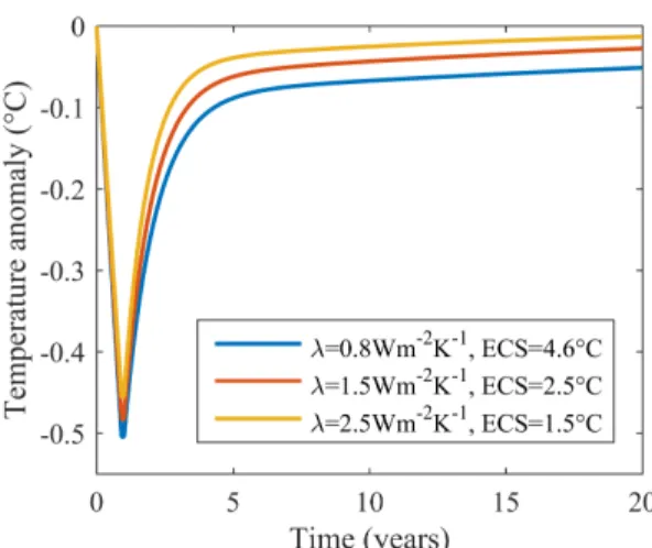
2-8 2-box model responses to an idealized Pinatubo forcing (-4 𝑊 𝑚−2 for a year) for a range of 𝜆 (or ECS) values. All other parameters are fixed to those in Table 2.1. . . 58

2-9 Normalized temperature envelope 𝑇𝑒𝑛 for a series of uniform and

reg-ularly spaced eruptions in the 2-box model. Each dot represents the peak cooling temperature after a new eruption. Parameter sensitivity is explored for (a) the climate sensitivity 𝜆, (b) the mixed layer depth ℎ1, (c) the ocean exchange parameter q and (d) the time interval

be-tween eruptions 𝜏 All fixed parameters are as in Table 2.1 and the default 𝜏 value is 10 years. . . 63

(16)

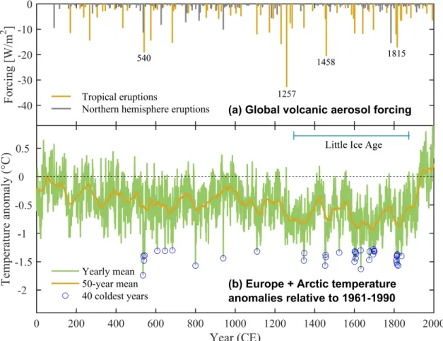
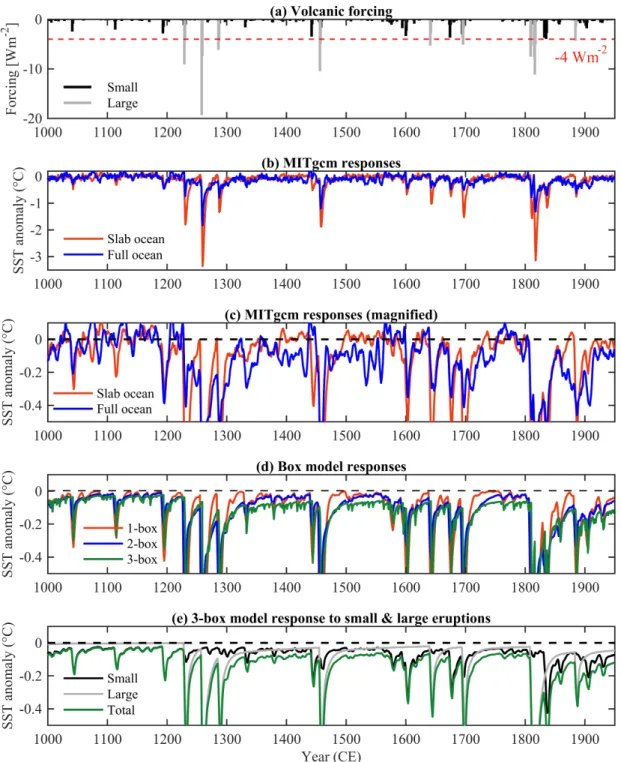
2-10 (data from Sigl et al. (2015)): (a) 2000-year reconstruction of global volcanic aerosol forcing from sulfate composite records from tropical (orange) and Northern Hemisphere (gray) eruptions. (b) 2000-year record of reconstructed summer temperature anomalies for Europe and the Arctic relative to 1961-1990 shown at yearly resolution (green) and as a 50-year running mean (orange). The 40 coldest single years are indicated with blue circles and the approximate duration of the Little Ice Age is shown. . . 65

2-11 (a) Tropical volcanic forcing of the last millennium (A. LeGrande, NASA GISS, personal communication) divided into small (> -4 𝑊 𝑚−2) and large eruptions (≤ -4 𝑊 𝑚−2). (b) responses of the MITgcm cou-pled model with a full ocean (blue) and a slab ocean (red) to the volcanic forcing shown in (a). (c) 5-year running mean of (b) on a magnified scale. (d) 1-box (red), 2-box (blue) and 3-box model (green) responses to the forcing. (e) 5-year running mean of the 3-box model response to the small (black), large (gray) and total (green) volcanic forcing. . . 68

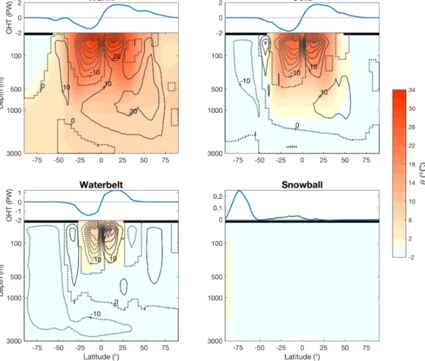
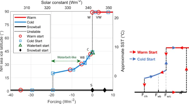
3-1 A graphical representation of the 3 equilibria of our climate model: Warm, Cold and Snowball. On the x-axis, we plot the latitude of NH sea ice extent (bottom axis) and ice fraction (top axis). On the y-axis, we plot the ocean-mean potential temperature, 𝜃, (left axis) and energy level (right axis). The thermal energy stored in the ocean dominates over all other sources. The unstable (dotted) lines are linear interpolations between the stable states found in the model. In these ranges of sea ice latitudes and 𝜃, no stable solution can be found. The globes show the SST and sea ice extent of the Warm reference, Cold reference, Waterbelt and Snowball states (from right to left). . . 76

(17)

3-2 Zonally-averaged ocean potential temperature (color shading) for the Warm reference, Cold reference, Waterbelt and Snowball states ex-pressed on a stretched depth scale to highlight the thermal structure of the upper ocean. The annual-mean sea ice cover in each hemi-sphere is denoted by the thick black lines. The zonally-averaged ocean overturning streamfunction (in Sv) is shown with clockwise circulation represented by solid lines and anticlockwise circulation by dotted lines, with a contour interval of 10 Sv. The zonally-averaged meridional ocean heat transport (in PW) is shown above each panel. Note the different scales of OHT. . . 79

3-3 (left) Bifurcation diagram of the climate model expressed in terms of the NH sea ice latitude (left axis) versus the forcing F (bottom axis). F is calculated relative to the reference solar constant 𝑆0 = 341.5 𝑊 𝑚−2.

The right axis indicates the approximate global mean SST and the top axis shows the solar constant. The thick lines show the range of stable Warm (red), Cold (blue) and Snowball (black) states. The black dotted lines indicate unstable NH sea ice latitudes. Each red circle, blue square, green triangle and black diamond shows the equilibrated state of a simulation started from the Warm (W), Cold (C), Waterbelt (WB) and Snowball (S) states, respectively. (right) Schematic plot (not to scale) of the hysteresis loop. Stable and unstable branches are represented by solid and dotted lines, respectively. The red arrows describe a path that starts from a Warm state, cools to a Snowball and exhibits hysteresis while warming back up. The blue arrows indicate a path that starts from a Cold state and heats up to the Warm branch without hysteresis. 𝐹𝑤/𝑐 and 𝐹𝑐/𝑠are transition thresholds between the

Warm/Cold and the Cold/Snowball equilibria respectively. 𝐹𝑤𝑏 (= -5

𝑊 𝑚−2) is the forcing below which the Cold states become Waterbelt-like. . . 80

(18)

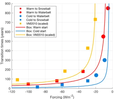
3-4 Transition times to reach either the Waterbelt (circles) or Snowball (squares) climate for step simulations starting from the Warm reference state (red) and Cold reference state (blue). The Snowball transition times obtained by VM2010 are also plotted (in orange squares) and scaled by a factor 𝑓𝑣𝑚 = 1.5 for ease of comparison with simulations

starting from the Warm reference state. Solid lines are corresponding estimates from the 1-box model with the following parameter values: for a Warm start, 𝜆𝑤 = 0.72 𝑊 𝑚−2 and H = 2416 m (red line); for a

Cold start, 𝜆𝑐= 0.95 𝑊 𝑚−2 and H = 1149 m (blue line); for VM2010,

𝜆𝑣𝑚 = 3.3 𝑊 𝑚−2, H = 2603 m and 𝑓𝑣𝑚 = 1.5 (orange line). . . 84

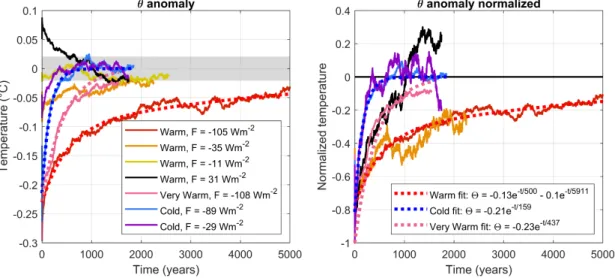
3-5 Time evolution of the whole-ocean mean potential temperature anomaly following 1-year long eruptions in our coupled model for a range of forcing magnitudes and starting states. (left) Absolute temperature anomaly response, where the shading represents the 2𝜎 range of un-forced variability in the control run. (right) Normalized responses with respect to the peak cooling, which in each case occurs at the end of the first year, the time at which the forcing is turned off. Solid lines are simulation results from the climate model, whereas dotted lines are exponential fits to the following simulations: F = -105 𝑊 𝑚−2 run from Warm (red), F = -89 𝑊 𝑚−2 from Cold (blue) and F = -108 𝑊 𝑚−2 from Very Warm (pink). . . 88

(19)

3-6 Global-mean ocean potential temperature anomaly, plotted as a func-tion of depth, following impulse cooling forcings lasting 1 year, with a 50-year time averaging window. The shading represents the 2𝜎 level of unforced variability estimated from the relevant control simulation. The panels present results from the following simulations: (a) F = -105 𝑊 𝑚−2 starting from Warm, (b) F = -35 𝑊 𝑚−2 starting from Warm, (c) F = +31 𝑊 𝑚−2 starting from Warm, and (d) F = -108 𝑊 𝑚−2 starting from Very Warm. The dotted lines in panel (a) show temper-ature profiles obtained from a 1D diffusive model with a diffusivity 𝜅 = 3 × 10−5 𝑚2_𝑠−1_{. . . .} ₉₁

3-7 (left) The response of global-mean ocean temperature, 𝜃, to repeated 1-year eruptions every 𝜏𝑖 = 10 years beginning from a Warm start with

F = -105 𝑊 𝑚−2 (red) and a Cold start with F = -89 𝑊 𝑚−2 (dark blue). Step simulation responses are also shown for a Warm start with F = -11 𝑊 𝑚−2 (orange) and for a Cold start with F = -9 𝑊 𝑚−2 (light blue). Box model step responses for a Warm start with F = -11 𝑊 𝑚−2 (black dotted) and for a Cold start with F = -9 𝑊 𝑚−2 (green dotted). (right) Sea ice fraction response in the climate model simulations. . . 93

(20)

3-8 Estimates of state transition times for forcings consisting of repeated volcanic eruptions lasting 1 year, every 𝜏𝑖 years. The transition times

are estimated using the step response under an average forcing 𝐹𝑎𝑣,

for a range of forcing magnitudes F and eruption intervals 𝜏𝑖. The

points below the white dotted line are transitions to a Snowball. Points between the white and red dotted lines are transitions to the Waterbelt climate. Points between the red and black dotted lines are transitions to Cold. The straight contours represent constant values of 𝐹𝑎𝑣. Panel

(a) and (b) show transition times when starting from the Cold and Warm reference climates, respectively. Note the different scales for the two panels. . . 95

4-1 Simplified schematic representing the 2-cell residual overturning circu-lation in the Southern Ocean. The thick black lines show these two cells flowing from the deep ocean up to the surface, travelling within the mixed layer (in red), and then re-subducting into the deep ocean. The top cell returns northward as intermediate waters whereas the bot-tom cell sinks near the shelf to form botbot-tom waters. This overturning circulation carries carbon and nutrient-rich waters up to the surface, which drives carbon outgassing in the South and carbon uptake in the North, as represented with the thin vertical arrows. Sea ice (in blue) can affect both these processes by capping the air-sea flux and reducing light availability. . . 101

(21)

4-2 Equilibrium solution in the 2D channel model. (top) The residual streamfunction is shown in the filled contours, where positive is clock-wise and negative is anti-clockclock-wise. The black contours are isopycnals referenced at the surface. The red arrows indicate the direction of the surface flow, which reverses around 65∘S; (bottom) the filled contours show the 𝐷𝐼𝐶 concentration in the model and the orange contours indicate potential temperature. The horizontal bars show the summer (dark gray) and winter (light gray) sea ice edges. . . 107

4-3 Seasonal climatology of air-sea carbon fluxes and sea ice fractions from zonal-mean observations and the channel model simulation. The ob-served fluxes (dashed lines) are taken from Landschützer et al. (2017) in the period 1998 to 2011, and error bars indicate one standard deviation temporal variability. The observed sea ice fractions are obtained from Cavalieri et al. (1996) and averaged between 1978 and 2018. Channel model fluxes are taken from simulations with 𝑝𝐶𝑂𝑎

2 = 278 ppm (solid

lines) and 370 ppm (dotted lines). The individual panels show (a) an-nual mean, (b) summer (DJF), (c) fall (MAM), (d) winter (JJA) and (e) spring (SON) conditions. Outgassing is defined as positive. . . . 109

(22)

4-4 Decomposition of the annual mean air-sea carbon flux in the channel model using the method of LAU16 (positive is outgassing). The thin black line is the model-diagnosed flux and the thick black line is the to-tal reconstructed flux 𝐹𝐶𝑂2. The red line shows the heat-driven carbon

saturation flux 𝐹ℎ𝑒𝑎𝑡. The orange line is the fresh water-driven carbon

flux 𝐹𝑓 𝑟𝑒𝑠ℎ, which includes the effects of direct dilution of 𝐷𝐼𝐶, salt

and alkalinity. The dotted blue line is the biological flux 𝐹𝑏𝑖𝑜, which

includes the soft tissue and carbonate pumps. The blue dashed line is the disequilibrium flux component 𝐹𝑑𝑖𝑠, and the solid blue line is the

sum 𝐹𝑏𝑖𝑜 + 𝐹𝑑𝑖𝑠. All the colored solid lines add up to the reconstructed

flux (thick black line). The horizontal bars show the summer (dark gray) and winter (light gray) sea ice edges. The background state has 𝑝𝐶𝑂𝑎₂ = 278 ppm. . . 113

4-5 Air-sea carbon flux in the channel model for cases where the seasonal ice cover affects capping only (orange), light attenuation only (green), or both together (solid black). The ‘no ice’ case is also shown in the dotted black line. The horizontal bars indicate the model’s sea ice fraction with latitude over the seasons, as well as the PAR undisturbed by ice. . . 114

4-6 Air-sea carbon flux integrated over (a) the imposed ice zone and (b) the whole domain for three sets of experiments where ice affects: cap-ping only (orange), light attenuation only (green), and both together (black). The imposed sea ice is uniform and constant throughout the year between 70∘S and 55∘S. The scatters show channel model results and the solid lines are corresponding fits from the analytical model. The background state has 𝑝𝐶𝑂𝑎₂ = 278 ppm. . . 116

(23)

4-7 Meridional structure of the air-sea carbon flux in the channel model (left) and the analytical model (right) for a range of sea ice fractions. Each row shows experiments in which sea ice affects capping only (top), light attenuation only (middle), and both together (bottom). Out-gassing is defined as positive. The extent of the uniform and time-invariant sea ice is highlighted in blue. The black arrows show the flow direction in the imposed ice zone, and the black dots indicate the lo-cation of either the upwelling point (in the channel model) or the inlet (in the analytical model). The background state has 𝑝𝐶𝑂₂𝑎 = 278 ppm. 118

4-8 As in Figure 4-6 but in the background state where 𝑝𝐶𝑂₂𝑎 = 370 ppm. 119

4-9 Air-sea carbon fluxes integrated over the imposed ice zone and normal-ized with respect to the integrated flux when no ice is present. Black scatters show the channel model results in the reference case where sea ice extends between 70∘S and 55∘S. Blue scatters are channel model results obtained by halving the length of the imposed ice zone (70∘S and 63∘S) and integrating over that reduced domain. Solid lines are corresponding results from the analytical model using the full ice zone length L (in black) and half its length 𝐿/2 (in blue). In these sim-ulations, sea ice affects both capping and light attenuation together (𝛼𝑒= 𝛼𝑏 = 𝛼). The background state has 𝑝𝐶𝑂𝑎2 = 278 ppm. . . 121

4-10 As in Figure 4-6, except that the imposed sea ice is only applied during the winter and spring months (June to November). The rest of the year is completely ice-free. . . 122

(24)

4-11 Annual mean air-sea carbon flux in the simulations with no imposed ice (solid black line), in a simulation with 75% uniform ice cover (solid green line) and in a simulation with intermittent ice cover averaging 75% (dashed green line). The ice extends between 70∘S and 55∘S, and affects capping only. The net integrated flux over the ice zone is 19 ·106_𝑔𝐶𝑚−1_𝑦𝑟−1 _{for the no ice case, 8.6 ·10}6_𝑔𝐶𝑚−1_𝑦𝑟−1 _{for the}

uniform ice cover case, and 7.6 ·106𝑔𝐶𝑚−1𝑦𝑟−1 when ice is applied intermittently. Outgassing is defined as positive. . . 123

4-12 𝐷𝐼𝐶 anomaly after 100 years in simulations where the sea ice fraction is 100% between 70∘S and 55∘S, and applied year-round. Ice affects (a) capping only, (b) light attenuation only, and (c) both together. The anomaly is calculated relative to a simulation with no imposed sea ice. The background state has 𝑝𝐶𝑂𝑎

2 = 278 ppm. . . 125

5-1 Schematic of the ‘Eddy-Ice-Pumping’ mechanism (EIP) in the South-ern hemisphere. When sea ice is stationary relative to the ocean, the ice-ocean stress 𝜏𝑖 opposes the eddy motion 𝑢, driving Ekman suction

in anticyclones and Ekman pumping in cyclones. Upwelling of warm waters may melt sea ice in anticyclones, whereas downwelling in cy-clones may shield sea ice away from warm waters, potentially allowing for thicker ice growth. . . 132

(25)

5-2 Annual and zonal mean state of the channel model at equilibrium. (Top) Potential temperature (filled contours), potential density 𝜎0(grey

line contours in the top 210 m) and 𝜎2 (grey contours between 210

-4000 m). The annual mean sea ice fraction is shown in the blue con-tours at the top of the panel. The colored lines show the summer (red) and winter (green) MLD, both based on a ∆𝜎0 = 0.06 𝑘𝑔𝑚−3 criterion.

(Bottom) Salt (filled contours) and residual streamfunction in Sv [ = 106_𝑚3_𝑠−1_{] (grey line contours; filled clockwise, and dashed}

anticlock-wise). The solid bars at the top of the panel indicate the minimum (dark gray) and maximum (light gray) sea ice extent. . . 134

5-3 Snapshots of (a) sea ice fraction, (b) normalized surface vorticity 𝜁/f (c) Ekman vertical velocity 𝑤𝑒𝑘, (d) subsurface vertical velocity 𝑤𝑠, (e)

normalized surface vorticity minus sea ice vorticity (𝜁 - 𝜁𝑖)/f, and (f)

eddying power transfer between ice and ocean 𝑃_𝑖′ taken in September, and shown over a subset of the model domain. The green dashed lines show the limits of the continental slope and the shelf, and the dotted black line shows the zonal mean sea ice edge. . . 136

5-4 (a-b) Snapshots of (a) the zonal and (b) the meridional stresses on the ocean surface in September. The colored contours show the net surface stresses in the simulation where the ice stress is ‘on’. The line plots show zonal mean stresses for the simulations where the ice stress is ‘on’ (blue) and ‘off’ (red). (c-d) September snapshots of subsurface vertical velocity 𝑤𝑠 within the ice zone for the cases where the ice stress is (c)

‘on’ and (d) ‘off’. The green dashed lines indicate the edges of the continental slope and shelf respectively. The black dotted line shows the zonal mean sea ice edge. . . 138

(26)

5-5 Open ocean composites taken between y = 1900 - 2900 km in the channel model for cyclones (panels (a) to (f)) and anticyclones (panels (g) to (l)). The composites are projected on to a characteristic eddy radius ˆ𝑟 = 60 km and the horizontal coordinates ˆ𝑥 and ˆ𝑦 span -2ˆ𝑟 to +2ˆ𝑟. The filled contours in panels (a) to (d) show vertical cross-sections through the center of the composite in the x-direction for 𝜃, S, 𝜎0 and

the vertical velocity 𝑤, respectively. The white lines in panels (a) to (c) indicate the MLD. Panel (d) also shows 𝑤𝑠 (in black) and 𝑤𝑒𝑘 (in red).

The filled contours in panels (e) and (f) show plan views of the MLD and 𝑤𝑠, respectively. The yellow line in panel (e) is a characteristic sea

surface height contour. Panels (g) to (l) show corresponding results for the anticyclone composite. . . 140

5-6 Compact ice zone composites with ice stress ‘on’ taken between y = 400 - 800 km in the channel model for cyclones (panels (a) to (f)) and anticyclones (panels (g) to (l)). The composites are projected on to a characteristic eddy radius ˆ𝑟 = 30 km and the horizontal coordinates ˆ

𝑥 and ˆ𝑦 span -2ˆ𝑟 to +2ˆ𝑟. The filled contours in panels (a) to (d) show vertical cross-sections through the center of the composite in the x-direction for 𝜃, S, 𝜎0 and the vertical velocity 𝑤, respectively. The

white lines in panels (a) to (c) indicate the MLD. Panel (d) also shows 𝑤𝑠 (in black) and 𝑤𝑒𝑘 (in red). The filled contours in panels (e) and

(f) show plan views of the MLD and the area-weighted average sea ice thickness, respectively. The yellow line in panel (e) is a characteristic sea surface height contour. The black line in panel (f) is the net heat flux to the ice. Panels (g) to (l) show corresponding results for the anticyclone composite. . . 143

(27)

5-7 Compact ice zone composites with ice stress ‘off’ taken between y = 400 - 800 km in the channel model for cyclones (panels (a) to (f)) and anticyclones (panels (g) to (l)). The composites are projected on to a characteristic eddy radius ˆ𝑟 = 30 km and the horizontal coordinates ˆ

𝑥 and ˆ𝑦 span -2ˆ𝑟 to +2ˆ𝑟. The filled contours in panels (a) to (d) show vertical cross-sections through the center of the composite in the x-direction for 𝜃, S, 𝜎0 and the vertical velocity 𝑤, respectively. The

white lines in panels (a) to (c) indicate the MLD. Panel (d) also shows 𝑤𝑠 (in black) and 𝑤𝑒𝑘 (in red). The filled contours in panels (e) and

(f) show plan views of the MLD and the area-weighted average sea ice thickness, respectively. The yellow line in panel (e) is a characteristic sea surface height contour. The black line in panel (f) is the net heat flux to the ice. Panels (g) to (l) show corresponding results for the anticyclone composite. . . 145

5-8 Seasonal evolution of the area-weighted average sea ice thickness (top) and heat fluxes (bottom) within the compact ice zone (y = 400 - 800 km) calculated for the first year of the sensitivity simulation; (left) ice stress ‘on’, and (right) ice stress ‘on’ minus ‘off’. . . 147

5-9 Vertical profiles of (a) 𝜃, (b) 𝑆, (c) 𝑁2_{and (d) 𝐸𝐾𝐸 within the seasonal}

ice zone (y = 400 - 800 km, zonal mean) calculated for the first year of the sensitivity simulation and averaged over seasons: summer in red (JF), fall in green (MAM), winter in blue (JJA), and spring in orange (SON). The left panel of each subplot shows ice stress ‘on’ and the right panel shows ‘on’ minus ‘off’. . . 148

(28)

5-10 4-year evolution of the ice stress ‘on’ minus ‘off’ simulations for (a) 𝜃, (b) 𝑆, (c) area-weighted average sea ice thickness, (d) net heat flux from the atmosphere to the ocean, and (d) net heat flux to sea ice. The vertical dotted lines separate each individual year. . . 149

A-1 Linear albedo gradient imposed at the surface of the MITgcm model. The grid is in a cubed sphere configuration with 32× 32 points per face, with a nominal horizontal resolution of 2.8∘ . The thick black lines indicate the solid ridges of the ‘double-drake’ setup extending from the North Pole to 35∘ S and set 90∘ apart. . . 160

B-1 Bifurcation diagrams obtained from the EBM for a range of 𝛿 values. All other parameters are fixed to: A = 210 𝑊 𝑚−2, B = 1.5 𝑊 𝑚−2𝐾−1, 𝑎0 = 0.7, 𝑎𝑖 = 0.4, 𝑠2 = -0.48, ℎ𝑚𝑖𝑛 = 0.67m, 𝑘𝑖 = 2 𝑊 𝑚−2𝐾−1, 𝑇𝑓 = 0 ∘

C, Ψ = 4 PW and N = 4. Solid curves are obtained from the analytical model, whereas the dotted lines are results from the numerical solution of the EBM, which only picks out the stable branches of the diagram. 163

D-1 Composite means of anticyclones for 𝑤𝑠 (left) and 𝑤𝑠𝑡𝑒𝑟𝑛 (right). The

composites are taken in the open ocean (top), in the compact ice zone with ice stress ‘on’ (middle) and in the compact ice zone with the ice stress ‘off’ (bottom). . . 168

(29)

List of Tables

2.1 2-box model parameters obtained by curve-fitting the monthly SST response of the full ocean MITgcm to an idealized Pinatubo eruption. 54

(30)

(31)

Chapter 1 Introduction

1.1 Volcanic eruptions and the climate

1.1.1 Equilibrium versus transient climate sensitivity

The thermal heat capacity of the global oceans is by far the largest of all other components of the climate system. This property affords the ocean a fundamental role in the transient response of the climate to any changes in its energetic balance. When the Earth is subjected to a radiative forcing, the time taken for the system to reach its new equilibrium depends on how effectively temperature anomalies are transferred to the deepest layers of the ocean. Below the ocean’s mixed layer (∼ 50 -100 m), this process is not particularly efficient, and may take between several decades to thousands of years. While the surface of the Earth may reach a quasi-equilibrated state much faster than the rest of the ocean (years to decades), its characteristic response timescales still depend on the amount of heat absorbed by the deeper ocean.

(32)

Volcanic eruptions are an impulse-like forcing to the climate. The response of the system is thus a natural ‘Green’s function’ that can teach us fundamental properties regarding climate sensitivity. Large volcanic events are often followed by surface cool-ing, caused by the ejection of shortwave-scattering aerosols into the stratosphere for one or two years (Robock (2000)). The recovery of the sea surface temperature (SST) following this impulse-like forcing may last well beyond the end of the eruption, owing to the ocean’s large heat capacity. This thesis studies these characteristic relaxation timescales in an attempt to parse the relative importance of surface damping versus oceanic heat uptake in the response, and thus the ratio between equilibrium and tran-sient climate sensitivity. Contrasting impulse versus step responses then allows us to connect with studies investigating climate scenarios under increased greenhouse gas concentrations in the context of global warming (Gregory (2010), Held et al. (2010), Geoffroy et al. (2013b), Merlis et al. (2014)) .

1.1.2 Oceanic prolongation of the volcanic response

Following a volcanic eruption, the sequestration of cold temperature anomalies by the ocean can shield them away from damping processes acting at the surface. The cooling anomaly then returns to the surface over longer timescales, over which the effects of multiple eruptions can accumulate. This long term memory of the ocean may have important consequences for paleoclimate. A number of recent studies have emphasized the role of volcanoes in triggering and maintaining the Little Ice Age (∼ 1250-1850), beyond the effects of reduced insolation and land use changes (Free and Robock (1999), Crowley et al. (2008), Stenchikov et al. (2009)). The prolongation of the volcanic response by the presence of the deeper ocean may help explain the discrepancy between the short-lived nature of each eruption and the observed decades to centuries of cooling during that time. The recent discovery of cold temperature anomalies originating from the Little Age in the deep ocean lend some observational support to this argument (Gebbie and Huybers (2019)). This thesis addresses whether

(33)

small or large eruptions matter the most for producing a long lasting response, and investigates the contribution of decadal versus centennial scale accumulation of the response.

1.1.3 Snowball Earth initiation

The paleoclimate record suggests that certain volcanic eruptions in the distant past may have been several times more powerful than the ones experienced during the Holocene. For instance, the Toba eruption that occurred approximately 75 ka may have produced a radiative forcing on the order of -100 𝑊 𝑚−2, compared to -4 𝑊 𝑚−2 for the Mount Pinatubo eruption in 1991 (Jones et al. (2016)). Macdonald and Wordsworth (2017) suggest that a succession of such eruptions may have been power-ful enough to plunge the Earth into a Snowball state. These authors present evidence of a sulfur-rich evaporite basin, whose onset coincided with the start of the Sturtian Snowball event (∼ 750 Ma ago), and which could have provided the sulfur required for volcanic cooling. This thesis explores the forcing required for such a state transition to occur, as well as the dependence on the starting state. The transition timescales depend on the deep ocean’s heat capacity, since intense surface cooling causes convec-tive events that can mix the entire ocean column. Forcing thresholds are investigated in light of a bifurcation diagram, whose stable states and hysterisis properties are set by a balance between meridional heat transport and the ice-albedo feedback.

1.2 The role of sea ice on the global carbon cycle

The long timescales associated with the deep ocean circulation affect not only temper-ature, but also the distribution of tracers such as dissolved inorganic carbon (𝐷𝐼𝐶). The ocean stores more than 50 times the amount of carbon as the atmosphere, and

(34)

hence can act as a buffer to changes in the atmospheric carbon concentration (𝑝𝐶𝑂₂𝑎). Proxy data from the Pleistocene (2.5 Ma to 11.7 ka) suggest that glacial times were characterised by a low 𝑝𝐶𝑂₂𝑎 of around 190 ppm, compared to interglacial values around 270 ppm. Many studies have associated this glacial decrease in 𝑝𝐶𝑂𝑎

2 to

en-hanced deep ocean carbon storage initiated at high latitudes (e.g. Toggweiler and Sarmiento (1985a), Sigman and Boyle (2000), Stephens and Keeling (2000), Ferrari et al. (2014)). The increase in the ocean’s solubility under a colder climate only explains a fraction of this 𝐶𝑂2 drawdown. Hence, a variety of other mechanisms

have have been invoked, including changes in oceanic circulation, enhanced biological carbon pump and reduced air-sea exchanges due to sea ice expansion. Currently, state-of-the-art GCMs cannot consistently reproduce the observed decrease in 𝑝𝐶𝑂₂𝑎 during glacial periods (Otto-Bliesner et al. (2006), Braconnot et al. (2007)), mostly due to a poor representation of high latitude processes in both the modern and glacial states. This motivates the need for a better understanding of polar regions in terms of their physics and their biogeochemistry.

The Southern Ocean represents a significant source of uncertainty in today’s global carbon cycle. The difficulty of access makes it a relatively poorly sampled basin, particularly during the winter and spring months due to an extended sea ice cover. Around Antarctica, the ocean’s meridional overturning circulation brings DIC- and nutrient-rich waters from the deep ocean up to the surface, where carbon may escape to the atmopshere (outgassing). However, DIC may also be utilized by phytoplankton to form organic particles that ultimately sink into the deep ocean (uptake). The balance between these two processes plays an outsized role in setting the global 𝑝𝐶𝑂𝑎

2,

particularly over glacial/interglacial timescales. Furthermore, over a seasonal cycle, the growth and retreat of the sea ice pack can affect physical and biological processes occuring in the region. Sea ice can act as a lid that reduces air-sea carbon exchanges (capping), but it may also attenuate the amount of light available for organisms living in the ocean, and thus reduce the formation of sinking organic particles. This thesis introduces a novel framework to study the balance between these mechanisms,

(35)

expressed in terms of a residence, an exchange and a biological timescale. We find that when these three timescales are of the same order of magnitude, as they are in the modern climate, the light attenuation effect of sea ice can strongly compensate its flux capping tendency. This compensation may thus have important consequences for interpreting the influence of sea ice on the global carbon cycle.

1.3 Eddy-scale sea ice/ocean interactions

Sea ice clearly plays an important role in the global climate system. Over the last few decades, the declining sea ice coverage in the Northern hemisphere and its role in Arctic amplification have already altered the local climate, through increased surface air temperatures, Greenland ice sheet melt and river warming (Pithan and Mauritsen (2014)). Future changes in sea ice coverage and seasonality may also have a global impact through their influence on deep and bottom water formation in the Arctic (Mauritzen and Häkkinen (1997)) and the Antarctic (Ohshima et al. (2016)), re-spectively. The importance of sea ice for both modern and past climates motivates a better understanding of its interactions with the surrounding atmosphere and oceans. GCMs are currently not able to reproduce the observed trends or spatial patterns in Antarctic sea ice over the last decades (Turner et al. (2013)). In the Arctic, the rapid decline of sea ice and the widening of the marginal ice zone (MIZ) make it particularly challenging to predict future trends.

Past studies have highlighted the importance of oceanic eddies in bringing warm waters in contact with sea ice and in controlling its thickness distribution through basal melt, both in the Arctic and the Antarctic (Johannessen et al. (1987), Niebauer and Smith Jr. (1989), Smith and Bird (1991)). Global climate models are too coarse to faithfully reproduce the fine scale processes responsible for these vertical heat fluxes underneath sea ice. Moreover, the lack of instrumentation in the sea ice zone

(36)

means that many of these processes are currently not well observed and understood. This thesis describes a novel mechanism by which frictional ice / ocean interactions may drive large vertical heat fluxes in regions of compact sea ice, through Ekman pumping and suction. These enhanced vertical velocities are somewhat analogous to the ones generated by eddy-wind interactions in the open ocean, but underneath sea ice, the thermodynamic influence of the melt/freeze cycle can strongly modulate the response of eddies. We find that this mechanism can melt a significant amount of ice in winter and spring, and thereby change its seasonal cycle. Our model also predicts that the melting and freezing properties of sea ice impact the vertical structure of underlying eddies in ways that may soon be observable with the development of sensing technologies under ice.

1.4 Thesis overview

This thesis uses an array of climate models to study the various questions intro-duced above. Where possible, connections are drawn between model results, modern observations and the paleoclimate record. The thesis is organized as follows:

Chapter 2 uses an aquaplanet model with both slab and full ocean configurations to isolate the role of the deep ocean in the climate’s response to idealized volcanic eruptions. The study explores how the shape of the globally-averaged SST response changes due to heat exchanges with the deep ocean, and how this affects estimates of transient and equilibrium climate sensitivity. Results are interpreted with a hierarchy of box models that highlight the significance of the long relaxation timescales. The accumulation of a climate response following a succession of volcanic eruptions is then illustrated in the context of the Little Ice Age. The models show that when aided by ocean heat sequestration, clusters of large eruptions can have a cooling effect that lasts multiple decades. This chapter is largely based on the material published in

(37)

Gupta and Marshall (2018).

Chapter 3 explores accumulation of volcanic cooling as a possible trigger for Snowball Earth. This work uses a GCM with coupled ocean, atmosphere, land and sea ice dynamics, which supports three equilibrium states, namely Warm, Cold and Snowball. The GCM’s bifurcation diagram is generated by means of step-like forcings starting from each of the equilibrium states, and interpreted in light of an energy balance model (EBM). Transition timescales are investigated for step forcings, single eruptions and a succession of eruptions. These system’s characteristic transition timescales are then connected to the relevant ocean heat capacity for each of the starting states. Snowball transitions starting from the Cold state are found to be significantly more favorable than from the Warm state, but they still require a much more intense volcanic cooling than that predicted by Macdonald and Wordsworth (2017). This chapter is largely based on the material published in Gupta et al. (2019).

Chapter 4 makes use of a 2D channel model of the Southern Ocean to investigate the compensation between the capping and light attenuation effects of sea ice on surface carbon fluxes. The model is forced by realistic boundary conditions and produces an equilibrium state that matches reasonably well with observations. A decomposition of the air-sea carbon flux shows that in the annual mean, it is dominated by the balance between the upwelling of carbon-rich waters and uptake from biological ac-tivity. Numerical experiments are conducted with fixed physical dynamics and 𝑝𝐶𝑂𝑎

2,

while varying the amount of sea ice seen by the biogeochemistry package. A theory for the compensation between capping and light attenuation is developed from a 1D analytical model and tested with various sensitivity experiments in the channel. The compensation mechanism is found to be particularly significant for a large sea ice cover and during the months of spring. The material in this chapter is based on Gupta et al. (prep), as submitted to Global Biogeochemical Cycles.

(38)

3D channel model of the Southern Ocean. The seasonal ice zone in the model is realistically characterized by a temperature inversion whereby a cold and fresh layer of water protects sea ice from warmer waters at depth. In the compact ice zone, when eddies experience a drag from the overlaying sea ice, the resulting vertical Ekman velocities create temperature hotspots at the surface, which can melt sea ice. This mechanism is investigated via an eddy composite analysis performed separately over cyclones and anticyclones. The analysis reveals that the effectiveness of the melt mechanism is linked to the asymmetric way in which cyclones and anticyclones respond to the surface stress. The implications of this dynamic coupling between the ice and the ocean is discussed in light of sea ice thickness, vertical profiles, and their seasonality.

Chapter 6 reflects on the main conclusions of this thesis and suggests potential exten-sions for future research. The aim of this study was to develop a better understanding of processes linking the climate, the global ocean and sea ice. We used numerical cli-mate models in conjunction with idealized theory to formulate the essence of these mechanisms and test their range of applicability. Going forward, exploring some of these processes in more complex climate models and in observations could be a valu-able endeavour. Regarding the volcanic cooling work in Chapter 2, further studies could include a more thorough examination of the physical mechanisms responsible for sequestering cooling anomalies of the ocean, and a comparison with observational data from the Mount Pinatubo eruption. The multiple equilibria discussed in Chap-ter 3 could be investigated in more realistic climate models, and in particular the behavior of clouds under different climatic states should be explored further. Re-garding the effect of sea ice on the carbon cycle, a better understanding of biological activity underneath sea ice would be useful to substantiate the conclusions of Chapter 4. Finally, evidence of the ice / ocean interactions described in Chapter 5 could be explored in observational datasets underneath compact sea ice in the Arctic and the Antarctic. Some of the idea explored in Chapter 5 may also be extended to looser regions of sea ice, and potentially help us understand how polar regions will respond

(39)

(40)

(41)

Chapter 2 The climate response to multiple

volcanic eruptions mediated by ocean

heat uptake

Abstract

A hierarchy of models is used to explore the role of the ocean in mediating the response of the climate to a single volcanic eruption and to a series of eruptions by drawing cold temperature anomalies in to its interior, as measured by the ocean heat exchange parameter q [𝑊 𝑚−2𝐾−1]. The response to a single (Pinatubo-like) eruption comprises two primary timescales, one fast (year) and one slow (decadal). Over the fast timescale, the ocean sequesters cooling anomalies induced by the eruption into its depth, enhancing the damping rate of sea surface temperature (SST) relative to that which would be expected if the atmosphere acted alone. This compromises the ability to constrain atmospheric feedback rates measured by 𝜆 [ 1 𝑊 𝑚−2𝐾−1] from study of the relaxation of SST back toward equilibrium, but yields information about

(42)

the transient climate sensitivity proportional to 𝜆 + q. Our study suggests that q can significantly exceed 𝜆 in the immediate aftermath of an eruption. Shielded from damping to the atmosphere, the effect of the volcanic eruption persists on longer decadal timescales. We contrast the response to an ‘impulse’ from that of a ‘step’ in which the forcing is kept constant in time. Finally, we assess the ‘accumulation potential’ of a succession of volcanic eruptions over time, a process that may in part explain the prolongation of cold surface temperatures experienced during, for example, the Little Ice Age.

2.1 Introduction

Large volcanic eruptions are a natural, impulse-like perturbation to the climate sys-tem. The sulfur particles ejected into the stratosphere during these eruptions are rapidly converted to sulfate aerosols that diminish the net incoming solar flux at the top of the atmosphere resulting in a cooling of the surface climate. These sulfate aerosols have a long residence time of about 1-2 years in the stratosphere (Robock, 2000) but can cause surface cooling for many more years after the eruption.

The response of the climate to volcanic eruptions is of interest for at least two reasons. First, it can teach us about how robust is the climate to a perturbation and the rate at which it relaxes back to equilibrium (see, e.g. Wigley (2005), Bender et al. (2010), Merlis et al. (2014)). Second, because of its large effective heat capacity, the ocean can perhaps remember the effect of successive eruptions, enabling an accumulation larger than any single event (see, e.g. Free and Robock (1999), Crowley et al. (2008), Stenchikov et al. (2009)). Some of the issues are illustrated in Figure 2-1, which shows the hypothetical response of the climate to a volcanic eruption in two limit cases. In the first, the atmosphere is imagined to be coupled to a slab ocean. The relaxation of the system here depends simply on the climatic feedback parameter 𝜆 [𝑊 𝑚−2𝐾−1] and the slab’s heat capacity. The larger the value of 𝜆, the smaller the equilibrium climate sensitivity and the faster the system relaxes back to equilibrium. In the second, the slab lies atop an interior ocean that can sequester heat away from the surface at a rate proportional to the ocean heat exchange parameter q [𝑊 𝑚−2𝐾−1], which reduces the peak cooling and increases the rate of SST recovery in the initial stages. However, on longer timescales, the sequestered heat anomaly is shielded from damping to space leading to a prolongation of the signal. Thus, interaction with the interior ocean changes the response from that of a simple exponential decay on one timescale to a two-timescale process, as evidenced by the kinked profiles in Figure 2-1 which becomes more prominent as the ratio 𝜇 = 𝑞/𝜆 increases.

(43)

external forcings (e.g. Hansen et al. (1985), Gregory (2000), Stouffer (2004), Winton et al. (2010), Held et al. (2010), Geoffroy et al. (2013a)). Volcanic responses have been explored in simple box models (e.g. Lindzen and Giannitsis (1998)) as well as in state-of-the-art global climate models and observations (e.g. Church et al. (2005), Stenchikov et al. (2009), Merlis et al. (2014)). Here, we explore the role of the ocean in sequestering thermal anomalies to depth and enhancing initial surface temperature relaxation rates, while temporarily shielding those anomalies from damping processes and thereby extending the response timescale. As we shall see, this mechanism can promote accumulation of the cooling signal from successive eruptions and cause the response to span multi-decadal timescales. While previous studies (e.g. Geoffroy et al. (2013a), Kostov et al. (2014)) have reported 𝜇 ∼ 1, we argue that over relatively short timescales (years to a decade or so), 𝜇 can be considerably larger than 1. We explore the consequences for estimating 𝜆 in the immediate aftermath of a volcanic eruption from the relaxation timescale of SST. We also quantify the role of the interior ocean in prolonging the response from volcanic eruptions and contrast the response of the system to an impulse from that of a step.

Our study employs a hierarchy of idealized models - ranging from box models to a coupled Global Circulation Model (GCM). Section 2.2 explores results from idealized volcanic eruptions in a GCM. In Section 2.3, we interpret those results using 1.5, 2 and 3-box models of the ocean and investigate the role of 𝜇. In Section 2.4, we apply the resulting insights to study the climate response to a series of volcanic eruptions during the last millennium. In Section 2.5, we conclude.

Figure 2-1: Surface temperature response of the box model to an idealized Pinatubo eruption (-4 𝑊 𝑚−2 for a year) in the 1-box case (red) and 2-box cases (blue) in terms of the ratio of ocean mixing strength to the climatic feedback parameter 𝜇 = q/𝜆 with 𝜆 = 1.5 𝑊 𝑚−2𝐾−1. All other parameters are as in Table 2.1. The ‘area under the curve’ is the same in all cases when integrating to infinity, but with a smaller peak and a longer ‘tail’ as q (or 𝜇) increases.

(44)

2.2 Experiments with an idealized coupled aquaplanet

model

2.2.1 Experiment description

This study uses the MITgcm aquaplanet model (see Appendix A), which simulates the physics of an ocean-covered planet coupled to an atmosphere, with no land, sea ice or clouds. Geometrical constraints are imposed on the ocean circulation through the effect of two narrow barriers extending from the North Pole to 35∘S and set 90∘ apart. These barriers extend from the seafloor (assumed flat) to the surface and sep-arate the ocean into a large and a small basin that are connected in a circumpolar region to the south. Despite the simplicity of the geometry, this ‘double-drake’ config-uration captures aspects of the present climate, including plausible energy transport by the oceans and atmosphere and a deep meridional overturning circulation that is dominated by the small basin (Ferreira et al., 2010).

The atmospheric component of the model employs a simplified radiation scheme where the shortwave flux does not interact with the atmosphere and hence the planetary albedo is equivalent to the surface albedo, as described in Frierson et al. (2006). Idealized volcanic eruptions are simulated by reducing the net incoming shortwave radiative flux by a uniform amount over the globe, while ensuring that it does not become negative anywhere. The forcing is applied as a 1-year square pulse in time starting January 1st. Both single and multiple pulses (separated by a specified time interval) are considered. In order to isolate the role of the interior ocean, numerical experiments are run using the ‘full ocean’ (dynamic and 3D) configuration of the MITgcm, as well as a ‘slab ocean’ configuration that has a single spatially-varying vertical layer representing the annual-mean mixed layer depth of the model (with a globally-averaged depth of 43m). In the ‘slab ocean’, a prescribed lateral flux of heat in the mixed layer helps to maintain a climatological SST close to that of the coupled system.

2.2.2 Idealized volcanic responses

Figure 2-2 shows the globally-averaged SST response of the MITgcm to a forcing of -4 𝑊 𝑚−2 for 1 year, which crudely emulates the radiative effect of the 1991 Mount Pinatubo eruption. A theoretical 10×Pinatubo eruption was also simulated using a forcing of -40 𝑊 𝑚−2 for a year. Ensemble members (5 for the Pinatubo forcing and 1 for the 10×Pinatubo forcing) were initialized from a long control integration of

(45)

the model separated by 10-year intervals. Anomalies were calculated by subtracting the response of the forced run from the control run. Figure 2-2 (a) shows all model responses normalized with respect to their peak cooling value. The slab ocean curves decay over a single e-folding timescale of about 4 years, whereas the full ocean curve displays an initial fast relaxation rate and a long-lasting tail (5-10% of the signal present after 20 years). The shape of these response functions are interpreted using box models of the climate in Section 2.3.

Figure 2-2 (b) shows that in the Pinatubo-like simulations, the SST anomaly reaches a minimum value of -0.62∘C for the slab and -0.41∘C for the full ocean. This difference is the result of some of the cooling being sequestered into the subsurface ocean in the case of a dynamic ocean, as argued by Held et al. (2010). Soden (2002) report an observed globally-averaged tropospheric temperature anomaly of -0.5∘C the year after the Pinatubo eruption, broadly in accord with our calculations. The shading in Figure 2-2 (b) is the envelope corresponding to the response of the various ensemble members, whereas the solid lines are the ensemble means. The standard deviation in the SST anomaly is constrained to be zero at t = 0, but eventually settles to 0.11∘C for the full ocean and 0.06∘C for the slab, characteristic of the noise levels in these respective configurations. Figure 2-2 (c) shows that for a 10×Pinatubo forcing, the slab displays a maximum cooling of -6.1∘C compared to only -3.7∘C for the full ocean. This peak cooling scales linearly with the forcing amplitude in the slab, but is 10% smaller than linear scaling when the ocean is active. This non-linearity can be explained by the fact that the larger forcing causes the mixed layer to deepen, which allows the cooling signal to penetrate further down into the ocean.

As evidenced in Figure 2-2 (b), unforced variability can readily obscure the response to volcanic eruptions. To explore this issue, we conduct a statistical analysis of the globally and annually-averaged SST in long control simulations of the slab and full ocean configurations. The full ocean simulations show more variability than those corresponding to the slab, due to the many additional degrees of freedom imparted by the presence of a dynamic ocean. Based on a single-sided student’s t-test, we find that the slab ocean response in the 10×Pinatubo simulation is significant for 15 years at -0.13∘C, whereas the full ocean response remains significant for 22 years at -0.18∘C (both at a 95% confidence level). However, for Pinatubo-like events, we require a large number of ensembles (∼10) to tease out a significant response for 10-20 years. While noise levels may differ in the real ocean, this analysis suggests that unforced variability poses severe limitations on the ability to detect climate SST signals resulting from volcanic eruptions, except, perhaps, for the most significant events such as Santa María, Mount Agung, El Chichón and Mount Pinatubo during the recent historical past.

Figure 2-3 shows the evolution of the ocean temperature anomaly as a function of latitude and depth for the Pinatubo and 10×Pinatubo forcings (full ocean

(46)

configura-Figure 2-2: MITgcm responses (with monthly-mean data) to a Pinatubo-like forcing (-4 𝑊 𝑚−2 for a year) and a 10×Pinatubo forcing (-40 𝑊 𝑚−2 for a year) for the slab ocean in red and the full ocean configuration in blue. (a) Ensemble mean responses normalized with respect to their peak cooling temperature. (b) Non-normalized re-sponses for the Pinatubo forcing with the shaded envelopes of 5 ensemble members for the slab ocean (red) and 10 ensemble members for the full ocean (blue). The solid lines are the corresponding ensemble mean. (c) Non-normalized responses for the 10×Pinatubo forcing with one ensemble member for the slab and full ocean re-spectively.

(47)

Figure 2-3: MITgcm zonally-averaged temperature anomaly in the ocean with depth and latitude in the full ocean configuration. The temperature evolution is shown for 2, 5 and 10 years after the eruption initiation in the left, middle and right panels respectively. The top panels are the mean responses of 10 ensemble members for the Pinatubo-like forcing (-4 𝑊 𝑚−2 for a year) and the bottom panels are the responses for a single ensemble member of the 10×Pinatubo forcing (-40 𝑊 𝑚−2 for a year). The thick black line represents the model-diagnosed zonally-averaged mixed layer depth.

(48)

Figure 2-4: MITgcm ensemble-mean response (with monthly-mean data) to a Pinatubo-like eruption (-4 𝑊 𝑚−2 for a year) every 10 years in the slab ocean (red) and full ocean (blue) configurations. The slab and full ocean configuration were run for 5 and 10 ensemble members respectively.

tion). Within 2 years of the eruption, a significant amount of cooling is transported below the mixed layer. Temperature anomalies on the order of 5-10% of the peak surface cooling exist at 200m depth and persist for more than 10 years after the cooling pulse. A combination of processes may be acting to spread the anomaly ver-tically, such as turbulent diffusion, Ekman pumping, seasonal convection, mixing in the wind-driven gyres and large scale overturning circulation (e.g. Gregory (2000), Stenchikov et al. (2009)). Figure 2-3 reveals signatures of Ekman pumping within the subtropical gyres, particularly visible for the 10×Pinatubo forcing. At the poles, the penetration of the anomaly to depth happens over a longer timescale than in mid-latitudes. Several studies (e.g. Stenchikov et al. (2009); Otterå et al. 2010 and Mignot et al. 2011) discuss a strengthening of the meridional overturning circulation in response to volcanic eruptions, which can also contribute to the vertical exchange. For the 10×Pinatubo eruption, the globally-averaged mixed layer depth increases by 37% (63 m) in the year of the eruption and relaxes back to its base value (43 m) within 3 years. This increase occurs principally in the mid-latitudes, where most of the anomalous subduction of cooling occurs in the first few years after the eruption. This might explain the slight non-linearity in the 10×Pinatubo response visible in Figure 2-2 and mentioned above.

Figure 2-4 shows simulations of a series of Pinatubo-like eruptions occurring every 10 years in the slab and full ocean configurations. In the slab, the response falls back to zero after each eruption. On the other hand, the full ocean response slowly builds up over time, as seen by the 20% increase in peak cooling achieved approximately 60 years after the first eruption. This suggests that the presence of a deeper ocean can

(49)

facilitate the build-up of a cooling signal from successive eruptions. In Section 2.3, we discuss the conditions that can lead to signal accumulation using box models as a guide.

2.3 Interpretation using box models

2.3.1 Response to an impulse forcing

The globally-averaged SST responses of the MITgcm aquaplanet to an idealized vol-canic forcing can be interpreted using simple analytical models. We find that the shapes of the temperature response functions are most readily recovered and inter-preted through the use of a 2-box model. The model, shown in Figure 2-5, was introduced by Gregory (2000) and has subsequently been employed by Held et al. (2010), Kostov et al. (2014) and others. It consists of a mixed layer and a deeper ocean box of temperature 𝑇1 and 𝑇2 respectively, driven from the top by an external

forcing F and damped by the climate feedback 𝜆𝑇1. The governing equations can be

written as follows: 𝜌𝑐𝑤ℎ1 𝑑𝑇1 𝑑𝑡 = 𝜆𝑇1+ 𝑞(𝑇2− 𝑇1) + 𝐹 (𝑡) (2.1) 𝜌𝑐𝑤ℎ2 𝑑𝑇2 𝑑𝑡 = 𝑞(𝑇1− 𝑇2) (2.2)

where ℎ1 and ℎ2 are the thicknesses of the mixed layer and deeper ocean boxes

re-spectively. The density and heat capacity of water are 𝜌 and 𝑐𝑤 respectively. The

parameter q controls vertical ocean heat exchange; it is positive for an active deeper ocean and zero for a slab ocean. We represent an idealized volcanic eruption by imposing a delta function forcing 𝐹 (𝑡) = 𝑉 𝛿(𝑡) in Eq. (2.1) , where 𝑉 is the inte-grated amount of energy instantaneously extracted from the system. This impulse (or Green’s function) response provides information on the first-order climate response to a volcanic eruption and lends itself to convolution with a more realistic time series of forcing (see Section 2.4). The analytical solution to Eq. (2.1) and (2.2) is presented in the Supplementary Information (SI) of Gupta and Marshall (2018) and is consistent with the work of Kostov et al. (2014) who presented the solution to a step in the forcing. The solution for 𝑇1 is the sum of two decaying exponentials:

(50)

𝑇1(𝑡) = 𝑇𝑓𝑒−𝑡/𝜏𝑓 + 𝑇𝑠𝑒−𝑡/𝜏𝑠, (2.3)

with

𝑇𝑓 + 𝑇𝑠= 𝑇𝑐 (2.4)

where 𝑇𝑐, 𝑇𝑓, 𝑇𝑠, 𝜏𝑓 and 𝜏𝑠are written out in the SI, together with the solution for 𝑇2.

Eq. (2.3) describes the relaxation of 𝑇1 back to equilibrium after the forcing F has

ceased to act. The relaxation occurs over a fast and a slow timescale with e-folding values 𝜏𝑓 and 𝜏𝑠 respectively. In the case of a delta function forcing, the peak cooling

𝑇𝑐 occurs instantaneously at t = 0 and is given by:

𝑇𝑐=

𝑉 𝜌𝑐𝑤ℎ1

, (2.5)

where V is the integrated amount of energy extracted from the system by the forcing:

𝑉 = ∫︁ ∞

0

𝐹 (𝑡)𝑑𝑡. (2.6)

Eq. (2.6) suggests that the peak cooling 𝑇𝑐 does not depend on the climatic feedback

𝜆 and oceanic damping 𝑞, but this is only valid for an idealized instantaneous forcing, as will be seen in Section 2.3.3.

The full analytical solutions are unwieldy and do not provide much insight, but may be simplified by introducing the parameters 𝜇 and 𝑟:

𝜇 = 𝑞/𝜆 (2.7)

(51)

The quantity 𝜇 represents the ratio of the ocean damping strength versus climatic damping, and 𝑟 is the ratio of heat capacities between the two boxes. We consider three limiting cases: (i) 𝑟 is small, (ii) 𝜇 is small, and (iii) 𝜇 is large and 𝑟 is small. A fit to the MITgcm simulations with monthly-mean data gives r ∼ 1/3 and 𝜇 ∼ 2, suggesting that the limit of small r and large 𝜇 is perhaps the most relevant. A detailed discussion of these fits in subsequent paragraphs shows that these parameter values may differ when considering annual means, but here we focus on fitting the monthly-resolved signal.

The SI shows that in the limit of 𝑟 ≪ 1, the parameters 𝜏𝑓, 𝜏𝑠, 𝑇𝑓 and 𝑇𝑠 are given

by: 𝜏𝑓 ≈ 𝜌𝑐𝑤ℎ1 𝜆(1 + 𝜇) (2.9) 𝜏𝑠 ≈ 𝜌𝑐𝑤ℎ1 1 + 𝜇 𝑞𝑟 (2.10) 𝑇𝑓 ≈ (1 + 𝜇)2 (1 + 𝜇)2_{+ 𝑟𝜇}2𝑇𝑐 (2.11) 𝑇𝑠 ≈ 𝑟𝜇2 (1 + 𝜇)2_{+ 𝑟𝜇}2𝑇𝑐 (2.12)

When 𝜇 ≪ 1, a 1-box model is retrieved. In this case, the transfer of heat to the deeper ocean is limited and the atmosphere is the only significant medium responsible for damping the anomaly. The solution reduces to a single exponential decay controlled by damping to the atmosphere:

𝑇1(𝑡) = 𝑇𝑐𝑒−𝑡/𝑡𝑚 (2.13)

𝑡𝑚 =

𝜌𝑐𝑤ℎ1

𝜆 (2.14)

Climate system response to perturbations : role of ocean and sea ice

Climate System Response to Perturbations: Role of

Ocean and Sea Ice

by

Mukund Gupta

B.A., University of Cambridge (2013)

M.Eng., University of Cambridge (2013)

Submitted to the Department of Earth, Atmospheric and Planetary

Sciences

in partial fulfillment of the requirements for the degree of

Doctor of Philosophy

at the

MASSACHUSETTS INSTITUTE OF TECHNOLOGY

May 2020

c

○ Massachusetts Institute of Technology 2020. All rights reserved.

Author . . . .

Department of Earth, Atmospheric and Planetary Sciences

May 7, 2020

Certified by . . . .

John Marshall

Cecil and Ida Green Professor of Oceanography

Thesis Supervisor

Accepted by . . . .

Robert D. van der Hilst

Schlumberger Professor of Earth and Planetary Sciences

Head of Department of Earth, Atmospheric and Planetary Sciences

Climate System Response to Perturbations: Role of Ocean

and Sea Ice

by

Mukund Gupta

Abstract

Acknowledgments

Contents

List of Figures

List of Tables

Chapter 1

Introduction

1.1

Volcanic eruptions and the climate

1.1.1

Equilibrium versus transient climate sensitivity

1.1.2

Oceanic prolongation of the volcanic response

1.1.3

Snowball Earth initiation

1.2

The role of sea ice on the global carbon cycle

1.3

Eddy-scale sea ice/ocean interactions

1.4

Thesis overview

Chapter 2

The climate response to multiple

volcanic eruptions mediated by ocean

heat uptake

Abstract

2.1

Introduction

2.2

Experiments with an idealized coupled aquaplanet

model

2.2.1

Experiment description

2.2.2

Idealized volcanic responses

2.3

Interpretation using box models

2.3.1

Response to an impulse forcing