Classical and statistical theories for the determination of constitutive equations.

CLASSICAL AND STATISTICAL THEORIES FOR THE DETERMINATION OF CONSTITUTIVE EQUATIONS

BY

JOSEPH ELIAS SOUSSOU

Ingenieur de l'Ecole Centrale

des Arts et Manufactures, Paris

(1966)

S.M. Massachusetts Institute of Technology

(1968)

Submitted in partial fulfillment

Doctor of Philosophy at the Massachusetts Institute

(June 1970)

Signature

pf Author...

...

_"

Department of Civil Engineering, May 1970

----Certified by ... . ....

j

Thesis Supervisor

Accepted by... ... ... 6.... a .

Chairman, Departmental Committee on Graduate Students

ABSTRACT

CLASSICAL AND STATISTICAL THEORIES FOR THE DETERMINATION OF CONSTITUTIVE EQUATIONS

by

JOSEPH ELIAS SOUSSOU

Submitted to the Department of Civil Engineering on May 15, 1970 in partial fulfillment of the requirements for the degree of Doctor of Phil".osophy.

Various aspects of the determination of the Constitutive Equation of materials fulfilling the Fading Memory principle are studied. These materials are considered in isothermal conditions and many of the derivations are limited to the

one-dimensional case. A short review discusses the different mathematical representations which are used to describe the Constitutive Equation of this class of materials.

Section 2 discusses the special case of linear visco-elastic materials. The discussion concentrates on the treat-ment and analysis of data obtained for such materials. More

specifically the time-temperature superposition principle is discussed as well as the methods of curve-fitting which are useful in representing the measured viscoelastic functions in algebraic forms. Finally a method is presented for the comparison and evaluation of the consistency of creep and relaxation data obtained by a set of independent experiments.

Section 3 deals with the problems associated with the determination of the Constitutive Equation of nonlinear

visco-elastic materials. The concept of the "duration of the memory", a method for its determination, and its usefulness are presented.

Section 4 presents a statistical theory for the charac-terization of time-dependent properties. This theory was used previously for nonlinear electrical systems and is applied to the determination of nonlinear Constitutive Equations.

Thesis Supervisor: Fred Moavenzadeh

Title: Associate Professor of Civil Engineering

ACKNOWLEDGEMENT

The author would like to express his gratitude to Professor Fred Moavenzadeh for his most excellent aid as

advisor and teacher. His collaboration and that of Dr. Mario Gradowczyk to most of the first three sections is much

appreciated. Special thanks are also expressed to Professor F.J. McGarry for his general guidance and encouragement

during the years of studies at M.I.T.

The application to the field of Materials Engineering

pf the Statistical Theory of Nonlinear System was made possible through the help of many people. Thanks to Professor Y.W. Lee of the Electrical Engineering Department for his teaching, to M.T.S. Systems Corporation and to the Bureau of Public Works for the use of their facilities and to Mr. R. Sidell for his help on the Analog-Digital Computers.

Many thanks also to Miss Rosemary Driscoll for typing the thesis and Mrs. Norma Nassif for drawing the figures.

TABLE OF CONTENTS Page Title Page Abstract 2 Acknowledgement ₃ Table of Contents 4 Body of Text ₇ I - Introduction ₇

1.1 Scope of the Study 7

1.2 Strain 9 1.3 Stress 11 1.4 Constitutive Equation 11 1.5 Fading Memory 13 1.6 Integral Representations 16 1.7 Differential Representations 19

II - Linear Viscoelastic Materials 20

2.1 General Formulation 20

"2.2 Determination of the Constitutive Equation 22 2.3 Time-Temperature Superposition 23 2.4 Prony Series in the Analysis of 31

Experimental Results

2.4.1 General Methods 31

2.4.2 Curve-fitting by the Optimization

Method 35

2.4,.3 Solution of Integral Equations

TABLE OF CONTENTS (continued)

Page 2.4.4 Examples of Application 39 2.5 Linearization of Results of

"Creep and Relaxation Experiments 50 2.5.1 Correction of Experimental Data 51

2.5.2 Optimization 57

2.5.3 An Example of Application 58

III - Nonlinear Viscoelastic Materials 69

3.1 General Formulation 69

3.2 Fading Memory 72

3,2.1 Duration of Relaxation 73

3.2.2 Duration of Creep 78

3.2.3 Example 81

3.3 Determination of the Kernels 86 3.3.1 Multiple Step Input Functions 90 3.3.2 .Sinusoidal Input Functions 92

3.3.3 Random Input Functions 95

IV - Statistical Theory of Nonlinear Systems 98

4,.1 Introduction 98

4,2 Definitions 99

4.2.1 Basic.Properties of Random Processes 99 4.2.2 Joint Properties of Random Processes 102 4.2.3 White Gaussian Process 104 4,3 Use of Crosscorrelation and White Gaussian

TABLE OF CONTENTS (continued)

Page

4.3.1 Introduction 105

4.3.2 The G-Functionals ₁₀₇

4.3.3 Relationship Between Volterra

and Wiener Representations 109

4.4 Application of the Theory 111

4.4.1 Experimental Set-up 111

4.4.2 Requirements for Data Collection

and Processing 113

4.4.3 Materials and Procedures 117 4.4.4 Results and Discussion 119 V - Conclusions and Plans for Future Work 141

List of References ₁₄₅ Biography 150 Appendices 152 A - Tensbr Norms 152 B - List of Tables 154 C - List of Figures 155 __~_

I. INTRODUCTION

1.1 Scope of the Study

An essential feature of engineering systems is the trans-mission of forces. The design engineer is concerned with

the geometrical changes of the system and by its possible failure under these forces. A simplifying assumption can be made for the analysis of these microscopic forces and

deformations: Engineering materials are represented by con-tinuous models where only statistical averages of the

micro-scopic behavior are considered. The deformation of these continuous media is represented at each point by a strain or deformation tensor, and internal forces are represented by a stress tensor. Stress and strains are subject to Euler's

laws of motion, which are also known in this context as the Equilibrium Equations. These equations are not sufficient to determine the stress and strain tensors at every point of the body. They have to be completed by a relation between forces

and deformations, or between stresses and strains. This relation is called the Constitutive Equation and varies from one material to another, while the general principles of mechanics apply to all continuous media [1-4].

This study will concern itself with various aspects of the determination of the Constitutive Equation of materials following certain fading memory principle. After preliminary definitions of the concepts of Stress, Strain, and Constitutive Equation, the class of materials to which the discussion is

restricted is defined. These materials will be considered in isothermal conditions and most of the derivations will be

limited to the one-dimensional case. A short review discusses the different mathematical representations which are used to describe the Constitutive Equations of this class of materials.

Section 2 will discuss the special case of linear visco-elastic materials. The discussion concentrates on the treat-ment and analysis of data obtained for such materials. More specifically the time-temperature superposition principle is discussed as well as the methods of curve-fitting which are useful in representing the measured viscoelastic functions in algebraic forms. Finally a method is presented for the comparison and evaluation of the consistency of creep and relaxation data obtained by a set of independent experiments.

Section 3 deals with problems associated with the determination of the Constitutive Equation of nonlinear

viscoelastic materials. The concept of the "duration of the memory", a method for its determination, and its usefulness are presented.

Section 4 presents a statistical theory for the character-ization of time-dependent properties. This theory was used previously for nonlinear electrical systems and is applied to the determination of nonlinear Constitutive Equations.

The study.is purely phenomenological, and no attempt is made to derive the concept of the Constitutive Equation from the microscopic or the thermodynamical points of view.

1.2 Strain

Consider a body B subjected to an isothermal state of deformation. Any particle Z of the body B in its initial configuration K1 which is identified by the material

coordinate X, is carried out after the deformation of the body to a new position identified by the spatial coordinate x = x (X, t) in the configuration K2 at time t (Figure 1). Since both the material and spatial coordinates have the same origin, the displacement vector is u = x - X. The deformation gradient is given by:

F x

ax

and since the motion is continuous and F is invertible, a Cauchy's polar decomposition yields

F = QU = VQ I-1

Where Q is an orthogonal tensor and thus represents a pure rotation while U and V represent pure stretches along three mutually orthogonal axes. The right and left Cauchy-Green

strain tensors are then respectively defined as:

C U2 FTF 1-2

and B V2 =FFT I-3

TIME

=0

TIME

= t

OF

A BODY

B

(K2)

--FIGURE

I -

MOTION

And the Lagrangian strain tensor E defined by

*2E

C -

1

I-4

reduces to the classical infinitesimal strain tensor E in

the limit of infinitesimal displacement gradients,

1.3 Stress

Euler's laws of motion, known also as the balance

prin-ciples, state that the total force and total torque acting

on a body are equal to the rate of change of the linear

momentum and of the moment of momentum, respectively.

Applica-tion of these laws to a part P of a body B results in the

definition at each point of the surface of P of forces called

stress vectors and of body couples called couple stress

vectors.

A simplification is to disregard the couple stress

vectors and consider only the stress tensors whose components

are the above stress vectors.

The stress tensor in the

material

or

Lagrangian coordinates will be denoted by T. It

is an objective tensor;

i.e.,

invariant to a change of

reference frame. This is expressed by the tensor transformation

law:

the value of the stress tensor after a rigid motion of

the frame of reference (rotation R followed by translation b)

is given by T such that T

=

R TR.

1.4 Constitutive Equations

Constitutive Equation is a function of the material properties. Some physical and mathematical requirements bound the arbi-trariness of such relation. The principle of causality limits the number of variables to be considered; the principle of

determinism restricts the dependency of the constitutive equation to the past history of the particles of the studied body; and the principle of material frame indifference [51 states that the constitutive equation is form invariant torigid motions of frame of reference. These are the basic principles.

Further restrictions which define a class of materials are the principle of Fading Memory [6-11] which postulates that influence of the heredity corresponding to states a long time before the present time gradually fades out. This

principle also has a meaning of functional continuity and differentiability. The principle of Local Action states that the influence of independent variables of distant material

points is negligible. This principle is the spacial equivalent to the principle of Fading Memory and for a given topology

would also have a meaning of continuity and differentiability of the constitutive equation. It is usually specialized to the case of the so-called simple materials or materials of grade 1

[1],

of the constitutive equation are restricted to the deformation gradients. It can be shown that for this case, the constitutive equation for an homogeneous material can be expressed as:

- T=t

T(t) = G

[E(T)]

where T is the independent variable which measures the history time -c<T<t, E(T) is the history of the Lagrangian strain tensor and G is the response stress functional of the material.

T(t), was defined in section 1.3 as the rotated stress tensor. Similarly T=t

E(t) ='H

ET(T)]

1-6

are other possible forms of the constitutive equation. Through considerations of invariance, these functionals G, H or F can be restricted-to certain forms involving specific combinations of the invariants of the tensors E and T [12]. For definitiveness we will consider the Rivlin functional G in what follows.

1.5 Fading Memory

Since the entire deformation history of a body can rarely be known, limitations on the general relation [I-5] have been proposed by physical considerations. Volterra [6], when

studying the general laws of heredity, stated the postulate of the dissipation of hereditary action. This postulate asserts

13

that the influence of the heredity corresponding to states a long time before the present time gradually fades out, provided these states are bounded. Therefore the range of influence of the heredity* (-,t] can be reduced to the finite interval

[t-d,t], where d>O denotes the duration of the memory (Volterra [7]), and events. that occurred in the interval (-oo,t-d] can be

disregarded.

This principle guarrantees the reproducibility of tests on the same material when enough time elapses. Therefore it excludes processes which involve a change in the structure of the material such as consolidation for soils, aging for concrete or fatigue of metals but still applies to such materials at a given stage' of their consolidation, aging or fatigue or other type of transformation.

Volterra's postulate has been applied by Green and Rivlin [13] to simple non-aging materials with memory by restricting the

domain of definition of the functional G to [t-d,t] and requiring the deformation histories to be bounded. Therefore

deformation histories that have occurred before t-d will not affect the present value of the stresses.

Coleman and Noll's [8] approach is different. They intro-duce the concept of an influence function (obliviator) and a

special inner product associated with it (the recollection). The

* The intervals -c<T<t, ti<T<t will be denoted as (-o,t],

past history of deformation is weighted with the obliviat.or in a manner that gives more importance to the recent past than to the distant past. This inner product defines a topology on the space of deformation histories and in terms of this topology, weak and strong principles of fading memory are introduced. The weak principle states that the functional of the past

deformation histories is defined and continuous in a neighbor-hood of the rest history.* The strong principle states that the

functional is defined and n-times Fr6chet-differentiable in

the neighborhood of the rest history in the Hilbert space defined by the histories with a finite recollection. Wang [9], intro-ducing a different topology, also defines weak and strong fading memory principles as being respectively conditions of continuity and differentiability of the functionals at every rest history with respect to his new topology. His analysis then shows that the memory of the material can be divided into a "major" memory described by two material parameters: the time of sentience**

no

- The state of rest is defined by E(T)EE(t)=constant in the interval (-ot]. The stress that corresponds to the state of -rest is called static or equilibrium stress,

** It is to be noticed that Wang's time of sentience n differs from Volterra's duration of the memory d.

history such that all possible present stresses remain bounded. Other highly mathematical investigations on fading memory have been published recently, e.g. the work by Coleman and Mizel [10], where additional references are given.

These different mathematical axiomatizations of the physical concept of fading memory are not devoid of practical interest, since it may be useful to have a method that may quantitatively describe how the memory of the material fades out. Such a

method will be described later.

1.6 Integral Representations

The integral representation of constitutive equations is flexible to use and a variety of ways is suggested in order to express it. Leaderman [14] suggested that the nonlinear

functional be represented by

t

a(t)

f

E(t-T)

a

~1-8

where g[e(T)] is now a function of the history of the strain e and E(t) is the relaxation function. Similarly, one can also propose

t

a(t) = E[t-r, e(-)]

ae(T1-as a nonlinear constitutive equation, where the relaxation

function is a function of t-T and e(T). Note that the response

of the material may be nonlinear even if e(T)=e(T), i.e., the strains are infinitesimal.

Many forms of nonlinear representations have been proposed, however their extension to the three-dimensional case often

revealed their defectiveness because they did not satisfy the principle of material frame-indifference, i.e., the constitutive equation is not invariant when the frame of reference is given an arbitrary solid motion. Properly invariant stress constitu-tive equations for anisotropic viscoelastic materials have

been obtained by several authors, e.g., Oldroyd [15], Noll [5], Coleman and Noll [8].

The most widely used representation is that of Green and Rivlin [13 and Green, Rivlin and Spencer [16] because of its generality. A generalization of Weierstrass's theorem on con-tinuous functions to the. case of concon-tinuous functionals was derived by Fr6chet [17] and Volterra [18]. This theorem states that any continuous functional such as (1-5), (1-6) or (1-7) may be uniformly approximated by a finite series expansion of multiple integrals within any prescribed tolerance, over every

compact aggregate of continuous functions (i.e. the equivalent of finite interval for the theory of functions). Green and Rivlin [13] used this-theorem and a similar expansion into an infinite series of multiple integrals (called functional power series by Volterra) to approximate the constitutive equations

of nonlinear viscoelastic materials. 'They showed, for example,

t t(n) T(t) = f[E(t)] + i=, . 00n)

= -00

-,-dTo1...d

where f [E(t)] is the part of the stress due to the present

strain, Kn (Ti..T ) is the relaxation tensor function of

~(n)

order 2n + 2

and

of order n

Note that the ihtegrand of the multiple integral

in (I-10) is usually denoted as a multilinear tensor function

Tij (t)

(I-10) reads

t

n=1

f0

t

J10

(n)

Kijkl.

qr

2

2i~;L~

_qr

_n

)

where the summation convention has been used.

dimensional isotropic case and for

the functions

In the

one-sufficiently small strains,

(I-11) reduces to o(t) = f [C(t)] + t t 00 i=1 00 (n)

K

where a and

e

are respectively the uniaxial stress and

in-the K 's are scalar relaxation

_n

S)E(n)..E(Tn ) I-10 r

1-12

functions that fulfill similar properties as in the general case (I-11) and f measures the instantaneous stress. For practical purposes this multiple integral expansion has to be truncated after a finite number of terms. Since high-order multiple integrals might be needed for strong nonlinearites, this particular arrangement is most effective for weakly non--linear behavior. Ward and Onat [19], ward and Wolfe [10], Lifshitz and Kolsky [21], for example, have considered materials of order three.

1.7 Differential Representations

Differential operators which have been related to the concept of mechanical models have also been used to represent the functional (1-5). These operators have extensively been

used in earlier technical literature of linear viscoelasticity [22] and have been extended to the nonlinear cases by assuming that

the coefficients of the differential operators are no longer constants of the material but functions of stress (or strain), e.g. see Eringen [2], Freundental and Roll [23] and Mandel [24]. The various integral representations are, however, more flexible than the differential representations. Therefore no further discussion will be made on the differential representations.

II. LINEAR VISCOELASTIC MATERIALS

2.1 General Formulation

For a large number of viscoelastic materials the linear

part of (1-12). is a good approximation to the mechanical

behavior of the materials. This may be the case for polymers,

glasses and concrete, when for example, the magnitudes of the

stress or strain histories are small compared to their values

at failure. An important property of linear viscoelastic

materials is that the principle of superposition holds in terms

of histories, i.e.

we shall have c(t)-= X G [e (T)] +

G

[e (T)]

The linear functionals in integral representation are

described by Gross [25] as:

a(t)

E(t-T)

e(t)

=

JD(t-T)

-

)

d

1-2

where e is the finite strain, E is the relaxation modulus

and D is the creep compliance. E and D are related by

J

0

so that it is equivalent to determine either E or D.

The linear functionals can also be written in terms of differential operators related to mechanical models such as:

P(c) = Q(e) II-4 p r where P = p

r ar

The material characteristics are then contained in the order of the operators p and q and in the values of the coefficients, Pr and qr. Because of the large number of constants involved, such a material characterization is extremely unwieldy to use in any numerical analysis and it is generally considered of practical use only as a conceptual step in developing a compu-tational scheme.

Another derived constitutive relation can be obtained by letting the number of elements in the foregoing characterization tend to infinity. The result is an expression for modulus in terms of a distribution function of "relaxation" times. These functions are expressed

E(t) =-t/

E(t)

E +

H(T)

e

dT

II-6

and D(t) = + D + L(T) [1-e ] dT II-7

where E. is the equilibrium modulus at t = 0, D_o is the in-: stantaneous compliance, and rn is the equilibrium viscosity. In this manner the experimental problem has been transformed to the determination of one of the functions H(T) or L(T) rather than the coefficients of the operators in the preceding form. The distribution functions play a very useful role in compu-tational programs, particularly in approximate methods, and may be easily related to the microscopic structure of the material by the physical-chemists.

2.2 Determination of the Constitutive Equation

In the case of linear elasticity two constants characterize the mechanical behavior of a material. For example the two

Lam's constants, or the bulk and shear moduli, or Young's

modulus and Poisson's ratio. Similarly for linear viscoelasticity it can be shown [26] that two independent operators are to be

determined, separately or simultaneously. Therefore laboratory tests try to apply simple deformations patterns to obtain two sets of independent measurements, such as "simple shear" and

"dilation". For any of the deformation patterns, one can either have a strain controlled test (relaxation type test, eq., II-1)

or a st.ress controlled test (creep type test, eq., 11-2). When the integral representation is used, the most commonly

applied form of input history s(t) or a(t) is a Heaviside step function. In such cases the material functions E(t) or D(t) are simply proportional to the response functions o(t) or E(t). Note that for each of the two independent characteristic

functions, a single test is sufficient because the other corres-ponding viscoelastic functions may be computed from them [22,

27-29]. Other types of commonly used inputs are sinusoidal functions, the results of which may be related to E(t) or D(t) or other similar time functions using Fourier transforms [30, 31].

Since these methods of characterization of linear visco-elastic materials are well known, the remainder of this section will concentrate on the treatment and analysis of the lexperi-mental data used for such determinations.

The concept of Time-Temperature Superposition Principle will be discussed first, since it allows for the extrapolation

of measurements beyond the time range obtainable from experiments. Application of this principle yields master curves which are

best expressed by series of exponentials. Therefore the curve fitting procedures as well as the usefulness of such series are discussed in detail. Methods are presented to check the linear-ity of the materials and to improve the consistency of their representation when two independent sets of experiments, of creep and relaxation types are performed

2.3 Time-Temperature Superposition

Although the theory of linear viscoelasticity presented here is an isothermal theory, it is still possible within this

23

framework to incorporate the effects of temperature. By re-taining the postulate that the thermal and mechanical effects are not coupled in the constitutive equations, it is obviously possible to write the relaxation function, for example, as

E(t₁,e) = El(t) E₂(e) II-8

where T is time and 0 is temperature. El(t) is the relax-ation function from the isothermal linear theory already

presented. It is shown that for at least one class of materials there exists a demonstrable relationship between the functions El(t) and E2(0). Such materials have been termed

"thermo-rheologically simple" and the relationship between time and temperature is contained in the "time-temperature superposition principle". Although this principle was first discovered

empirically [32] it has since been deduced for polymers as a consequence of certain molecular state theories [22], or

established as a mathematical assumption [331. The essential assumptions are (a) that the moduli of all molecular mechanisms are directly proportional to the absolute temperature and to the density, and (b) that all relaxation (or retardation) times

(i.e. the molecular mobilities) are affected the same amount. by a temperature change [34]. The practical consequence of these assumptions is that data obtained at different temperatures

should superimpose using the appropriate shift factor aT.

and theoretically, .for the shift factor aT, but it is best determined empirically as a partial test of the validity of this approach.

Note that one may discover other forms of this principle for specific types of materials, for example that (a) does not hold but (b) does. The essentially empirical and practical

character of this principle is to be emphasized. When the principle of time-temperature superposition is applicable to

a specific case it permits extending to many decades of time data that may be gathered in a reasonable amount of laboratory ,time.

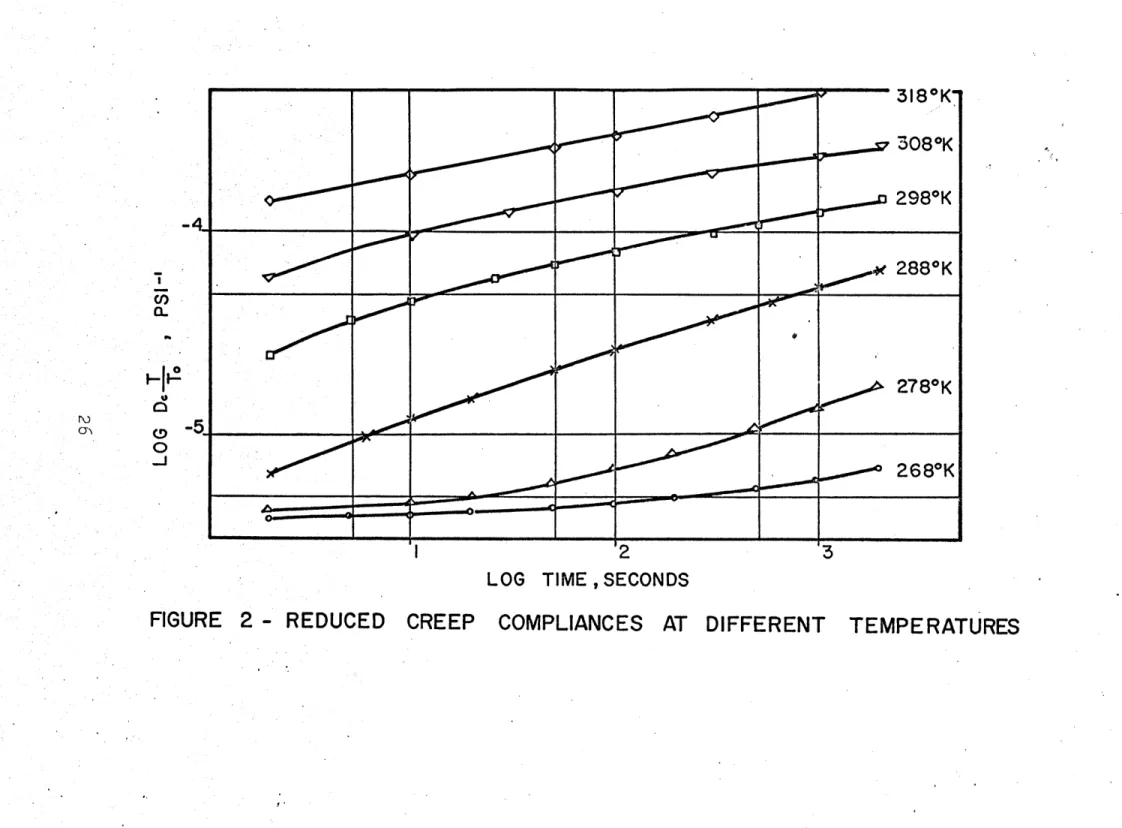
As an example of application, a sand-asphalt composite containing well graded sand and 9% by weight of a paving

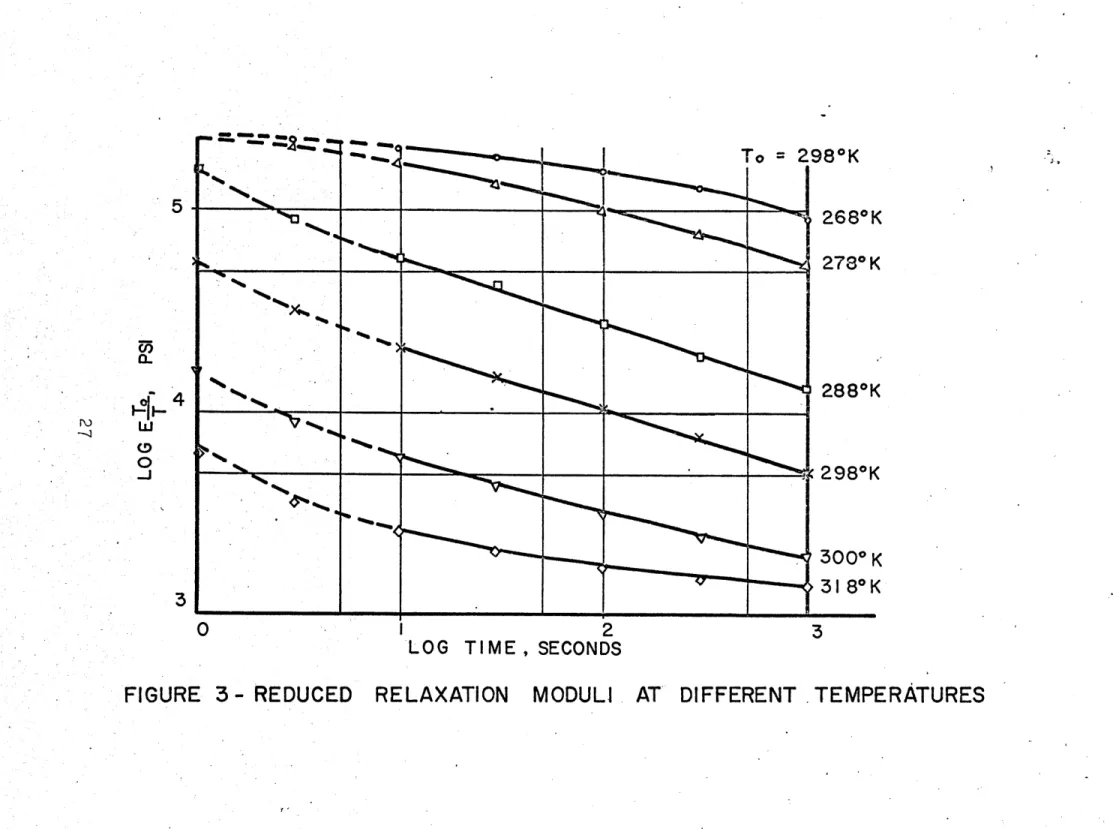
asphalt cement was used as a viscoelastic material. Cylindrical specimens were tested at different temperatures in creep and relaxation. The experimental results have shown that for

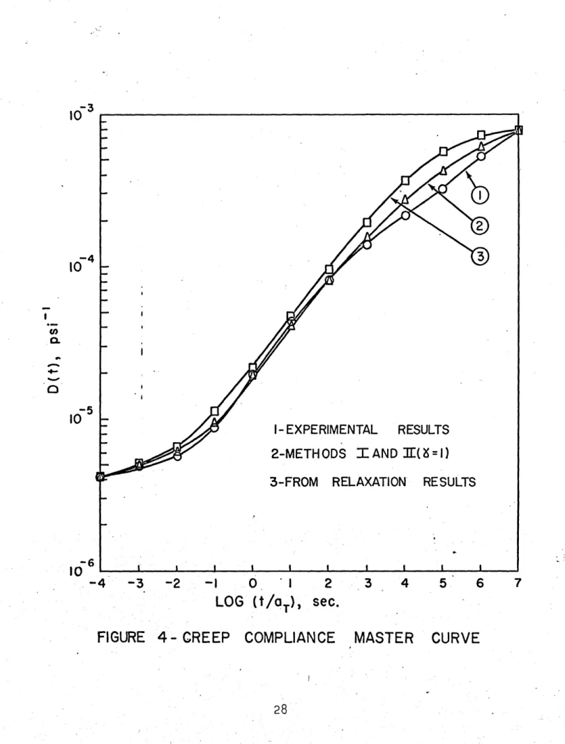
sufficiently small strains and stresses, the behavior of the material is linear and also thermorheologically simple. The experimental results from creep and relaxation are shown in Figures 2 and 3 respectively. The resulting master curves are

shown in Figures 4 and 5. The shift factor aT computed from the creep and relaxation tests is plotted in Figure 6. The

range of time for which the functions are defined is considerably greater than the experimental range. Note, however, that the shifting procedure is performed on a logarithmic scale, so that what is gained in time range may be lost in accuracy. This is

I

'2

'3

LOG TIME,SECONDS

FIGURE 2 -

REDUCED

CREEP

_{COMPLIANCES AT DIFFERENT TEMPERATURES}

0

(9 0

5

S4-O

2

LOG TIME, SECONDS

.

TEMPERATURES

3- REDUCED

o-3

10

10

10

I - EXPERIMENTAL

RESULTS

2-METH ODS

I

AND IE(6

=

I)

3-FROM

RELAXATION

RESULTS

-6

-4

-3

-2

-I

0

1

2

3

4

5

6

7

LOG

(t/oT)

sec.

A

L--4

-3

-2

-1

0

I

2

3

4

5

6

7

LOG

(t/oa),

sec.

FIGURE 5- RELAXATION

MODULUS

MASTER

29

4

S

₀

--2

-4-3.0

0

O

CREEP TEST

O

RELAXATION

TEST

3.2

3.4

3.6

I/T,

-FIGURE 6- SHIFT

3.8

4.0

FACTOR

4.2

4.4

specially true in the flat portions of the master curve where the shift factor aT is difficult to determine accurately.

2.4 Prony Series in the Analysis of Experimental Results

2.4.1 General Methods It is often convenient to describe the master curves by analytic representations. Series of

exponentials are often used for linear viscoelastic materials. For example creep and relaxation functions of those materials are generally given as

n

E(t) E= E'(t) = Xie-i 11-9

i=l

D(t) - D = D'(t) = Z (1-e t

o

i

)

II-10

i=1

where E. = lim E(t), D_O = D(O) and X_i, Zi, ai, 8_i are

con-t-*0

stants to be determined by a suitable curve-fitting technique, and E' and D' denote the transient parts of the characteristic functions. As an example, consider the determination of the transient relaxation function E' from a set of p measured values E'*(tj) = E'* at different instants tj. The 2n unknowns

J

X and ai of equation (11-9) can be obtained by using either Prony's collocation method when p=2n of Prony's least-square method when p>2n. A means to linearize the collocation and the least square methods was suggested by Schapery [351, by prescribing the value of the exponents ai. For example, in the

related to the p collocation times t. by the relation aiti=B, where the particular value =1/2 was recommended (Ref. 36

shows that for ndmerical stability 8 should be no less than 1/2), The coefficients X_i are then obtained by solving the system of linear equations.

n

-E' = X.e-ai

j

J

i=1

3

A close examination shows that this procedure is sensitive to the manner in which the exponents a. and the number of terms

1

n are chosen. An excessive smoothing of the data may result when the successive values of ai are too different in magnitude. On the other hand, alternating signs of Xi's and oscillation of the fitting curve occur when the successive values of ai are too close to each other. The system of equations (II-11) may also become ill-conditioned when several values of ai lie within a decade.

The necessity of choosing a technique that renders all the coefficients X_i or Z_i of equations (II-9) and (II-10) positive have been pointed out previously [36]. Some of the advantages ..of obtaining positive coefficients are:

a. The curvatures of functions (II-9) and (II-10) do not change sign, which.guarantees their smoothness.

b. Several mathematical transformations of equations (II-9). and II-10) are easily and accurately obtained, e.g.,

32

Laplace and Fourier transforms and their inverses. Indeed, the alternation of the signs of the coefficients causes such trans-formations to be inaccurate or even completely erroneous because series (11-9) and (II-10) are not smooth, and their first and higher order derivatives may therefore not represent the

experimental data. For example, the dynamic modulus may have negative values when some of the coefficients of series.(II-9) and (II-10) are negative.

c. If the relaxation and creep spectra H and L are introduced as in equations (11-6) and (11-7) above then the

spectra will be discrete and positive:

n

H(T)

=

Z X.6(T-a

)

11-12

i=1

where 6(T) is the Dirac delta function. The coefficients of series (II-9) and (II-10) give the amplitude of the spectra while the inverse of the exponents correspond to relaxation and retardation times respectively. This is important when the results are used to interpret the mechanical behavior of

materials.

d. It is easy to obtain a closed-form solution (cf.

boundary value problems of linear viscoelasticity, or in the

33

interconversion between creep compliance and relaxation modulus. A rule was derived in Ref. 36 to guarantee the

posi-tiveness of the coefficients Xi and Zi. This rule fixes the

minimum spacing between the ai's once the smallest ai is chosen. For the relaxation data, the collocation points must be selected

to be at least a decade apart, and to satisfy the following inequality:

1

E' > Ei+l -a) E' + 1 (a-l)2 E' i+ < n-2 11-14

i

a

i+1

a

aa

i+3'

where a=e- and E' E' = 0. The fulfillment of this rule n n+l

is a sufficient condition to assure the positiveness of the coefficients. However, this does not prevent excessive smoothing of-the data in a region where large changes occur within a decade of time. When this happens, two or more series

of overlapping collocation points may be chosen and the resul-ting series are averaged. For example, one might determine a two-terms series yl from tl and t and another two-terms series y2 from t2 and t4 and obtain a four-term series

Yerage = (Y₁ + Y2)/2. This averaging procedure may become

tedious when many series have to be used.

Furthermore, the appropriate data points necessary to satisfy inequality (II-14) may not be available in tabulated form. This is due to the fact that the choice of the col-location points depends upon preceding values selected.

~_~_~_

Therefore a more general method of characterization using an optimization technique (quadratic programming) will be

presented and its results compared with the collocation and least square techniques. Then, a method of solution of integral equations [371 is specialized to take advantage of the results of such characterization. Two examples of appli-cations demonstrate these methods.

2.4.2 Curve Fitting by the Optimization Method

This alternative curve-fitting method is formulated as a problem of minimization of a non-linear function subjected to additional constraints. This function is chosen as in a

least square method:

p

F(X) = Z w. E! - E!* 2

II-15

S

j1

and the constraints are

X_i > 0, i = 1,2, ... n

11-16

where X = [X X2...X ] and w is an appropriate weighting

function. Since viscoelastic functions may vary several orders of magnitude over the time range of interest, the choice

w =1/(E *)2 gives equal importance in the fitting to each data point.

has been solved by using a searching technique due to Flood-and Leon [38], shich is based on the general technique of Hooke and Jeeves [39].

Let F(X) be the function to minimize. A logarithmic search is made sequentially for every variable by varying it around an initial guess X0 over the positive half-axis, while

i

keeping the other variables constant. When a minimum is found, the variable is set at its new value X1 and the search proceeds

i

for the next variable. At the end of the first pass, the variables have changed from an initial value Xo to a new value X'. A search is made then along the vector (XI-Xo) to minimize F(X) and a new initial value is determined for X. The algorithm is repeated for this new initial value until a-local minimum is found, or until F(X) is judged to be small enough compared to the accuracy afforded by the data. Since the coefficients of the series have the meaning of a discrete spectrum, a fine definition of the spectrum can be obtained provided a sufficient number of data points with adequate accuracy is available.

2.4.3 _{Solution of Integral Equations by Whittaker's' Method} The representation of viscoelastic functions by Prony series (II-9) and (II-10) with positive coefficients Xi and

Z_i makes it possible to obtain a closed-form solution to

Volterra's equations of the first and,second kind which often appear in linear viscoelasticity. For example, an equation

of the first kind relates the creep and the relaxation functions:

D(T)E(t-T)dT = t II-17

o

which after differentiation reduces to an equation of the second kind

D(t) = 1 E(t-T) D(T)dT II-18

Many boundary value problems of linear viscoelasticity may also be reduced to an integral equation similar to (II-18), e.g., .see Lee and Rogers [40]. Equations (II-17) and (II-18) have

been mostly solved numerically [28 40]. However, for a certain class of kernels, which comprises Prony series of exponentials, the solution of (1I-7) and (11-18) has been given in a closed form by Whittaker [37].

To illustrate the applioability of the method, consider the determination of the creep compliance D from a relaxation modulus given by Prony series (1-9). By the application of the Whittaker's method to equation (11-18) it can be shown that: 1t D(t)

-

E

37

where

n

ji

i=l

n

j=1

jii

and the i's are the roots of the algebraic equation of

degree n in x:

n

a

7

X

+ E(O) =

II-21

i=1

n

Note that

H

(a+bj)

= (a+bl)(a+b

),..(a+bn).

j=l

Once the coefficients

Bi

are determined by solving (II-21), D

is obtained from (1-19) in the closed-form

1

nt

D(t)

CT

i=l Z (1-e

i

)

II-22

i=1

where

1 J=1 (aj-i

Z n II-23

11

(Bj-B

A.

particular case of interest is Z-

=

0 (e.g.,

uncross-linked polymers).

In this case, it appears that one of the

roots of equation (II-21) is B

=

0 and the creep compliance

reduces to:

n

Si

n

D(t) = (1 + t) + Z Z.(1-e - ) II-24

I

1=2=

which contains a term showing the presence of the Newtonian

flow.

The advantage of having positive coefficients X

appears

in the solution of the nonlinear equation (II-21).

It is

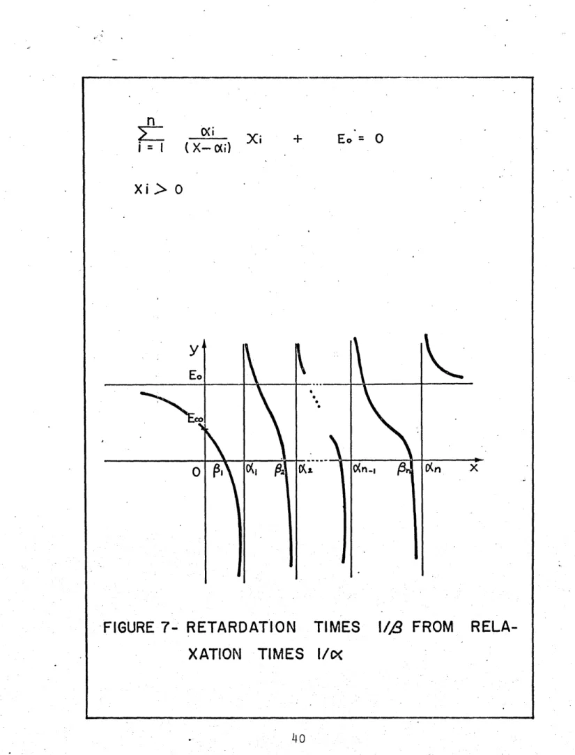
readily observed that the left hand side of equation (1-21)

ail<x<ai (see Figure 7).

Hence it is found that there are n

distinct real roots Bi's which alternate with the n values

ai's

such that 8<a"1l<

...<n<an. Thus a starting value for

every root is obtained for use in some iterative method of

solution, greatly simplifying the solution of the algebraic

equation (11-21). The Newton-Raphson method was used to

compute these roots.

Note that the role of E and D can be interchanged in

order to compute E knowing D.

2.4.4 Examples of Application

Two examples of application of the optimization method are

given. First the data generated by a 3-element model is used

to demonstrate the suitability of the curve-fitting method, and

then the method is used for the data obtained for the relaxation

of N.B.S. polyisobutylene.

In the latter case Whittaker's

n

ZI-i~I

(X-i

( X-

O(i)

+

Eo = 0

xi> 0

FIGURE

7-

RETARDATION

TIMES

1/,8 FROM

RELA-XATION

TIMES

_ _ _ __ _ _ ___ _I_ _ __ _I_ _ _I

L _ _ __~__ __

method is also applied to obtain the creep compliance from the relaxation data.

a. 3-Element Model

The minimization procedure was used to fit the data generated by a 3-element model.:

E* 2 + 10e- 0.5t 11-25

rounded to four decimal places, for 28 instant t. equally

3

spaced on a logarithmic scale between t=0.01 and t=10. A series

of the form:

28

E(tj) = 2 + X. e-i

11-26

i=l

where a. = 1/(2ti) has been adopted.

Figure 8 shows the relaxation modulus, the. theoretical relation spectrum and two approximate spectra of the 3-element model. Equation (11-26) agrees exactly within four decimal

places to the data. A sharper definition of the spectrum can

be obtained by using closely spaced exponents ai's if enough

accurate data points are provided. This possibility is shown

in Figure 8 where the effect of increasing the number of data

points results in a spectrum closer to the theoretical one.

The discrete spectra were represented by a continuous envelope

to clarify the figure.

41

0.1

1'0

TIME

T

3

ELEMENT

1.0

0*5

10

5

w

C-w

w

_w

cn

10"0

0 01

FIGURE 8-

MODEL

_:i

i :

-i

,

ii

The results obtained for the relaxation modulus of the

3-element model, using the collocation, least-square and the

minimization methods are shown in Figure 9, The collocation

method smoothes the data more than necessary when one point

per decade is used, while with two ai per decade, the three

methods yield functions that cannot be distinguished from the

data points on Figure 9. Further increase of the number of

collocation points or exponents ai to three per decade, yields

numerical instability for the collocation method, while the

least square method still produces fairly good results but

small oscillations begin to be noticeable as shown in Figure 9.

The minimization method was tried with up to 10 a. s per decade

as shown by Equation (11-26) and the results are still in

excellent agreement with the data points.

The coefficients

obtained by these different methods are presented in Table 1.

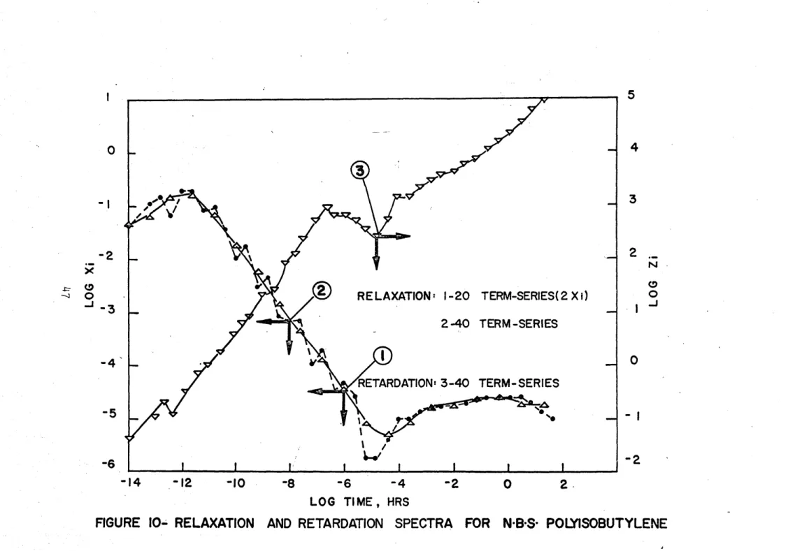
b. N.B.S. Polyisobutylene

The minimization methods were applied to the relaxation

modulus master curve of N.B.S. polyisobutylene at 25

C from

the data given in [28].

The data is given in Table 2, and

Figure 10 compares the discrete spectra obtained with a 40

terms series and a 20 terms series. With 20 terms the spectrum

is smooth while the roughness of the 40 term-series is more

likely to be due to the noise from the data, rather than due

to true properties of the material. Indeed, the 40 term-series

correspond to values of ai's more than 0.4 decade apart and it

TIME

T

FIGURE 9- COMPARISON

ELEMENT

OF

FITTING

METHODS

FOR

MODEL

TABLE 1

COMPARISON OF THE COEFFICIENTS X. DETERMINED BY THE THREE₁ CURVE FITTING METHODS

Ti = 1/2ai

..

05

0.05

0.1

0.4

0.5

0.6

0.7

1.0

5.0

10.0

Collocation

n=7

7 data points

-0,001

0.003

-0.005

10.009

-0.009

0.006

-0.004

Least square

n=7

48 data-points

-0.047

o.148

-0.182

10'.254

-0.283

0.279

-0.184

Minimization

n=28

48 data points

0.

0.

0.

0.

0.

0.

2.371

5.165

2.287

0.206

0,.

0.

0,

0.

0.

0,

45

TABLE 2

RELAXATION AND CREEP FUNCTION POLYISOBUTYLENE OF N.B.S. -log E*(t)a

log t

-14.o

-13.0

-12.0

-11.0

-10.0

0.02

0.09

0.27

0.63

1.16

1.77

2.42

3.01

3.43

3.57

3.60

3.65

3.73

3.86

4.08

4 .43

4.88

log D(1.26

0.02

0.09

0.27

0,63

1.15

1.75

2.39

2.99

3.42

3.57

3.59

3.64

3.73

3.85

4.06

4.41

4.83

Data from ref. 28

Resultsof numerical method in ref.

Results of Whittaker's method

0.02

0.09

0.28

0.71

1.36

2.01

2.68

3.19

3.48

3.57

3.60

3.64

3.73

3.86

4.09

4.51

5.14

-8.0

-6.0

-5 .0

-3.0

-2.0

-1.0

0.0

1.0

a.

b.

28

-12 -10

5

4

3

2

0

-

I

-2

-6

-4

-2

LOG TIME, HRS

FOR N.B.S- POLYISOBUTYLENE

-I

-2

-3

-4

-5

-6

-14

;;_~7=i;~- :--:~~~~*L.U-~--..~---- ---.:-.---- -'j^~.llr:lrrrr" ii--rjCj-n Yi li ----l--r

was shown in the case of the 3-element model that the

minimi-zation method was still stable when a. were 0.1 decade apart.

1

The oscillations of the spectrum which occured for the

experimental data of N.B.S. polyisobutylene, but were absent

for the 3-element model, may explain the difficulties

en-countered by Clauser and Knauss [41].

Apparently the problem

of obtaining a more refined spectrum is ill-conditioned, so

that small errors of the experimental data are amplified in

the spectrum.

Figure 11 shows the relaxation modulus of the same N.B.S.

polyisobutylene and the creep function computed by Whittaker's

inversion procedure. The results are presented in Table 2 for

comparison with the results obtained by Hopkins and Hamming [28].

A small and consistent difference is apparent in the transition

region and for longer-times in the region of viscous flow.

This difference is not significant considering .the accuracy of

the data. This is especially true for large times in the

viscous flow region where the solution may become very sensitive

to slight variations of the data, as pointed out in Reference [42].

Hence, our results tend to confirm the numerical solution of

Hopkins and Hamming, and provide simultaneously a creep spectrum

related to the relaxation spectrum. The retardation spectrum

obtained from the 40 terms relaxation spectrum is also shown

in Figure 10.

Some other advantages can be seen in Whittaker's

method like a small computing time if a good representation is

obtained with just a few terms, and the fact that all the results

5

4

-14

- 12

-10

-8

-6

-4

-2

0

2

II-

RELAXATION

ISOBUTYLENE

LOG

TIME,

HRS

DATA

AND COMPUTED

CREEP COMPLIANCE

OF

are given in an algebraic form rather-than in the form of tables.

2.5 Linearization of Results of Creep and Relaxation Functions * It was shown in section 2.2 that for a given material, the creep and relaxation functions can be obtained by a set of

independent experiments. If there are no plausible reasons to suspect that the behavior of the material would be different in creep and relaxation, then the functions E(t) and D(t) that are determined experimentally must satisfy Equation (11-3). In general, the two sets of experimental data are not going to satisfy (11-3) identically for all instants t. There are

several reasons for this inconsistency, i.e., .(a) Experimental errors.

(b) The error committed in the curve-fitting of

functions E(t) and D(t) from the experimental data. (c) For thermorheologically simple materials.

the application of the time temperature superposition principle may introduce errors that are due to the graphical shifting procedure done on a log-log scale.

This inconsistency will result in certain difficulties, for example, when one tries to obtain the dynamic creep com-pliance or relaxation modulus [251 from E(t) or D(t), one may find that the results are not unique. Furthermore, when E(t) of D(t) is used to solve boundary value problems of linear

viscoelasticity, different solutions may be obtained, depending on whether the equations of balance of momentum* are solved for

the displacement vector or the compatability equations** are solved in terms of stress functions.

Two methods that make the experimental data consistent

with the theoretical predictions are derived and an illustrative example is given.

2.5.1 Correction of Experimental Data Method I. In Time Domain

The Equation (11-3) can also be written as a Volterra

integral equation of the second kind:

E(t)D(O) = 1 - E(t-T)[D(T)/3T]dT

1-27

Let E*(t) and D*(t) be the functions that fit the experimental

data.

In general, these functions will not satisfy Equations

(1) or (2) identically. If the "deficiency" function

-f(t) = - 1 + E*(t)D*(0) + E*(t-T)[aD*(T)/3T]dT

II-28

does not

If(t)l<<1

II-29

* The relation stress

=

f(strain)is needed, i.e., E(t) has to

be given.

** The relation strain = g(stress) is needed, i.e., D(t) has

to be given.

then E(t) and D(t) are not consistent.

Since we are interested in making the experimental results consistent, it is assumed that the sought functions E(t) and D(t) are defined by

E(t) = E*(t) + El(t) = E*(t)[1 + e (t)], II-30 e

D(t) = D*(t) + D₁(t) = D*(t)[1 + vd(t)], II-31

where El(t) and Di(t) are error functions, while e (t) and Pd(t) are relative error functions. Since only the Equations (II-3) or (1-27) can be used in order to determine the two error functions, it is assumed that

d (t) e= (t) E yP(t), II-32

where y is an arbitrary real constant. Combination of (11-30), (11-31), (11-32) and (11-27) yields a nonlinear integral

equation to be solved for p(t), which was found unnecessary to be written in an explicit form. This equation is solved by a numerical procedure.

It is convenient to rewrite (II-27) as

m-i

t.+l

D(

E(tm)D(t ₎ = 1 - +1J E(tm -T)D(T - m>2

11-33

where t

and t

are, respectively, the initial and final time.

The intervals Ati=t

i+l-t

are assumed to be equal so that

g(t -tn)=g(tn). The notation g(t

mn)gm

is used hereinafter.

For the initial time (m=O), (II-3.3) reduces to EoDo=1,

which gives an algebraic equation of second degree in io whose

admissible root is

Po=(l+y)

{-1+[1-4y(1-E- 'D*-')/(1+y)2/2}/(2y)

II-34

The remaining root is physically unrealistic and will be

discarded,

By applying the mean value theorem to the integral of

(11-33), the successive values of p

are given by

.1+E. oDo.-E Do-EoD

P I = m=1, 11-35

E*Do+yEoD*

Sm=F /Gm

m>2,

-

11-36

where

)-m

mo

2

mm-1

+ 1

(E

+E

)(D -D+

,

GEm-i-1

i=1

so that the values of pi are computed by the numerical scheme (11-36)

in the sequential form

Pm=f(ml

mm-

?

'2

10 )m,2

11-37

When the spectrum of relaxation times of the material is very

wide, e.g., more than five decades, the time interval At

needed for a prescribed accuracy is so small that the amount

of computing time could be prohibitive. Therefore a somewhat

different procedure [43] has been applied that consists in

evaluating Vi up to some time t

with equal time intervals

At =t

/n, where n is the number of intervals. The interval

At

is then multiplied by an integer k>l and the computations

pj,

times t2jjkAtl=jAt

for j<n/k. The same procedure is repeated

until the desired value of tm is reached. The choice of n

and k can be made by running numerical experiments in the

computer for different values of n and k. This numerical

procedure is applicable if the memory of the material fades

in time. Thus, in order to have sufficient accuracy in the

computations, it is only necessary to have a finer mesh for

the last two or three decades of time, rather than in the total

time interval [t0,t].

Method IT. Correction in Laplace Domain

EL(p)DL(p) = 1

where

EL(p)=p,

E(t) exp(-pt)dt

11-39

JO

denotes the Laplace transform of E(t).

Combining Equations

II-30II-31 & 11-38 we obtain

[EL (p) + EL (p)][D (p)

+

DIL (p)]

=

1,

II-40

where E1L(p), D1L(p) are the Laplace transforms of the error

functions El, Di.

To avoid the indeterminancy, it is assumed

that ElL and .DL

are related in the Laplace domain by the

relative error function

v(p)

E1L(p)/E*(p)

(1/y)D L(p)/D,(p)

II-41

It should be noted that this assumption is similar but not

identical to the one used in Method I. The two functions v(t)

and p(t) are not identical even if the same weighting factor y

is used in both methods.

Equations 11-40 & II-41yield an algebraic equation of

the second degree in v(p), whose acceptable root is

v(p)

=

[l+y)/2y]{-1+[1-4yE(p)(l+y)-

_{1/2 }}

_II-42

e(p) =1 - [E*(p) D*(p)]-

1

EL(p) = E*(p)[l+v(p)],

DL(P) = D (p)[l+yv(p)]

To simplify the computation of E* and D*, it

L L' is assumed that

the experimental relaxation modulus can be approximated by

II-45

E*(t) = E +

E

where X and a. are known constants and E. is the equilibrium value. A similar assumption. is adopted for D*(t).

v(p), EL(p) and

DL(P)

Equations (II-42)-(II-44).

E(t) = E* +

can be readily computed using

It is further assumed that

n

E

X

exp(-iit),

such that

where E is computed from the values E* (p) and D* (p) for

p 0.

The unknown coefficients X. of Equation (11-46) can be

1

determined by satisfying Equation (II-47) at n values of p.=2a. where

so that

I-43

II-47

for j=1,2...n. This yields the system of linear equations

n

E [pj/(i+j)] Xi EL (PjE j=1,2...n

11-8

i=l

for the unknowns X

The relative error function pe(t) that

results from this method can be easily computed using Equations

II-30,II-45 & II-46.

The same procedure can be repeated for

the compliance D(t).

2.5.2

Optimization

To avoid the arbitrariness of y, some functional of the

two error functions El(t) and Di(t) should be minimized with

respect to y. To do this, the integral of the sum of the

squares of the error functions E

and E

in the Laplace domain

is used. This functional is given by

F(y)

which can be written as

-(l+y 2 (+y) 2

F

( y )

4 -_

Z

(l+y 2 )v2(p,y)dp

II-49

II-50

CX

{2

4y

s(p)

2

[l

Y(p),1/2}dp

It is not difficult to show that F(y) is a minimum in the

Laplace domain when y=l, which is equivalent to assuming equal

relative errors for the two series of tests.

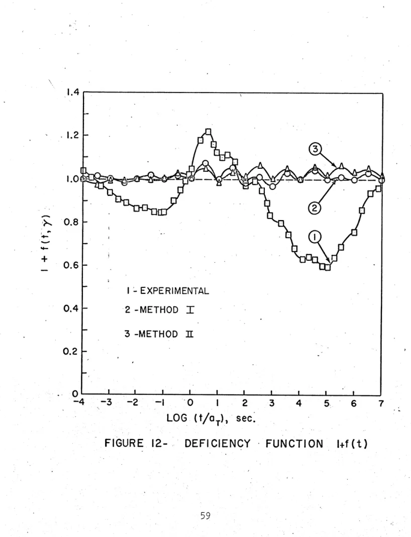
2.5.3 An Example of Application

The experimental results obtained in Reference 44 for

a sand-asphalt mixtures and described in section 2.3 are here.

The curve fitting of the measured relaxation and creep

functions are performed using Equation (II-45).

To check the consistency of the experimental results, the

relaxation and creep functions have been computed using Hopkins

and Hamming's method [28], and are shown in Figures 4 and 5.

Moreover, the deficiency integral (1-29) was also evaluated

numerically by using the scheme

f(tn) = -1+E*(tn )D(0)

n-1

-1 [E*(t i ) + E*(t i+l )][D*(tn-ti+)-D*(tn-ti)] II-51 i=l

and it is represented in Figure 12.

The inconsistency of the

data is apparent, the large values of f(t) in the transition

region can be attributed to one or several .factors mentioned

previously. Therefore, both methods described in the previous

section are applied to the experimental data using y=l.

.The function p(t) computed with Method I is shown in

Figure 13 for different numbers of intervals n. The numerical

results show that p converges towards a unique solution for

sufficiently large values of n.

When method II is applied to the same data, the resulting

error functions pe (t) and Pd(t) that are computed from E

(t),

E*(t) and D

(t), D*(t) compare well with p(t), as shown in