Computational techniques in
propagation-based x-ray phase imaging
The MIT Faculty has made this article openly available.
Please share
how this access benefits you. Your story matters.
Citation
Petruccelli, Jonathan C., et al. "Computational Techniques in
Propagation-Based x-Ray Phase Imaging, Proceedings of SPIE
9209, Advances in Computational Methods for X-Ray Optics III, 17-21
August, 2014, San Diego, California, edited by Manuel Sanchez del
Rio and Oleg Chubar, 2014, p. 92090P. © 2014 SPIE
As Published
http://dx.doi.org/10.1117/12.2062917
Publisher
SPIE
Version
Final published version
Citable link
http://hdl.handle.net/1721.1/119146
Terms of Use
Article is made available in accordance with the publisher's
policy and may be subject to US copyright law. Please refer to the
publisher's site for terms of use.
PROCEEDINGS OF SPIE
SPIEDigitalLibrary.org/conference-proceedings-of-spieComputational techniques in
propagation-based x-ray phase
imaging
Jonathan C. Petruccelli, Sajjad Tahir, Sajid Bashir, Adam
Pan, Lei Tian, et al.
Jonathan C. Petruccelli, Sajjad Tahir, Sajid Bashir, Adam Pan, Lei Tian,
Ling Xu, C. A. MacDonald, George Barbastathis, "Computational techniques
in propagation-based x-ray phase imaging," Proc. SPIE 9209, Advances in
Computational Methods for X-Ray Optics III, 92090P (17 September 2014);
Computational techniques in propagation–based x–ray phase
imaging
Jonathan C. Petruccelli
1, Sajjad Tahir
1, Sajid Bashir
1, Adam Pan
2, Lei Tian
3, Ling Xu
2,
C. A. MacDonald
1and George Barbastathis
2,4,51
Department of Physics, University at Albany – State University of New York,
1400 Washington Avenue, Albany, NY 12222, USA
2
Department of Mechanical Engineering, Massachusetts Institute of Technology,
77 Massachusetts Avenue, Cambridge, MA 02139, USA
3
Department of Electrical Engineering and Computer Sciences, University of California,
Berkeley CA 94720, USA
4
Shanghai Jiao Tong University – University of Michigan Joint Institute
800 Dong Chuan Road, Minhang District, Shanghai 200240, China
5
Singapore–MIT Alliance for Research and Technology (SMART) Centre,
1 Create Way, Singapore 138602, Singapore
ABSTRACT
X–ray phase imaging utilizes a variety of techniques to render phase information as intensity contrast and these intensity images can in some cases be processed to retrieve quantitative phase. A subset of these techniques use free space propagation to generate phase contrast and phase can be recovered by inverting differential equations governing propagation. Two techniques to generate quantitative phase reconstructions from a single phase contrast image are described in detail, along with regularization techniques to reduce the influence of noise. Lastly, a recently developed technique utilizing a binary–amplitude grid to enhance signal strength in propagation–based techniques is described.
Keywords: Phase retrieval, transport of intensity, x–ray imaging, grid–based phase imaging, partial coherence,
polycapillary optics
1. INTRODUCTION
Since their discovery by R¨ontgen in 1895, x-ray imaging has found widespread use where noninvasive imaging of the internal structure of opaque objects is required. In traditional radiography, the contrast in the captured image is generated by differential attenuation within the object. However, in many cases of interest, e.g. imaging soft tissue in a medical setting or discriminating between water and non-nitrogenous liquid explosives in airport baggage screening,1 structures of interest consist of materials that present similar attenuation and for these
applications, x ray imaging has found limited use.
In the past two decades there has been considerable work on x-ray phase imaging techniques, which leverage the fact that x rays are not only attenuated by a sample, but acquire a phase associated with the optical path length acquired in transition through the sample. Phase imaging can often provide significantly enhanced contrast over attenuation–based imaging. However, detectors directly measure intensity of x rays, not phase. Attenuation through a sample is immediately apparent by a corresponding decrease in intensity at the sample’s output face. However, phase is not available from this intensity measurement. Instead, phase imaging systems require careful design in order to ensure that a phase signature is present in measured intensity. This has led to a variety of proposed systems for x-ray phase imaging.2 The gold standard in phase imaging is interferometry, where phase information is rendered in interference patterns between a reference beam and a beam with unknown phase.3
Further author information: (Send correspondence to Jonathan Petruccelli) Jonathan Petruccelli: E-mail: [email protected]
Invited Paper
Advances in Computational Methods for X-Ray Optics III, edited by Manuel Sanchez del Rio, Oleg Chubar, Proc. of SPIE Vol. 9209, 92090P · © 2014 SPIE
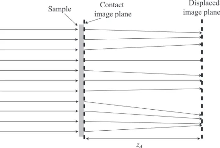
Contact image plane Displaced image plane Sample zd
Figure 1. Refraction of x rays by a thin phase sample. Incident x rays propagating from left to right are bent as a result of phase accumulated by traversing the sample. In the contact plane immediately after the sample, these rays have not moved transversely with respect to their initial positions. However, at a displaced plane a distance zd from the sample,
the refraction of x rays results in some detector regions receiving a higher density of x rays and therefore measuring a higher intensity as a result of phase.
However, these fringes are sensitive to vibrations and are typically used with high brilliance sources in systems with a high degree of vibration isolation such as synchrotron imaging. An alternative family of techniques that do not have nearly this level of vibration sensitivity rely principally on the fact that phase variation across the sample refracts incident x rays at an angle proportional to phase gradient. One can directly measure x rays within a narrow angular window by finely tuning an analyzer crystal, thus characterizing phase through the angles of rays emerging from a sample.4, 5 Another widely studied technique is to use a pair of gratings: the first grating patterns an incident beam with a known phase pattern.6 In the absence of a sample, this phase pattern creates a Talbot image at a precise distance. The Talbot image is quite sensitive to phase and can be disrupted by phase imparted by a sample. However, as the grating spacing is typically smaller than a detector pixel and so an analyzer grating of fine pitch is used to measure changes in the Talbot image due to phase.
In what follows, we consider what is perhaps the simplest method of phase contrast: the use of propagation to render phase visible. If x rays that have been refracted by a sample phase are allowed to propagate some distance away from the sample, ray deflection angle and therefore phase can be rendered as intensity contrast on the detector as illustrated in Fig. 1. Therefore, by displacing the detector and measuring intensity, one can generate a phase–contrast image. If the goal is to recover a quantitative phase profile of the beam immediately after the sample, it is possible to compute ray refraction angle and then phase from the contact and displaced detector images.
2. PHASE AND OPTICAL PATH LENGTH
In order to use phase imaging to obtain useful information about a sample of interest, one must have a model relating the phase of the x–ray beam to sample properties. A coherent beam whose main axis of propagation aligns with the z axis can be expressed (after factoring out a linear term of the form exp(i2π/λz) in complex form as
U (x, z) =√I(x, z) exp[iϕ(x, z)], (1) where x denotes a point in a plane transverse to the z axis, where I denotes intensity and ϕ the phase of the beam. For such a beam, phase imaging means designing an optical system in such a way that ϕ is rendered in an intensity profile. In many cases, the phase profile of the beam is approximately known, as is the case for plane waves or cone beams, and one is interested in measuring changes to this beam’s phase induced by propagation through a sample. For many cases of interest where the sample is thin and interacts relatively weakly with the beam, a weak–scattering approximation can be made, in which case the influence of the sample on the beam can be approximated by integration of the sample’s refractive index along rectilinear ray paths through the sample.
Consider a sample whose exit face is located at z = 0 that can be characterized by the complex–valued refractive index
n(x, z) = 1− δ(x, z) + iβ(x, z) (2) that is illuminated by a monochromatic plane wave aligned with the optical axis. The phase difference between rays that have traversed the sample and those that have passed through air (n ≈ 1) is proportional to the projection of δ through the sample
ϕ(x, 0) =−k
∫
δ(x, z) dz, (3)
where the integral is taken between entrance and exit planes bounding the sample, k = 2π/λ is the wave number and λ the wavelength of the x rays. The intensity immediately after the sample is given by I(x, 0) which includes attenuation of the primary beam by absorption given by exp(−2k∫β dz) and scattering. If the incident beam
cannot be approximated as a plane wave, the integrals must be taken over the appropriate ray trajectories traced through the object. In what follows, we will work from this approximation, that the phase we seek to retrieve is the projection of δ through the object.
3. TRANSPORT OF INTENSITY PHASE IMAGING
Propagation of a monochromatic beam described by a complex field of the form Eq. (1) is governed by the paraxial wave equation
∂ ∂zU (x, z) = i 2k∇ 2 xU (x, z), (4)
where ∇x denotes a 2D Laplacian in the transverse plane and k = 2π/λ is the wavenumber with λ being the
wavelength of the beam. Polychromatic beams may be constructed by integrating over the spectrum, though we will neglect this as the requirement of monochromaticity is relatively lax in x–ray phase imaging.2 Since Eq. (4) is differential equation for the complex–valued field U , propagation of U depends both on I and ϕ and this equation describes the relationship between intensity and phase upon propagtion. The relationship between intensity and phase can be rendered more obvious by explicitly decomposing Eq. (4) into real and imaginary parts, yielding ∂ ∂zI(x, z) +∇x· { 1 k[I(x, z)∇xϕ(x, z)] } = 0, (5a) ∂ ∂z { 1 k[I(x, z)∇xϕ(x, z)] } =−1 k2∇x· [I(x, z)∇xϕ(x, z)⊗ ∇xϕ(x, z)] + I(x, z)∇x ( ∇2 x √ I(x, z) 2k2√I(x, z) ) , (5b)
where ⊗ denotes the dyadic product between two vectors and k = 2π/λ. These formulations are valid for a beam propagating any distance and contain the same physics as Eq. (4). However, they are not widely used in practice as it is typically easier to work with a linear equation in complex–valued field than with a pair of coupled, nonlinear differential equations in real–valued intensity and phase.
If we are concerned with recovering phase from closely spaced intensity measurements, we can employ only Eq. (5a), which is a linear differential equation for ϕ provided I can be measured. In order to solve this equation the derivative of I along the z axis can be approximated from closely spaced images using finite differences. For hard x rays, such distances are often on the order of half a meter. Equation (5a) is called the transport of intensity equation (TIE).7 Notice that this same approximation arises from taking the geometrical optics limit
of Eqs. (5) where only terms to first order in k−1 are retained. This also amounts to assuming that the term in curly brackets in Eqs. (5), which describes ray direction, does not change appreciably over distances considered. The TIE is often used in the form of Eq. (5a) for visible light microscopy systems, in which case three images are generally acquired: one in–focus image used on the right–hand side of the equation and two defocused images acquired on either side of the focus to approximate the derivative of I along z. For x–ray phase imaging without optical elements, the TIE is often recast using forward differences to relate I at a distance zdfrom a sample from
I at the exit face of the sample as illustrated in Fig. 1, I(x, zd)≈ I0(x)−
z
Object Detector z o zd Point source h Mh Object Detector z o z d Extended source xs xi
(a)
(b)
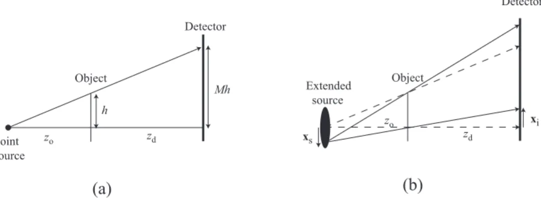
Figure 2. (a) Imaging with a point source illustrating magnification of an object of height h to height M h at the detector. (b) Blurring of image due to finite source size. Dashed lines indicate rays emitted from an on–axis point on the source while solid lines indicate rays from a source point located at axial coordinate xs. The corresponding image point shift for
this off–axis source point is xi=−(zd/zo)xs.
where I0 and ϕ0 denote phase at the exit face of the sample, respectively. The second term on the right–hand
side of Eq. (6) is associated with phase contrast due to deflection of rays at an angle|∇xϕ0|/k, from which it is
clear that phase contrast will be strongest at sharp edges in phase. From a computational standpoint, this equation can be rearranged as
g = Aϕ0, (7)
where
g =−k
z[I(x, zd)− I0(x)] , (8)
Aϕ0=∇x· [I0(x)∇xϕ0(x)] . (9)
this is now a linear equation where the left–hand side of the equation may be entirely expressed in terms of measured values and the right–hand side is an operator of the form ∇x· I∇x acting on the unknown phase.
Techniques for solving linear systems can be invoked to recover phase from this set of images.
These derivations assume that imaging is being performed with a collimated beam of x rays. In practice, a cone beam is often used, which can be idealized as coming from a perfect point source of x rays. In this case, a modified form of the TIE holds, where the images and propagation distances must be scaled to account for magnification.8, 9 If the image is magnified by M = (z
o+ zd)/zo where zo is the source-to-object distance and
zd is the object-to-detector distance as illustrated in Fig. 2(a)
I(M x, ∆z)≈ I0(x)−
z
kM∇x· [I0(x)∇xϕ0(x)] , (10)
where x denotes coordinates in the object plane. Finally, note that while Eq. (10) relates propagated phase to a contact image, a similar equation can be derived to relate intensity in any two closely spaced planes to the phase in the initial plane.
3.1 The TIE and partial coherence
The TIE, like other x ray phase contrast techniques, is fairly insensitive to temporal coherence, i.e. a beam from a broad spectrum source. However, the TIE, like all phase imaging techniques, is highly sensitive to spatial coherence. For tabletop systems, this is generally achieved by using a small source spot placed some distance from the object.
Because the TIE using a pure point source is a geometrical optics model and tabletop x ray sources can generally be considered fully incoherent primary sources, the effect of a finite source spot can be accounted for
by purely geometrical blurring of the image by the finite size of source. (More general states of coherence require a more sophisticated model.10, 11) Consider a primary source spot emitting x rays that is located a distance z
o
from the object. The source can be approximated as consisting of a continuous distribution of intensity Is(x).
Since the source is assumed to be nearly perfectly incoherent, x rays from neigboring points will not interfere on the detector so that we can simply sum the images produced by each source point to obtain the total image. If the source point is displaced from the optical axis by an amount xs, the corresponding image point will be
displaced by an amount xi =−(zd/zo)xs as illustrated in Fig. 2(b).
Each point on the source produces a TIE image of the form Eq. (11), shifted by an amount−zd/zoxs, the
net image at the detector is a convolution with the source intensity Is(−zo/zdx). For a fixed source spot size,
the amount of blurring induced by the convolution can be reduced by increasing the source–to–object distance
zo or decreasing the object–to–detector distance zd. The former also reduces the total intensity captured at the
detector while the latter reduces the strength of the TIE phase contrast signature, both of which undermine the image quality. Therefore, the most practical method of producing high quality TIE images is to use a small source spot, generally of 25 µm or less in radius.
The results presented in what follows use two different types of sources to obtain a small spot. In the first case, a microfocus x ray source (Hammamatsu L812103) was used to directly generate a small primary source of x rays. A second option that we have investigated is the use of a standard tabletop source with a primary spot size too large to allow phase contrast imaging, but which is used in conjunction with a focusing polycapillary optic. The focusing optic is capable of focusing the x ray beam down to a secondary spot of the required size for phase imaging.12
3.2 Single shot techniques
The form of TIE presented in Eq. (11) assumes that two images are obtained: one in the contact plane and one at a distance zdfrom the contact plane. In many cases it is impractical to take multiple of images while displacing
the detector. In hard x-ray phase imaging where phase contrast fringes are on the order of 100 microns wide, precise alignment and image registration are required. This has proven extremely challenging and so a variety of single-shot techniques have been proposed.13 In this section, two are described in detail.
In the first, one assumes a weakly attenuating object such that I0(x) ≈ I0 = constant. In this case, the
transport of intensity equation reduces to
∇2 xϕ0(x)≈ g = − M k zd [ I(M x, z) I0(x) − 1 ] , (11)
which is Poisson’s equation relating phase to measured intensity. For simplicity, we denote the right–hand side of the equation as g, which depends entirely on measured intensity and known constants. I0can either be measured
a priori or it can be determined from the mean intensity of a background patch in the acquired image. This technique is particularly simple as Poisson’s equation can be solved efficiently with fast Fourier transform (FFT) techniques. The major limitation of this technique is that realistic objects present non–zero attenuation. This can introduce significant error into the reconstruction which appears as a “halo” of phase around an object due to the the weak–attenuation (WA) approximation attributing intensity variations due to attenuation entirely to phase. If significant intensity variation is attributable to attenuation, the reconstructed phase is not expected to be accurate.
Another limitation of this technique is the amplification of low–frequency noise in the reconstructed image. Since intensity variations are attributed to the Laplacian of phase, large signal is attributable to high phase Laplacian, which is associated with sharp features in the phase. Slowly varying features in phase generate a very weak signal in the measured image. Therefore, in inverting the problem to recover phase, one must preferentially amplify low spatial frequencies (associated with slowly varying phase features) over high spatial frequencies. This preferentially amplifies low spatial frequency noise as well, resulting in a “blotchy” appearance to the recovered phase. In Fourier space, WA phase retrieval can be expressed as
ϕ0=−F−1 [ 1 (2π)2|u|2F(g) ] , (12)
whereF denotes a Fourier transform and F−1 an inverse Fourier transform such that
F[f(x)] = ˜f (u) =
∫∫
f (x) exp(−i2πx · u) d2x (13)
F−1[ ˜f (u)] = f (x) =∫∫ f (u) exp(i2πx˜ · u) d2u, (14)
where u is spatial frequency. The Fourier transform allows the Laplacian to be replaced by multiplication by
−(2π)2|u|2. Solving for phase involves decomposing the measured data g into Fourier components, amplifying
these components by−(2π)−2|u|−2, which preferentially amplifies low spatial frequencies (diverging to infinity at |u| = 0), and inverse Fourier transforming to recover the phase image in the spatial domain. In order to avoid the
problematic amplification of low–frequency noise, one typically introduces regularization to seek a solution that both closely matches the measured data and contains physically reasonable structures. For example, one could choose Tikhonov regularization which tends to minimize the total integrated magnitude of phase (∫∫|ϕ(x)|2d2x).
Since low spatial frequencies generate large regions of non–zero phase, this regularization tends to remove low spatial frequencies in the reconstructions. Thikonov regularized WA phase retrieval has a closed form solution
ϕ0=−F−1 [ (2π)2|u|2 (2π)4|u|4+ ϵ2F(g) ] , (15)
where ϵ is a regularization parameter that is chosen to damp low spatial frequency components in the reconstruc-tion as illustrated in Fig. 3. While Tikhonov regularizareconstruc-tion does remove low frequencies from the reconstrucreconstruc-tion, it does not attempt to discriminate between low frequency signal and noise components in the phase. For rela-tively large regularization parameters, all low spatial frequencies are essentially removed from the reconstruction, resulting in a reconstructed phase that resembles the phase-contrast image. Reducing the regularization parame-ter makes the phase reconstruction more accurate but results in a “blotchy” reconstruction due to low–frequency noise amplification. Note that since this technique erroneously attributes all attenuation effects to phase and that attenuation exhibits features on the scale of the object size, some of the error introduced by this approx-imation can be removed by Tikohonov regularization. This is evident in the reduced halo around the object when ϵ = 10−4 compared to ϵ = 10−5. Alternative regularizers can be employed to preserve some low frequency content in the reconstructed phase.14
A second single–shot technique called phase–attenuation duality (PAD) makes the assumption that the at-tenuation is dominated by Compton scattering, which can be safely assumed for high energy (≤ 60 keV) x rays imaging low atomic number (Z < 9) elements. Even for lower beam energies, PAD can often yield reasonably accurate results as will be demonstrated in what follows. In this case, attenuation through the sample is approx-imately proportional to phase as both are proportional to projected electron density through the sample. The exact proportionality constant depends on the mean wavelength of the x rays, but can be readily calculated. The contact image can be expressed as
I0(x) = exp [ 2ϕ(x) γ(λ) ] , (16)
where γ is a proportionality constant between attenuation and phase. The contact intensity is no longer an independent unknown, but depends on the unknown phase.15 Plugged into Eq. (11) this results in
g = I(M x, z) = [ 1−zλγ(λ) 4πM ∇ 2 x ] I0(x). (17)
This can again be readily inverted in the Fourier domain as
I0(x) =F−1 { F[g(x)] 1 + Γ|u|2 } , (18)
where Γ = πzλγ(λ)/M . If needed, phase can be found from
ϕ(x) = γ
−4 0 −10 0 −45 0 −450 0 −30 True phase 0
Weak attenuation phase reconstructions
ε=10-2 ε=10-3
ε=10-5
ε=10-4
Phase contrast image
Figure 3. Weak–attenuation phase reconstruction simulation of a 1 mm diameter poly(methyl methacrylate) (PMMA) sphere assuming a monochromatic, 30 keV x-ray beam. Phase contrast image simulated at a distance of z = 0.5 m from sample with effective pixel size (demagnified to the object plane) of 10 µm. (Top left) The true phase of the simulated object and (bottom left) simulated measured intensity (phase contrast image) with Poisson noise. Four reconstructions of phase are shown to the right with varying regularization parameter ϵ.
Notice that while this still amplifies low–spatial frequency components preferentially, these are no longer amplified without bound as |u| → 0. This tends to alleviate the need for regularization, although one could still use Tikhonov regularization to further suppress low frequency amplification if necessary.
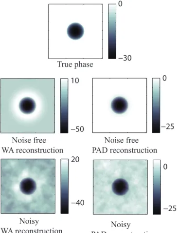
To demonstrate the features of this approximation and phase reconstructions, phase imaging was simulated for a poly(methyl methacrylate) (PMMA) sphere assuming a 30 keV x–ray beam and a detector with effective pixel size (demagnified to the object plane) of 10 µm as illustrated in Fig. 4. Propagation distance zdwas 0.5 m and the
source size was assumed to be small enough that any blurring could be neglected. Phase contrast was simulated using wave propagation and reconstruction was performed using both Tikhonov regularized (ϵ = 10−4.5) WA phase retrieval and PAD, both with and without added Poisson noise. Phase attenuation duality performs considerably better as an approximation at this energy and requires no regularization.
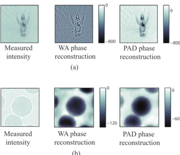
Experimental results are illustrated in Fig 5(a) using a focusing polycapillary optic to create a virtual source size of 25 µm.16 To exaimine the performance of this system for phase imaging of tissue, an insect was imaged.
Source–to–object distance was zo = 25 cm while object–to–detector distance was zd = 75 cm. Effective pixel
size using an image plate was 12.5 µm in object coordinates. The x ray was operated at a voltage of 45 kVp. The results clearly illustrate improved contrast and reduced noise in the phase reconstructions. Figure 5(b) illustrates similar reconstructions of polyethylene microspheres using a Hammamatsu L812103 microfocus source operated at 40 kVp. In this case, distances were zo = 32 cm, zd = 160 cm and effective pixel size using an
Andor Ixon EMCCD was 2.67 µm. Since we know a priori that these are spheres, δ can be determined from the phase images. For WA phase retrieval, δ≈ 8.2 × 10⁻⁷ while for PAD, δ≈ 4.8 × 10⁻⁷. The expected value of δ for polyethylene at this energy is approximately 4.2× 10⁻⁷, again indicating that PAD is the more accurate approach.
4. GRID–BASED IMAGING
The right–hand side of the forward–difference form of the TIE with a point source can be expanded as
I(M x, zd)− I0(x)≈ − zd kMI0(x)∇ 2 xϕ0(x)− zd kM [∇xI0(x)]· [∇xϕ0(x)] . (20)
The first term on the right–hand side describes the phase contrast produced by interaction of varying object attenuation with varying phase. The second indicates phase contrast produced purely by phase. The WA
−30
0
−50
10
−25
0
−40
20
−25
0
True phase
Noise free
WA reconstruction
Noise free
PAD reconstruction
Noisy
WA reconstruction
PAD reconstruction
Noisy
Figure 4. Single image phase reconstruction simulation of a 1 mm diameter poly(methyl methacrylate) (PMMA) sphere. (Top center) True phase of the simulated object. The four figures appearing below demonstrate phase reconstruction for both noise–free and noisy simulations using Thikonov regularized WA and PAD methods, as indicated.
approximation to TIE assumes that intensity variation is negligible compared to phase variation, eliminating the first term. However, we can intentionally introduce a mask with strong intensity variation G(x) shortly before or after the object such that total intensity immediately after the object/mask combination is I0(x)G(x). If the
variation in G is much larger than the variation in I0 or ϕ0, then terms not containing derivatives of G can be
neglected, yielding
I(M x, zd)≈ G(x)I0(x)−
zd
kMI0(x) [∇xG(x)]· [∇xϕ0(x)] , (21)
which again is a second–order, linear, partial differential equation for ϕ0 which can be solved provided I0, G
and I(x, z) are known. The mask transmittance G is generally known a priori and I(x, z) is measured by the detector. This leaves I0 and ϕ0 as unknowns, and as in the case of traditional TIE without a mask, either
multiple images or strong assumptions on I0 and ϕ0 such as the WA or PAD approximations are required.
However, it is possible to rapidly isolate I0and phase from a single image taken with the detector at position
zd if one uses a periodic grid.17 Consider a grid of period Λ then the G can be expanded in a Fourier series
G(x) = ∞ ∑ n=−∞ cnexp ( i2πn Λ gˆ· x ) , (22)
where ˆg is a unit vector pointing in the direction perpendicular to the grid lines. Inserting this form of G into
Eq. (21), and Fourier transforming the result, one obtains
F(I)(u) ≈ ∞ ∑ n=−∞ cnδ2 ( u−nˆg Λ ) ∗ [ F(I0)(u)− i(2π)2zd λΛ nˆg· F(I0∇xϕ)(u) ] , (23)
−800 0 −800 0 Measured intensity WA phase reconstruction PAD phase reconstruction Measured intensity WA phase reconstruction PAD phase reconstruction (a) (b) −120 0 −60 0
Figure 5. Single image phase reconstruction using experimental data. (a) The raw intensity image of an insect captured using a focusing polycapillary optic to generate source along with Tikhonov regularized WA (ϵ = 10−4.5) and PAD reconstructions. (b) The raw intensity image of polyethylene microspheres captured using a microfocus source along with Tikhonov regularized WA (ϵ = 10−4) and PAD reconstructions.
I0 from 0th order harmonic DPC image from 1st order harmonic DPC image from 2nd order harmonic c Raw image
Figure 6. Grid–based imaging of 2 mm glass spheres.
where ∗ denotes convolution with respect to u. Convolution with the delta function localizes the quantity in square brackets about each harmonic in the Fourier domain. If the signal is narrow band enough so that information from neighboring harmonics does not overlap, information from the nth harmonic can be isolated by windowing in the Fourier domain, shifted back to the origin, and inverse Fourier transformed, yielding
In(x) = cn [ I0(x)− i(2π)2zd λΛ nI0(x)ˆg· ∇xϕ(x) ] . (24)
The grid itself can be imaged in the absence of an object to characterize cn, ˆg, and Λ. Then the term I0(x)
can be extracted from the n = 0 harmonic. Once I0 is known, the n = 1 harmonic can be used to obtain the
differential phase contrast (DPC) image of ˆg∇xϕ. Higher order harmonics can be used to improve the DPC
image.
As an example of this technique, consider a 2 mm glass bead imaged with a Rh source operating at 35 kVp.18 No focusing optics are used and the source spot size is roughly 50 µm. The source–to–object and object–to– detector distances are given by zo= 9.5 cm and zd= 51.5 cm. The grating is placed 31.5 cm after the object and
20 cm before the detector. Without the grating present, phase contrast is not visible at the detector. By placing the grating in the path of the beam, I0and differential phase contrast (DPC) images, IDPC= ˆg· ∇xϕ(x) can be
obtained as illustrated in Fig. 6. Note that although ϕ0could in principle be retrieved from IDPC, reconstructions
5. CONCLUDING REMARKS
This manuscript has described several techniques for propagation–based phase imaging based on the transport of intensity equation as well as discussing the role of computational phase retrieval from raw images. It also described the effect of introducing a grid into propagation–based phase imaging. As mentioned previously, these are not by any means the only models describing propagation–induced phase contrast. A variety of alternative models exist, including the contrast transfer function technique (for weak phase objects at longer propagation distances),19 and Born and Rytov scattering–based models.20 Interferometric techniques and analyzer crystal
based techniques have also proved useful for phase imaging.
Computational techniques often rely on phase reconstruction from a single image. Although weak attenuation and phase–attenuation duality methods have been described here, other single–shot techniques exist, including single and dual–material approximations which are similar in function to phase attenuation duality (in assuming that phase and attenuation are proportional for each material).13 Furthermore, a great deal of recent work
has been done on implementing phase tomography, where the goal is to find the volumetric distribution of δ rather than the projected phase through an object. Tomographic reconstructions can benefit strongly from the use of regularization techniques, since most object of interest consist of discrete structures of single materials, and therefore one expects to find a phase reconstruction consisting of regions of constant δ and can choose a regularization technique to seek solutions of this form.21–23
6. ACKNOWLEDGEMENTS
Portions of this work were supported by the Department of Homeland Security, Science and Technology Direc-torate through contract HSHQDC-11-C-00083 and by the National Institutes of Health (NIH) through project number R01EB009715.
REFERENCES
[1] Singh, S. and Singh, M., “Explosives detection systems (EDS) for aviation security,” Signal Process. 83, 3155 (2003).
[2] Momose, A., “Recent advances in x-ray phase imaging,” Jpn. J. Appl. Phys. 44, 6355-6367 (2005). [3] Bonse, U. and Hart, M., “An x-ray interferometer,” Appl. Phys. Lett. 6, 155–156 (1965).
[4] Somenkov, V. A., Tkalich, A. K., and Shil’shtein, S. S., “Refraction contrast in x-ray introscopy,” Sov. Phys.
Tech. Phys. 36, 1309–1311 (1991).
[5] Davis, T. J., Gao, D., Gureyev, T., Stevenson, A. W., and Wilkins, S. W., “Phase-contrast imaging of weakly absorbing materials using hard x-rays,” Nature 373, 595–598 (1995).
[6] Pfeiffer, F., Weitkamp, T., Bunk, O., and David, C., “Phase retrieval and differential phase-contrast imaging with low-brilliance x-ray sources,” Nat Phys 2, 258–261 (2006).
[7] Reed Teague, M., “Deterministic phase retrieval: a green’s function solution,” J. Opt. Soc. Am. 73, 1434– 1441 (1983).
[8] Gureyev, T. E. and Wilkins, S. W., “On x-ray phase imaging with a point source,” J. Opt. Soc. Am. A 15, 579–585 (1998).
[9] Paganin, D., [Coherent X-Ray Optics ], Oxford University Press (Jan. 2006).
[10] T. E. Gureyev, Y. I. Nesterets, D. M. Paganin, A. Pogany, and S. W. Wilkins, “Linear algorithms for phase retrieval in the Fresnel region. 2. Partially coherent illumination,” Opt. Commun. 259, 569-580 (2006). [11] Petruccelli, J.C., Tian, L., and Barbastathis, G., “The transport of intensity equation for optical path length
recovery using partially coherent illumination,” Opt. Express 21, 1094-4087 (2013).
[12] MacDonald, C. A., “Focusing polycapillary optics and their applications, x-ray optics and instrumentation,”
X-Ray Focusing: Techniques and Applications 2010, 867049 (2010).
[13] Chen, R. C., Rigon, L., and Longo, R., “Comparison of single distance phase retrieval algorithms by considering different object composition and the effect of statistical and structural noise,” Opt. Express 21, 7384–7399 (2013).
[14] Tian, L., Petruccelli, J., and Barbastathis, G., “Nonlinear diffusion regularization for transport of intensity phase imaging,” Opt. Lett. 19, 4131–4133 (2012).
[15] Wu, X., Liu, H., and Yan, A., “X-ray phase-attenuation duality and phase retrieval,” Opt. Lett. 30, 379–381 (2005).
[16] Bashir, S., Tahir, S., MacDonald, C. A., and Petruccelli, J. C., “Phase imaging using polycapillary optics,”
SPIE Advances in X-Ray/EUV Optics and Components IX (2014).
[17] Bennett, E. E., Kopace, R., Stein, A. F., and Wen, H., “A grating-based single shot x-ray phase contrast and diffraction method for in-vivo imaging,” Med Phys. 37, 6047–6054 (2010).
[18] Tahir, S., Bashir, S., MacDonald, C. A., and Petruccelli, J. C., “Fourier transform image processing tech-niques for grid-based phase imaging,” SPIE Advances in Computational Methods for X-Ray Optics III (2014).
[19] Guigay, J. P., Langer, M., Boistel, R., and Cloetens, P., “Mixed transfer function and transport of intensity approach for phase retrieval in the fresnel region,” Opt. Lett. 32, 1617–1619 (2007).
[20] Gureyev, T. E., Davis, T. J., Pogany, A., Mayo, S. C., and Wilkins, S. W., “Optical phase retrieval by use of first born- and rytov-type approximations,” Appl. Opt. 43, 2418–2430 (2004).
[21] Sidky, E. Y., Anastasio, M. A., and Pan, X., “Image reconstruction exploiting object sparsity in boundary-enhanced x-ray phase-contrast tomography,” Opt. Express 18, 10404–10422 (2010).
[22] Tian, L., Petruccelli, J. C., Miao, Q., Kudrolli, H., Nagarkar, V., and Barbastathis, G., “Compressive x-ray phase tomography based on the transport of intensity equation,” Opt. Lett. 38, 3418–3421 (2013).
[23] Pan, A., Xu, L., Petruccelli, J. C., Gupta, R., Singh, B., and Barbastathis, G., “Contrast enhancement in x-ray phase contrast tomography,” Optics Express 22, 18020 (2014).