Comparison and Financial Assessment of Demand Forecasting Methodologies for
Seasonal CPGs
by
Burak Gundogdu, BS, MBA and
Jeffrey Maloney, BS
SUBMITTED TO THE PROGRAM IN SUPPLY CHAIN MANAGEMENT IN PARTIAL FULFILLMENT OF THE REQUIREMENTS FOR THE DEGREE OF
MASTER OF APPLIED SCIENCE IN SUPPLY CHAIN MANAGEMENT AT THE
MASSACHUSETTS INSTITUTE OF TECHNOLOGY JUNE 2019
© 2019 Burak Gundogdu and Jeffrey Maloney. All rights reserved.
The authors hereby grant to MIT permission to reproduce and to distribute publicly paper and electronic copies of this capstone document in whole or in part in any medium now known or hereafter created. Signature of Author: ____________________________________________________________________
Department of Supply Chain Management May 10, 2019 Signature of Author: ____________________________________________________________________ Department of Supply Chain Management
May 10, 2019 Certified by: __________________________________________________________________________ Tugba Efendigil Research Scientist Capstone Advisor Accepted by:__________________________________________________________________________ Dr. Yossi Sheffi Director, Center for Transportation and Logistics Elisha Gray II Professor of Engineering Systems Professor, Civil and Environmental Engineering
1
Comparison and Financial Assessment of Demand Forecasting Methodologies for
Seasonal CPGs
by
Burak Gundogdu and Jeffrey Maloney
Submitted to the Program in Supply Chain Management on May 10, 2019 in Partial Fulfillment of the
Requirements for the Degree of Master of Applied Science in Supply Chain Management
ABSTRACT
Forecast accuracy is an ongoing challenge for made-to-stock companies. For highly seasonal fast-moving consumer packaged goods (CPGs) companies like King’s Hawaiian, an improved forecast accuracy can have significant financial benefits. Traditional time series forecasting methods are quick to build and simple to run, but with the proliferation of available data and decreasing cost of computational power, time series’ position as the most cost-effective demand forecasting method is now in question. Machine learning demand forecasting is increasingly offered as an improved alternative to traditional statistical techniques, but can this advanced analytical approach deliver more value than the cost to implement and maintain? To answer this question, we created a three-dimensional evaluation (cube search) across five unique models with varying pairs of hyper-parameters and eight different data sets with different features to identify the most accurate model. The selected model was then compared to the current statistical approach used at King’s Hawaiian to determine not just the impact on forecast accuracy but the change in required safety stock. Our approach identified a machine learning model, trained on data that included features beyond the traditional data set, that resulted in a nearly 4% improvement in the annual forecast accuracy over the current statistical approach. The decrease in the value of the safety stock as a result of the lower forecast variation offsets the incremental costs of data and personnel required to run the more advanced model. The research demonstrates that a machine learning model can outperform traditional approaches for highly seasonal CPGs with sufficient cost savings to justify the implementation. Our research helps frame the financial implications associated with adopting advanced analytic techniques like machine learning. The benefits of this research extend beyond King’s Hawaiian to companies with similar characteristics that are facing this decision.
Capstone Advisor: Tugba Efendigil Title: Research Scientist
2
ACKNOWLEDGMENTS
We would like to thank the community of the Supply Chain Management program at MIT for giving us a once in a lifetime experience to work with and learn from such inspiring people. We are especially grateful to our advisor, Dr. Tugba Efendigil, for her leadership and insight throughout this project. This project would not have been possible without the support and participation of the sponsoring company, King’s Hawaiian. A special thanks to the leadership at King’s Hawaiian; Mark, John, Dan, Tony and Joe, whose vision and commitment to employee development and knowledge have made this project a reality. We would also like to thank the King’s Hawaiian o’hana who have contributed to this project and
graciously lent support when called upon: Nicolas, Bill, DG, Jordan, and Amelia. Burak & Jeff
I am honored to have worked on this project with a partner as talented as Burak and thank him for his patience and the knowledge he has gifted me throughout this process. I am truly grateful to my friends and family who have supported me on this adventure. I’m sure Burak feels the same.
Jeff
I would like to thank my imaginary cat “Schroding-cat” for always being there, or not. Burak
3 TABLE OF CONTENTS Abstract ……….… 1 Acknowledgments ...………..………... 2 Table of Contents …...………...… 3 List of Figures ………...……… 5 List of Tables ……… 5 1 Introduction ……… 6 1.1 Motivation ……….………..…...… 6 1.2 Problem Statement ……….……….7 1.3 Summary of Methodology ……….……….……... 8 1.4 Company Background ...……….………... 9 2 Literature Review ……….………....….... 10 2.1 Overview ……….……….… 10
2.2 Machine Learning in Time Series Forecasting ……….……….……... 10
2.3 Studies in Traditional and Machine Learning Based Demand Forecasting ………... 11
2.4 Studies Focusing on FMCG Demand Forecasting with Machine Learning ……….… 12
3 Data and Methodology ……….……….…………... 14
3.1 Data Collection ..……….………..……...… 17
3.1.1 Shipment Data from Internal ERP ……….………..….… 17
3.1.2 Statistical Forecast Data from Internal Model ….……….… 17
3.1.3 Safety Stock from Internal Model ….……….……….. 18
3.1.4 Consumption Data from External Vendor ….………...… 19
3.1.5 Population Data from External Database .………..….. 20
3.1.6 Climate Data from External Database .……….………… 20
3.2 Data Exploration .……….…...…. 21
3.2.1 Summary Statistics …...……… 21
3.2.2 Seasonality ….……….…. 22
3.2.3 Severe Weather Data ….……….….. 24
3.2.4 Census Data ….………...……….… 24
3.3 Data Pre-Processing ….………...…….… 26
3.3.1 Aggregation ….……… 26
3.3.2 De-Seasonalizing ….………...….… 27
3.3.3 Aligning by State ….……….… 29
3.3.4 External Attribute Incorporation ….……….… 29
3.3.5 Data Partitioning ….………. 29 3.4 Data Scrubbing ….………..…………..… 30 3.4.1 Temporal Alignment ….……….…………..… 30 3.4.2 Product Specific ….……….….… 30 3.4.3 Regionality ….……….. 31 3.4.4 Weather ….……….……….…. 31 3.4.5 Census ….………. 31 3.4.6 Data Cleansing ….……….……..……. 32 3.5 Data Normalization ….………. 32
4
3.6 Feature Selection and Engineering ….………..… 32
3.7 Machine Learning Models ….……….….… 33
3.7.1 Random Forests (RF) ….……….…………. 33
3.7.2 Artificial Neural Networks (MLP) ….……….. 34
3.7.3 Support Vector Machines (SVR) ….………...…………. 34
3.7.4 Gradient Boosting (GB) ….……….……….… 35 3.7.5 K-Nearest Neighbors (KNN) ….………..…………..……….. 35 3.8 Performance Measurement ….………...……….……. 35 3.8.1 Forecast Error ….………..… 35 3.8.2 Financial Impacts ….………...…….… 37 4 Results ….………. 37 4.1 Feature Selection ….……….… 38 4.1.1 All Features ….………. 38 4.1.2 Baseline ….……….………. 38 4.1.3 Feature Select 1 ….………..….… 38 4.1.4 Feature Select 2 ….………..….… 39 4.2 Model Selection ….……….…. 39
4.2.1 Cube Search Process Results ….……….……….. 40
4.2.2 Cube Search Performance Results ….……….………. 41
4.3 Selected Model ….………...……….… 54
4.3.1 Model, Features, and Hyperparameters ….…………...………...…. 55
4.4 Forecast Accuracy ….………..……….… 56
4.4.1 Error Measurement ….……….… 56
4.4.2 Error Comparison to Statistical ….………..…….… 57
4.5 Inventory and Financial Impact ….……….…………..… 58
5 Conclusions ….………. 60 5.1 Feature Selection ….……….… 60 5.2 Model Selection ….……….……….… 61 5.3 Financial Impact ….……….……….… 62 5.4 Further Investigation ….………..………….… 63 References ….………..…………...… 64
5
LIST OF FIGURES
Figure 3.1: Data Sources and Process Map ………..………...… 15
Figure 3.2: Cube Search Process Flow ………..……….….… 16
Figure 3.3: Visualization of Safety Stock ………..………..… 19
Figure 3.4: Heat Map of Total Shipments ………..………. 23
Figure 3.5: Shipments, De-seasonalized ………..………..……. 27
Figure 3.6: Consumption, De-seasonalized ………..………... 28
Figure 3.7: Current Network Level Forecast Performance ………..………..….. 36
Figure 3.8: Current Statistical Forecast Regional Forecast Performance ………...….… 36
Figure 4.1: Feature Importance Curve ………..………... 39
Figure 4.2: Comparison of Model Run Time ………..……….… 40
Figure 4.3: SVR Grid Search Results ………..………....… 42
Figure 4.4: SVR Epsilon Hyper-parameter Performance Curve ……….………..…….……….… 43
Figure 4.5: SVR C Hyper-parameter Performance Curve ………..……….… 43
Figure 4.6: MLP Layers Hyper-parameter Cross Performance Results ………...……….… 44
Figure 4.7: RF Grid Search Results ………..………..…….… 45
Figure 4.8: RF Max Features Hyper-parameter Performance Curve ………..…………..…..… 46
Figure 4.9: RF Max Depth Hyper-parameter Performance Curve ………...………..………….… 47
Figure 4.10: GB Grid Search Results ………..………...…. 48
Figure 4.11: GB Min Sample Split Hyper-parameter Performance Curve ……….………. 49
Figure 4.12: GB N-Estimator Hyper-parameter Performance Curve ………...…..……….… 49
Figure 4.13: KNN Grid Search Results ………..……….… 50
Figure 4.14: KNN P Hyper-parameter Performance Curve ………..………..……….… 51
Figure 4.15: KNN N-Neighbors Hyper-parameter Performance Curve ………....…………..… 52
Figure 4.16: Comparison of Error from Cube Search ………..………..….… 53
Figure 4.17: Comparison of Train-Test Variance ………..………. 54
Figure 4.18: KNN Seasonal vs De-Seasonalized Performance ………..………. 55
Figure 4.19: Geographic Distribution Regions ………..………..… 57
Figure 4.20: Comparison of Safety Stock levels for Statistical vs Machine Learning ………...…. 59
LIST OF TABLES Table 2.1: Literature Overview ………..………... 13
Table 3.1: Shipment Data Attributes ………..……….… 17
Table 3.2: Statistical Forecast Attributes ………..………..….… 18
Table 3.3: Consumption Data Attributes ………..………..….… 20
Table 3.4: Summary Statistics for Shipment Actuals ……..………..………..………… 21
Table 3.5: Summary Statistics for Consumption Actuals ………..……….. 22
6
1. INTRODUCTION
1.1 Motivation
For businesses that operate from a demand forecast, achieving a low forecast error can allow them to carry less safety stock and confers a significant financial advantage. Conversely, a high forecast error requires greater investment in safety stock inventory to cover demand variation. High levels of safety stock can become debilitating for small firms that do not possess adequate financial strength and may pose a barrier to entry into markets for new firms. A high forecast error can lead to missed sales and be detrimental to customer relationships and ultimately damage the brand.
High forecast errors also lead to supply chain inefficiencies. Companies can suffer from increasing logistics costs due to relocating product throughout the network and shipping product from a sub-optimal region for a higher cost. Forecast volatility causes a bullwhip effect upstream to manufacturing, which can result in operational inefficiencies through frequent adjustments to production plans. The higher volatility complicates upstream planning with vendors, resulting in inefficient order sizes and increased costs for expedited orders.
Improving forecast accuracy is a challenge that many companies face. It is especially important to consumer packaged goods (CPG) companies that are built-to-stock, as they must invest in finished goods to cover forecasted demand while minimizing their financial exposure. Build-to-stock companies that have strong seasonal demand must begin planning and building inventory earlier, and with less information, than similar non-seasonal CPG companies.
Advancements in forecasting software and analytics have provided modern businesses with many options. The promise of advanced forecasting methods is a more accurate forecast that will yield financial savings to the firm by reducing forecast error and uncertainty. However, advanced forecasting techniques require an investment in not just the software, but the increased amounts of data required to run the model. Additionally, the company must account for the cost of the increasingly sophisticated personnel
7 responsible for initializing and maintaining an advanced demand forecasting solution. A company must select a forecast process that matches their demand pattern while being cognizant of the ongoing costs for forecast software and all supporting processes. The development of a framework that can narrow the selection process based on potential financial impact can help companies invest capital in a solution that is sized for their business model.
Many companies currently face just such a challenge. As a highly seasonal build-to-stock business, King’s Hawaiian must rely on a forecast to build inventory sufficient to cover their peak demand and carry safety stock to ensure high customer service levels. Forecast accuracy becomes even more important when additional constraints such as capacity, obsolescence, and seasonality are considered. Forecast-driven companies like King’s Hawaiian need to understand whether they can expect to see an appreciable decrease in forecast error from the adoption of a machine learning forecast. They also need to understand whether the potential savings, resulting from reduced safety stock due to a lower forecast error, will offset the increased costs of data and technical expertise.
1.2 Problem Statement
Many methodologies for demand forecasting are available to companies. Traditional methods include, but are not limited to, expert opinions, market research, and statistical methods (which are typically built in Excel) to better understand trends in the marketplace.
One alternative to traditional methods is applying machine learning to demand forecasting. Even though this is hardly a new idea, advanced machine learning techniques have only recently started to take their place in supply chain professionals’ toolbox. That change can mainly be attributed to the recent rise of artificial intelligence/machine learning applications’ popularity in supply chain management due to the potential profitability (Chui et al., 2018) and the increased ease of access and implementation of complex machine learning models with new techniques and software (e.g. more than fifty thousand Tensorflow repositories on Github as of January 2019).
8 The main question we will answer in this capstone project is whether the improvement (if any) in demand forecast accuracy from a machine learning process versus traditional statistical methods is significant enough to justify the increased costs.
While machine learning methods have been heavily researched, there is a lack of academic studies on the financial link between the benefit and costs of applying machine learning to demand forecasting.
Therefore, we will demonstrate an approach that can help companies make cost-effective decisions when it comes to implementing a machine learning forecast, in addition to determining which machine learning methods provide the best results and what data to include in the models for companies similar to King’s Hawaiian.
1.3 Summary of Methodology
The approach for this capstone is to identify, through current academic literature, existing machine learning methods used for demand forecasting. We compared these techniques to the current statistical method being used at King’s Hawaiian.
Since machine learning models can leverage large amounts of information, data in addition to King’s Hawaiian’s historical shipments was incorporated. In addition to the shipment data out of the ERP system, third-party consumption data that are being purchased were also used. To augment the machine learning, publicly available data sets for socio-economic factors (e.g. income, education level) and severe weather events such as hurricanes or winter storms were also captured. The relative values of these additional data attributes were classified by machine learning to determine the relevancy of incorporating the information in the demand forecast.
Five different machine learning demand forecasting methodologies -- support vector regression, artificial neural network, random forest, gradient boosting, and k-nearest neighbors regression -- were run over multiple iterations with various attributes to generate many demand forecasts. The accuracies of these models were compared to the current statistical model and evaluated using standard forecast error metrics.
9 When a solution was found that generated a lower forecast error than the current statistical methodology, the change in projected safety stock as a result of the new forecast error was calculated. The resulting financial savings were compared against the incremental costs for the additional data, technical and personnel-related costs required to generate a forecast through more technologically advanced techniques. This comparison allowed for the evaluation of the net savings that can be expected from safety stock reduction, for a similar company, as a result of adopting a machine learning demand forecast.
1.4 Company Background
King’s Hawaiian is a national Hawaiian Foods company with a primary focus on dinner rolls. A national producer of consumer goods, King’s Hawaiian is a family owned and operated business that was started as a bakery and restaurant in Hilo, Hawaii in the 1950s. King’s Hawaiian entered the mass-produced CPG stage in the 1970s with the opening of their first production facility in Torrance, California. Today King’s Hawaiian operates on both coasts with three production facilities and a national sales footprint (King’s Hawaiian Marketing Department, 2019).
King’s Hawaiian is a highly seasonal consumer product, most popular during the Thanksgiving,
Christmas, and Easter holiday seasons. They contract a network of frozen warehouses and carriers to store and deliver their product to national retailers and redistributors. As a build-to-stock company, King’s Hawaiian relies heavily on its Sales and Operations Planning process to correctly align its production capabilities with the forecasted demand (King’s Hawaiian Supply Chain Department, 2019).
To deliver on its brand promise of being irresistible, King’s Hawaiian ensures a 99.5% service level by holding safety stock to cover the volatility in the demand forecast. As the company continues to grow, both in sales and unique offerings for customers, the utilization of their facilities increases. The above-mentioned factors increase the pressure for an accurate forecast to deliver product to its customers while minimizing the amount of capital invested as safety stock for the seasonal demand peaks.
10
2. LITERATURE REVIEW
2.1 Overview
Machine learning is a very broad topic and a very dynamic area of research where new techniques are continuously being developed. For that reason, the general academic approach in the studies we have examined is comparing a few select machine learning techniques to traditional approaches. We also came across some broader comparative studies, but they are limited in number and by no means include all possible machine learning approaches.
The general consensus is that machine learning based methods are promising in improving demand forecasts even if they do not necessarily perform better than traditional methods under every scenario. The challenge for demand forecasters is finding out which machine learning methods can perform better than the legacy approaches for the underlying demand of their specific industry and product, and how to make sure that the improvement in forecasts is significant enough. Even though some papers mention that applying machine learning is costlier than staying with traditional methods, e.g. by sharing computation times, we did not come across a study that implements a detailed cost-benefit analysis of using machine learning to improve supply chain demand forecasts.
We also noticed that there is no consistency in terms of terminology. A good example is the classification of linear regression as both a machine learning based technique and also a traditional method due to its wide usage both in academia and industry. In this section, we followed the academic authors’
classification of methods.
2.2 Machine Learning in Time Series Forecasting
Artificial intelligence in general and machine learning specifically are highlighted as having significant potential to improve costs over traditional analytical techniques (Chui et al., 2018). The field of supply chain management and the consumer packaged goods industry are identified as among the best candidates for adoption of these techniques, projecting some of the largest cost savings as a result. The cases Chui et al. reviewed for demand forecasting that implemented artificial intelligence to identify underlying causal
11 drivers show a 10-20 percent improvement over existing methodologies. While acknowledging challenges around these more advanced methods, they conclude that there is a clear argument for the value of
augmenting existing analytical capabilities with machine learning and artificial intelligence.
Ahmed, Atiya, Gayar, & El-Shishiny (2010) applied multiple machine learning models to M3 time series competition data to compare the major models using approximately a thousand time series and argue that multilayer perceptron and the Gaussian process regression perform better than Bayesian neural networks, radial basis functions, generalized regression neural networks (kernel regression), k-nearest neighbors regression, CART regression trees and support vector regression.
Even though machine learning is considered a very promising field in improving time series forecasting, some studies argue that they will not consistently improve over the forecasts using traditional techniques. Makridakis, Spiliotis, and Assimakopoulos (2018) find that post-sample accuracy of traditional methods is better than that of machine learning methods for all forecasting horizons examined using 1045 M3 competition time series.
2.3 Studies in Traditional and Machine Learning Based Demand Forecasting
Many authors have applied machine learning to demand forecasting and compared forecast accuracy against the accuracy of traditional forecasting methods. Hribar, Potocnik, Silc, & Papa (2018) show that recurrent neural networks are more accurate than empirical models in forecasting natural gas demand, and they suggest implementing a linear regression model instead when computational resources are limited. Machine learning based demand forecasting using recurrent neural networks and support vector machines can show better performance than traditional techniques (naïve forecasting, trend, moving average, and linear regression), but it should be noted that improvement in forecast accuracy with those more complex models is not always more statistically significant than using linear regression (Carbonneau, Laframboise, & Vahidov, 2008). Saloux and Candanedo (2018) also argue that advanced machine learning approaches – decision trees, support vector machines, artificial neural networks – improve demand forecasts
12 Machine learning based demand forecasting can also be used to improve forecasts when demand is intermittent. Neural networks can perform better than Croston, moving average and single exponential smoothing when demand is irregular, as in spare parts supply chain (Amirkolaii, Baboli, Shahzad, & Tonadre, 2017). Vargas and Cortes (2017) claim that artificial neural networks perform well in the sample period, but they are less steady than ARIMA in post-sample period forecasting of irregular spare parts demand.
For a demand forecaster who agrees that machine learning based demand forecasting can perform better than traditional approaches, the next challenge is to pick the right machine learning technique. Therefore, part of the literature surveyed focuses on comparing machine learning methods with each other. Gaur, Goel, and Jain (2015) implement a simulation using Walmart shipment data set and a confusion matrix as a performance metric to compare nearest neighbors and Bayesian networks for demand forecasting in supply chain management and argue that the latter performs better. Guanghui (2012) implements support vector regression and radial basis function neural networks to forecast demand of weekly sales for a large paper enterprise and shows that support vector regression performs better. In a study comparing three machine learning approaches to forecast demand of bike-sharing service, linear regression performs better than neural networks and random forests, although using a longer time period than the one-month used in the study (i.e. more data) is suggested to understand real performance of more complex approaches. Combining multiple techniques to build ensemble or hybrid models is also common when implementing machine learning in general. Efendigil, Onut, and Kahraman (2009) use an adaptive neuro fuzzy inference system to utilize both neural networks and fuzzy modeling to get more accurate demand forecasts.
Johansson et al. (2017) use ensembles of machine learning algorithms for operational demand forecasting and argue that extreme learning machines provide the best accuracy.
2.4 Studies Focusing on FMCG Demand Forecasting with Machine Learning
Forecasting demand for fast moving consumer goods (FMCG) is challenging due to reasons like shelf-life and seasonality. For the same reasons, this is an area where applying machine learning techniques can result in better forecasts as machine learning models can capture complex relationships. The studies we
13 have analyzed regarding applying machine learning to demand forecasting of FMCG products show promising results. While a large selection of machine learning algorithms has been implemented, neural networks and support vector machines are among the common ones. Table 2.1 summarizes papers that generally focus on demand forecasting of different FMCG products and summarizes the methods and features used along with the conclusions.
Table 2.1: Literature Overview. Review and summary of similar demand forecasting studies
Research into the application of machine learning in the field of demand forecasting is still in its early stages and has shown mixed results. There is no one-size-fits-all approach when it comes to replacing traditional demand forecasting methods. The selection of the machine learning model, and the hyperparameters that guide it, play a significant role in the final forecast accuracy.
Title Forecasted FMCG product / industry Methods Features Conclusion
A Comparative Study of Machine Learning Frameworks for Demand Forecasting (Mupparaju, Soni, Gujela,
Lanham, 2018) Grocery store items
Moving average, gradient boosting, factorization machines, three versions of deep neural networks
Sales, date, store and item numbers, promotion, store location, categorization, clustering, family item and class, perishability
Neural network model with a sequence-to-sequence approach to forecast the sequence of 16-day sales using the sequence of previous 50-day sales as input performs best
A comparison of sales forecasting methods for a feed company: A case
study (Demir and Akkas, 2018) Five products of a feed company
Moving average, exponential smoothing, Holt's linear method, Winters's method, artificial neural
networks, support vector regression Product sales
Support vector regression produces the best results
A Comparison of Various Forecasting Methods for Autocorrelated Time Series (Kandananond, 2012)
Demand of six different products from a consumer product company (e.g. dishwasher liquid, detergent)
Artificial neural network (multilayer perceptrons (MLP) and radial basis function (RBF)), support vector machine (SVM), and autoregressive integrated
moving average (ARIMA) Historical demand at t-1, t-2,..., t-10
Support vector machines perform better than ARIMA and artificial neural networks
Artificial Neural Networks/or Demand Forecasting: Application Using Moroccan Supermarket Data (Slimani, El
Farissi, Achchab, 2015) Supermarket sales
Focuses on finding the optimal Multi Layer Perceptron (MLP) structure for
demand forecasting Daily order quantities
MLP with hidden layers 4, 4, 4 performs best
Forecasting Seasonal Footwear Demand Using Machine Learning (Liu and Fricke,
2018) Footwear
Regression trees, random forests, k-nearest neighbors, linear regression and neural networks
Store count, month, lifecycle month, gender, AUR, year, basic material, MSRP, color, lifecycle, cut description, product class description
Ensemble methods (median and average) and random forests gave the best predictive performance Oral-Care Goods Sales Forecasting Using
Artificial Neural Network Model
(Vhatkar and Dias, 2016) Oral-care
Back-Propagation Neural Network
Model Past sales
Neural network models can be used for predicting the sales of FMCG products Predictive Demand Models in the Food
and Agriculture Sectors: An Analysis of the Current Models and Results of a Novel Approach using Machine Learning Techniques with Retail Scanner Data (Pezente, 2018)
Sugar commodity demand (utilizes products with sugar component)
Linear regression, ARIMA, artificial neural networks
Consumption, price, volume, GDP, population
Neural netrowk models were significantly more accurate Support Vector Regression for
Newspaper/Magazine Sales Forecasting
(Yu, Qi, Zhao, 2013) Newspaper/magazines
Traditional regression, support vector regression
Store type, occupation, education, age, gender, and income
Support vector regression performs better
Utilizing Artificial Neural Networks to Predict Demand for Weather-Sensitive Products at Retail Stores (Taghizadeh,
2017) Weather-sensitive retail products
The multilayer perceptron, time delay neural networks, recurrent neural networks, bagging, linear regression
Sales of potentially weather-sensitive products, weather
The multilayer perceptron (MLP) with the back propagation learning algorithm performs best
Sales forecasting using extreme learning machine with applications in fashion retailing (Sun, Choi, Au, Yu,
2008) Fashion products
Batch steepest descent backpropagation algorithm with an adaptive learning rate (GDA), the gradient descent momentum and adaptive learning ratio backpropagation (GDX), extreme learning machine (ELM) and extreme learning machine extension (ELME)
Sales data of one kind of fashion
14
3. DATA AND METHODOLOGY
This section discusses the collection, preparation, and analysis of the various data sources required for the machine learning demand forecast. The goal was to selectively and iteratively evaluate relevant regional data to increase the predictive performance of a machine learning forecast, which required processing and aligning the data from internal and external data sources. Sources, features, and level of resolution of the different data sources were identified.
Also detailed is the preparation of the different data sources including aggregation, normalization, standardization, and feature selection using the random forest machine learning model, for input into the various machine learning forecast models. The different machine learning models (support vector regression, artificial neural network, random forest, gradient boosting, and k-nearest neighbors regression), hyper-parameters and feature sets evaluated are discussed, as well as the methodology for measuring their performance against the current Holt-Winters statistical forecast. The overall process is mapped out in Figure 3.1.
15 Fig. 3.1 Data Sources and Process Map. Data sources, and path of data for forecast generation and
comparison
Every model underwent a combinatorial evaluation for each of the two hyper-parameters selected, as well as each feature attribute set identified, resulting in search across not just the two dimensions of the hyperparameters but the third dimension of the feature attribute set as well. The cube search process is detailed in Fig 3.2
ERP Shipment Data - Product Type - Date/Time - Seasonality Calendar - Quantity Shipped - Geographic Attributes Consumption Data - Product Type - Date/Time - Price - Quantity Sold - Geographic Attributes Census Data - Geographic attributes - Population attributes - Household attributes - Income attributes - Ethnic attributes - Education attributes Climate Data - Geographic attributes - Calendar attributes - Severe climate Characteristics Data Exporation - Statistical Characteristics - Trends, variation and seasonality - Outliers and exceptions
Data Pre- Processing - Filter out aggregated accounts - Restrict data to those present in both shipment and consumption data sets - Aggregate data to weekly level - Aggregate data to state level
Data Cleansing - Clean and Standardize Data - Impute Missing Data with Averages - Drop SKUs with insufficient history
Feature Engineering - Random Forest
- Management Expertise
Machine Learning Models - Neural Net (MLP) - GB
- SVR - KNN
- Random Forest
Performance Measurement - Forecast Error: Regional & Annual - Mean R2
- Weighted Absolute Percent Error
Financial Impact - Change in Safety Stock Investment - Comparison of Savings vs Model Cost
16 Fig 3.2 Cube Search Process Flow. The data flow in the Cube Search methodology as data moves from
pre-processing through model selection to final validation and analysis
1
Cleaned Data
Select Feature 1 Model
Feature Selector
RF Feature SelectorManagement Exploratory Model
Analysis
Baseline All Select Feature 2 Model List Hyper-Parameter ranges
Split Data
Cube Search (Parameter 1,
Hyper-Parameter 2, Feature Set) with 3-Fold Cross Validation
For every Model
Results of Cube Search
Final Model Validation on Test
Data
Y Train X Train X Test
Transformed X Test Data Transformation Pipelines Transformed X Train Data Y Test Fit, Predict Model Custom Loss
Function Financial AnalysisInventory, Process
Function ObjectData 2D Visual
17
3.1 Data Collection
3.1.1 Shipment Data from Internal ERP
Shipment data from King’s Hawaiian ERP system, MAS500, were collected and housed in an internal SQL data table. These data reflected the units sold to retail customers, not end consumers. Shipment data have the attributes identified in Table 3.1.
Table 3.1 Shipment Data Attributes
Data Source Attribute Description
Shipment Data SKU Unique Product Number
Shipment Data
Replacement
SKU Closest Active SKU to Historical SKU
Shipment Data Quantity Units, or Pounds, Shipped
Shipment Data Customer Name of Account Receiving Product
Shipment Data Ship To Receiving Address of Customer
Shipment Data 3PL Unique Warehouse Designator
Shipment Data Ship Date Day, Week, Month, Year
Shipment Data Seasonal ID Identifier Based on Historic Seasonality
Historical shipment data are the primary data source for the current King’s Hawaiian statistical forecast. Six years of historical data (2013 to 2018) were available in the data warehouse. The shipment data comprise 372,074 records, from 58 unique active SKUs from 45 states. The seasonal ID was assigned based on historical shipment demand related to national holidays that had differential volume of shipments. The duration of elevated shipments, lull periods afterward, as well as the offset from the holiday, were also identified. The data set was restricted to have SKUs that are no longer sold, or have been re-launched, to align to current SKU IDs (Replacement SKU) to preserve the validity of historical records.
3.1.2 Statistical Forecast Data from Internal Model
The current statistical forecast methodology in use at King’s Hawaiian is a Holt-Winters model. The forecast was built from historical shipment data going back to 2012, when available. The data set that was
18 fed into the model to align historical SKUs to their current closest analog was first scrubbed. Attributes for the statistical forecast are shown in Table 3.2.
Table 3.2 Statistical Forecast Attributes
Data Source Attribute Description
Statistical Forecast SKU Closest Active SKU to Historical SKU
Statistical Forecast Forecasted Demand Units/LBs Forecasted to Ship
Statistical Forecast Actual Demand Units/LBs Shipment Actuals
Statistical Forecast Regional Demand Historic Regional Demand by Percentage
Statistical Forecast WAPE Weighted Absolute Percent Error
Statistical Forecast Ship Date Week, Month, Year
Statistical Forecast Seasonal ID Identifier Based on Historic Seasonality
The statistical forecast is updated as part of the monthly Sales & Operations Planning (S&OP) process. The current King’s Hawaiian forecast utilizes a current period lockout, limiting adjustments to forward periods only. The King’s Hawaiian demand forecast, which covers the total shipment demand, regardless of location, is defined as the network level forecast. This network level forecast is disaggregated to the regional level by applying historic demand distribution percentages, by month, to each 3PL within the network. Historic demand percentages are calculated from the historical sales using the default (expected) 3PL as the shipping point. Actual demand is evaluated using the same default shipping 3PL to correct for temporary distribution deviations due to capacity and obsolescence. The regional forecast generated by this process is used by King’s Hawaiian to distribute product throughout the network.
3.1.3 Safety Stock from Internal Model
Safety stock inventory is currently calculated in an Excel model. For SKUs with sufficient history, the regional demand forecast is evaluated against actuals. The root mean squared error (RMSE) of the weekly forecast error is calculated for each period, for each SKU, and then multiplied by the standard deviation equivalent to cover 99.5% of demand. The value of the required safety stock is calculated at the average value for each SKU. Figure 3.3 visualizes the forecasted weekly demand and safety stock against the actual 2017 demand at a specific 3PL (Nordic Cold Storage, abbreviated NA).
19 Fig 3.3 Visualization of Safety Stock. Inventory carried as a result of forecasted demand (dark blue area)
and safety stock (light blue area) with actual demand (line) 3.1.4 Consumption Data from External Vendor
Consumption reflects the sell-through of the product to the end customer, also known as point-of-sale or scan data. Consumption data are currently purchased from an external data supplier for most major customers. Data can be captured by account, or by geographic region, but not both simultaneously. For the purposes of this research, geographic data were used that did not include any customer information. Consumption data are pre-processed through proprietary third-party algorithms and are scaled up to reflect the impact of the total market. Historic consumption was available for the past six years (since 2013). This range of consumption data yields 876,000 records across all 50 states and two US territories. Attributes of the available consumption data are presented in Table 3.3.
20 Table 3.3 Consumption Data Attributes
Data Source Attribute Description
Consumption Data Unit Fundamental Selling Unit
Consumption Data Quantity Units Consumed
Consumption Data Avg. Price Average Price per Unit
Consumption Data Date Week, Month, Year of Sale
Consumption Data Geography State Level Resolution
Consumption Data ACV ($MM)
All Commodity Volume per Million Dollars, A Measure of Distribution
Consumption Data Points Distribution
A Measure of Number of Stores Selling
Consumption Data Share of Isle
Measure of Physical Space Allocated
Data do not align to the specific SKU but instead report on the fundamental selling unit, resulting in 19 unique product classifications. While these selling units tie to the King’s Hawaiian SKU in most cases, it does not uniquely identify the sales that originate from product sold in specialty merchandised corrugated displays. Instead, the data reflect the consumption of the base level selling unit.
3.1.5 Population Data from External Database
Data were collected from the United States Census using the American Fact Finder tool (United States Census Bureau, American Fact Finder, 2019). Data on characteristics such as population, education, ethnicity, households, and income were collected from 2013 to 2017. Census data for these time ranges are estimates, not actual counts. Each data set covers all 50 states and US territories. The number of attributes within the data sets range from a low of 21 to a high of 769 unique fields.
3.1.6 Climate Data from External Database
Data were collected from the National Oceanic and Atmospheric Administration’s database (National Oceanic and Atmospheric Administration, National Centers for Environmental Information, 2019) on severe weather events. These data include all significant weather and climatological events that occurred in each state from October 2018 going back to 2013.
21
3.2 Data Exploration
The sections below discuss the data pre-processing and initial characteristics of the source data sets.
3.2.1 Summary Statistics 3.2.1.1 Shipments
The shipments data reflect a comprehensive view of King’s Hawaiian demand, extending beyond the scope of this research, which is focused on the core bread SKUs. Therefore, it was restricted to reflect only those products that fit this criterion. The elimination of 37 unique SKUs leaves 21 SKUs, which will be further reduced based on the availability and consistency of data.
Shipment statistics were evaluated at the resolution of total pounds sold, regardless of region, for each week beginning in 2013 and through period 11 of 2018. Summary statistics are presented for core bread shipments in Table 3.4. Shipment data used in the forecast included all of 2018.
Table 3.4 Summary Statistics for Shipment Actuals
Year 2013 2014 2015 2016 2017 2018 (partial) Count (Weeks): 52 52 52 53 52 47 Average: % of Annual 1.92% 1.92% 1.92% 1.89% 1.92% 2.13% Minimum: % of Annual 0.86% 0.48% 0.27% 0.07% 0.67% 1.21% Maximum: % of Annual 4.53% 5.24% 5.09% 4.98% 5.19% 5.25% Median: % of Annual 1.65% 1.69% 1.69% 1.64% 1.57% 1.90% Standard deviation: % of Annual 0.85% 0.90% 0.91% 0.90% 0.91% 0.82% First quartile: % of Annual 1.35% 1.34% 1.39% 1.40% 1.48% 1.62% Third quartile: % of Annual 2.19% 2.06% 1.99% 1.97% 2.18% 2.24%
Skewness: 1.48 1.88 1.85 1.57 1.9 2.12
Excess Kurtosis: 1.54 4.05 3.66 2.76 3.34 4.83
CV 0.51 0.53 0.54 0.55 0.58 0.43
The increase in total pounds sold year over year indicates the presence of a positive trend (growth). The range between the minimum and maximum volumes year to year highlights the variable nature of shipments.
22
3.2.1.2 Consumption
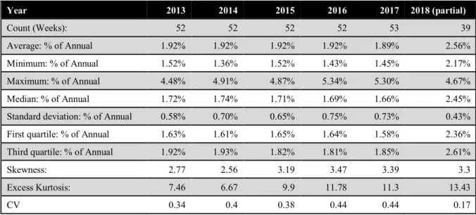
The consumption data of King’s Hawaiian bread are reported separately from that of other King’s Hawaiian food categories, and therefore are already restricted to the relevant products and aligned with the filtered shipment data set. Consumption statistics were evaluated as the total number of units sold, regardless of region, for each week beginning in 2013 through period 9 of 2018. Table 3.5 presents the summary statistics for consumption. Consumption data used in the forecast included all of 2018.
Table 3.5 Summary Statistics for Consumption Actuals
Year 2013 2014 2015 2016 2017 2018 (partial) Count (Weeks): 52 52 52 52 53 39 Average: % of Annual 1.92% 1.92% 1.92% 1.92% 1.89% 2.56% Minimum: % of Annual 1.52% 1.36% 1.52% 1.43% 1.45% 2.17% Maximum: % of Annual 4.48% 4.91% 4.87% 5.34% 5.30% 4.67% Median: % of Annual 1.72% 1.74% 1.71% 1.69% 1.66% 2.45% Standard deviation: % of Annual 0.58% 0.70% 0.65% 0.75% 0.73% 0.43% First quartile: % of Annual 1.63% 1.61% 1.65% 1.64% 1.58% 2.36% Third quartile: % of Annual 1.92% 1.93% 1.82% 1.81% 1.85% 2.61%
Skewness: 2.77 2.56 3.19 3.47 3.39 3.3
Excess Kurtosis: 7.46 6.67 9.9 11.78 11.3 13.43
CV 0.34 0.4 0.38 0.44 0.44 0.17
As expected, due to the correlation between unit sales and shipments, a similar positive trend was detected in the annual consumption volume. Also similar is the large range between the minimum and maximum amount purchased. Unlike shipments, the minimum volume of units sold each year does not vary as significantly as the minimum pounds shipped. Additionally, the coefficient of variation for the consumption is lower than that of shipments, suggesting shipments are subject to the bullwhip effect.
3.2.2 Seasonality
It is well understood within King’s Hawaiian that their demand is highly seasonal. The primary season is centered on the US holiday Thanksgiving, with the Christmas holiday a close second in terms of the magnitude of sales. Easter also drives high sales, as do other key events such as championship football
23 games, and federal holidays such as Labor Day. Seasonality is mapped at King’s Hawaiian using a
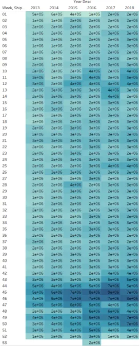
calendar that assigns a label, or seasonal identifier, to each week of the year. A heat map (Fig 3.4) helps identify the duration of the seasons, and whether there is a lag between the change in shipments and the known seasonal event. The seasonal labels uniquely identify the timeframe, lag, and duration for key recurring seasonal events that historically affected (both positively or negatively) shipments.
Fig 3.4 Heat Map of Total Shipments. Darker colors indicate higher volume of shipments and reveal
24
3.2.3 Severe Weather Data
Climate data in the form of severe weather events were gathered from NOAA using their Storm Events Database. Records of storm events were collected from 2013 through October 2018. Initial records included geographic areas, bodies of water and US territories that were excluded from the analysis which reduced the number of regions from 68 down to the 50 states. Storm events were recorded at the
resolution of daily events, which were then aggregated to the weekly level. Storm events cataloged range from dense fog to hurricanes, with a total of 56 unique categories. After excluding marine specific events and less severe categories, 17 categories of severe weather events remained for consideration. To quantify the severe weather events, the counts of unique events in each category were aggregated for each state, each week. To normalize the impact of typical weather patterns, the weather events were assigned a positive binary value only if the sum of the count of the specific weather events exceeded one standard deviation above the mean for the month for each state.
3.2.4 Census Data
Data were collected for all US States, Washington D.C., and Puerto Rico from 2013 to 2017. The data for these date ranges are estimates, unlike the physical counts obtained every ten years. 2018 data were not available. The inability to collect census data for the current year highlights a challenge of using publicly available data sets. To make use of the census data as a predictive indicator of demand, 2017 data were used as a proxy for 2018. This was judged this to be a safe assumption as the year-over-year variation within each category was not large, and typically fell within the census published margin of error. The imputation of the annual census data allows for the inclusion of 2018 data and is a key assumption made to align data sets with complementary data.
Since the approach was to use a random forest model to determine the appropriate combination of attributes for forecasting demand, the census data were restricted to only the primary attributes, ignoring attribute combinations and subsets. The census data required enhanced scrubbing to align timeframes. Not all attributes were consistently estimated each year, or else had slight differences in descriptions. To
25 ensure a complete data set, attributes were restricted to those that were present across the entire timeframe considered and matched descriptions. Attribute descriptions were then abbreviated and, in some cases, truncated to fit within database parameters. Table 3.6 shows the starting attributes and the result of multiple rounds of transformations.
Table 3.6 Census Data Attribute Summary
Classification Original Attributes Refined Attributes
Population 357 27
Education 769 15
Ethnicity 21 8
Household 201 22
Income 169 14
- Population data were collected from the US Census data set designated DP05. The population data set included attributes that were subsets or combinations of attributes. The data set was restricted to select only total population and age range percentages, by state.
- Education data were collected from US Census data set S1501. 2013-2014 data presented education ranges as percentages of the population within an age range. 2015-2017 data showed the count of the population within that age and education range as opposed to the percentage. To normalize the data, all attributes were converted to percentages of the population for that category age range.
- Ethnicity data were selected from the US Census data set B02001. Due to the potential combination of ethnic backgrounds, attributes were restricted to either single defined ethnic groups or a combination. To normalize the data by state, attributes were converted to percentages of the state population. Ethnicity data were unavailable for 2017 and 2018, so 2016 data were used as a proxy for both 2017 and 2018.
- Household data were selected from the US Census data set S1101. The data were filtered into primary categories and restricted subset combinations of attributes. Data were presented as
26 percentages of homes that fell within the primary category, or the mean percentage of homes that fell within the category.
- Income data were selected from the US Census data set S1902. The attribute median income, in US dollars, was selected as the primary measure.
3.3 Data Pre-Processing
Integrating multiple data sources required significant levels of pre-processing and secondary
transformations to ensure alignment and relevancy. This section discusses the process of aligning multiple data sources.
3.3.1 Aggregation
To capture the unique perspectives of the external data sources that can be leveraged by machine learning forecast models, an appropriate level of resolution was required. Shipment data are available down to the city, state level. Data are based on the customer ship to location, which is typically a large DC that feeds multiple different stores in different cities. Consumption is similarly discrete, reflecting sell-through data at the city level. However, like shipments, these data are often the aggregated consumption for the wider metropolitan area. King’s Hawaiian’s 3PL network generally aligns to geographic regions such as North East, and Midwest, with each 3PL supplying product for multiple states.
For demand forecasting, the level of aggregation selected was the state resolution. Aggregation to the state level allows for the use of both internal shipment data and external data sets such as consumption, with a higher degree of confidence that they are reflective of the broader area. Additional data sources such as socio-economic census data and weather data must be aggregated to the same resolution.
King’s Hawaiian’s current demand forecasting methodology is at the weekly level. To align the proposed machine learning forecast as much as possible, the data were aggregated to the resolution of a week. King’s Hawaiian shipment data and weather data were the two data sets that had a temporal resolution down to the day and had to be aggregated to weekly. Shipments were aggregated by summing the daily sales within that week. For climate data, the counts of severe weather events one standard deviation above
27 the mean that occurred each week were used. Consumption data as currently purchased is already set at the weekly resolution and therefore will require no aggregation. Census data are annual and were therefore disaggregated to the weekly level. As a simplifying assumption, weekly census data was assumed to mirror that of the annual data for each year.
3.3.2 De-Seasonalizing
Demand was de-seasonalized to improve the predictive performance of the machine learning models. Machine learning models can be overly influenced by strong seasonal patterns, ignoring other important patterns and trends due to the magnitude of variation caused by seasonal factors. For regression models in general, de-seasonalizing the data is expected to improve the fit and predictive power of the model.
3.3.2.1 Shipments
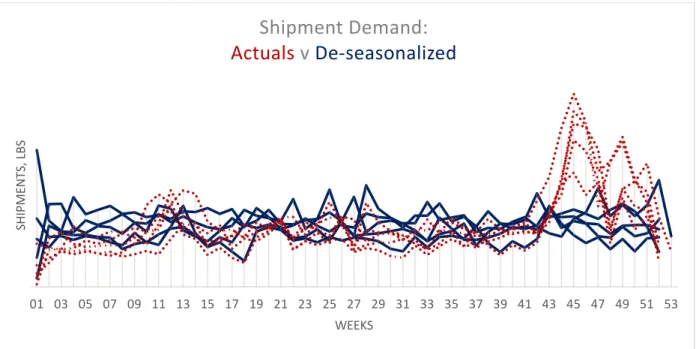
Visualization of the actual shipment demand (Fig. 3.5) confirmed the presence of a strong seasonal element.
Fig 3.5 Shipments, De-seasonalized. Weekly total brand shipment data shown in both seasonal (red
dotted lines) and de-seasonalized (solid blue) for multiple historic years
01 03 05 07 09 11 13 15 17 19 21 23 25 27 29 31 33 35 37 39 41 43 45 47 49 51 53 SH IP M EN TS, L BS WEEKS
Shipment Demand:
Actuals
v
De-seasonalized
28 Magnitudes were calculated by taking the quotient of actual shipments and the annual mean on a per SKU, per year basis. The mean seasonal magnitude was then calculated for each seasonal identifier. Shipments were de-seasonalized using the company assigned seasonal identifiers and the mean SKU specific magnitudes.
Outliers such as the first week of 2017 can generate variation as significant as normal seasonality, even after the shipments have been normalized. This event, while believed to be replenishment from an
unexpectedly large sell-through effort due to a single large retailers’ aggressive merchandising, highlights the volatility in shipments and the outsized impact a single retailer can have on demand.
3.3.2.2 Consumption
Visualization of the consumption demand (Figure 3.6) aligned with, and demonstrated an even more distinct seasonality than, the shipment data.
Fig. 3.6 Consumption, De-seasonalized. Weekly total brand consumption data shown in both seasonal
(red dotted lines) and de-seasonalized (solid blue) for multiple historic years
01 03 05 07 09 11 13 15 17 19 21 23 25 27 29 31 33 35 37 39 41 43 45 47 49 51 53 CO N SU M PT IO N , U N IT S WEEK
Consumption
Actuals
v.
DeSeasonalized
29 Consumption was de-seasonalized using the company assigned seasonal identifiers. Seasonal magnitudes were calculated by taking the quotient of actual consumption and the annual mean on a total unit basis. The mean magnitudes were then calculated across 2013-2017 for each seasonal identifier.
Outliers such as week 46 consumption demand, which was likely caused by an aggressive merchandising effort at a large retailer, demonstrates how sensitive consumption demand signals can be to specific actions at the retail level.
3.3.3 Aligning by State
The data were aggregated to the state level because this resolution allowed for the best alignment of the data sets with the highest degree of confidence. While nearly all of the data sets cover all 50 states, the shipment data available from King’s Hawaiian show that from 2013 through 2018, they had not shipped to all 50 states. Since the target of the forecast is shipments, external data sets were aligned to the resolution of the shipment data.
3.3.4 External Attribute Incorporation
External data were incorporated into the analysis by joining data sets on two different attributes. The first attribute was regionality, set to the resolution of state. The second attribute was a temporal variable with data joined by year and week number. Additionally, consumption data were joined on the product attribute. External data sets were joined in SQL to improve the speed of analysis, as well as allow for analysis on the characteristics of the individual data sets.
3.3.5 Data Partitioning
The data were partitioned into two sections for training and testing. The models were trained on data from 2013 through 2017. The models were then tested against actuals from 2018. Each model also underwent a three-fold cross-validation to improve understanding of the accuracy of the model and reduce the
30 The King’s Hawaiian statistical model was trained on data beginning in 2012 and undergoes a monthly update as part of the ongoing S&OP process. It was this S&OP updated 2018 statistical forecast that was evaluated against the machine learning forecast.
3.4 Data Scrubbing
Data were preprocessed and joined into a unified data set in SQL. After data were pre-processed in SQL, it underwent a scrubbing process in Python prior to input into the models. Data were randomly sampled and visualized for each of the data scrubbing steps, and summary statistics generated, to ensure the data cleansing process was effective and data integrity was not compromised.
3.4.1 Temporal Alignment
To ensure comparable availability of data for demand forecasting in practical use, shipment data (the target of the demand forecast) was offset by one week to all other associated data. This lag of one fiscal week ensured that the predicted value for the shipment demand was based on consumption and weather events from the preceding week and that the model would not have visibility to the current week’s shipment performance for use in its predictions.
3.4.2 Product Specific
SKU specific shipment data was not consistently available for every product for the complete timeframe being evaluated. To align data and account for the updated products and limited time promotional offerings, all products were classified based on their fundamental selling unit. Since demand was being evaluated in pounds of product, this eliminated any issue of variable secondary or tertiary packaging configurations.
Not all products had historical data back through 2013, such as newer products for club store channels. Due to the nature of machine learning algorithms, gaps or holes in data can significantly skew the results. Since newer products did not always have a comparable analog in the historical data or could not be accurately segregated from the historical data to prevent double counting the demand, any SKU without a
31 complete historical data set was dropped from the analysis. This reduced the product count down to 10 final SKUs.
The shipment demand for the remaining 10 SKUs was visualized through Tableau to confirm the consistency of shipments at the national level. SKUs that had gaps identified were investigated as to the underlying cause. If the demand was found to be missing as a result of non-market driven forces, such as manufacturing disruption causing inventory stock outs, then those records were also dropped from the analysis.
3.4.3 Regionality
Regional data labels were standardized to two characters and any out of scope region was dropped from the data set. While census, weather and consumption data were available for every state, shipment data were not. This is because not every state has King’s Hawaiian product sold directly to an entity in each state, as certain customers and regions are supported by out of state distribution centers or distributors.
3.4.4 Weather
Weather data were not available for the final two months of the 2018 test data set. This timeframe was included in the evaluation absent this data as it represents a real limitation of using publicly available data for forecasting.
Weather data were also engineered into three new binary attributes; summer, winter, and high damage. If the occurrence for any of the underlying weather types were identified as having occurred per the
selection criteria described in section 3.2.3, then the new attributes indicated the occurrence.
3.4.5 Census
Census attributes that evaluated the same underlying data in different subsets were restricted to a single set that was mutually exclusive and collectively exhaustive. Categories that exhaustively covered a characteristic were broken down into two or more complementary attributes. Census data is often reported as a percentage of the population for the geography; however, the unit of measure was not consistently
32 represented in the data. All census data that were reported in percentages were normalized to range from zero to one. Attributes categories that had data represented as both a percentage as well as the numerical counts of populations were restricted to the percentages only when possible.
3.4.6 Data Cleansing
The data set was scrubbed of any outliers or duplicates. Duplicated records were dropped after data aggregation had been performed. Records that contained multiple nulls or negative values for any of the attributes were removed. A small number of missing records with missing data were imputed with the mean of the attribute for the class within that feature. Negative values for shipments were extremely limited, and an artifact of an inventory reconciliation mechanism for accounting purposes.
3.5 Data Normalization
To ensure optimum results from the machine learning algorithms and to minimize the impact of dissimilar data scales, all data were normalized prior to forecasting. Categorical values were converted to binary representations via one-hot encoding to improve the effectiveness of the predictions. Census data reported as percentages were normalized to ranges between zero and one. Weather data and the engineered
weather category attributes were converted to binaries as part of pre-processing. Non-range bound data such as shipment and consumption data, as well as population totals, were standardized by removing the mean from each value and dividing by the standard deviation as part of the transformation pipeline processing. These transformations were calculated from the training set only, with the values being applied to the test set for final verification.
3.6 Feature Selection and Engineering
One important advantage of using machine learning models versus traditional methods in demand forecasting is the ability to perform analysis using not just the internal demand data but also incorporate data from different, external sources. By doing so, demand planners can answer a broad range of questions (e.g. what is the impact of weather events on demand?). However, answering those questions
33 requires including more features in the model and as more features are added the model becomes more complicated, potentially overfitting and running slower. Therefore, feature selection is an important step in building models. For this project, multiple feature sets were evaluated, using different evaluation criteria.
The Feature Select 1 set employed a random forest model, a type of ensemble machine learning technique that is frequently used in feature selection, to identify attributes that have an assigned importance rating above a set threshold of 0.1%. Random forests are described in section 3.7, along with other machine learning models, as the same technique will also be used in developing forecasting models.
Feature Select 2 set was also created using the consumption and census features from Feature Select 1, but replaced storm events with the engineered weather feature attributes discussed in section 3.4.4.
3.7 Machine Learning Models
A large number of machine learning models can be applied in demand forecasting. Five models were selected that were considered to be most suitable for the task based on the literature review. Based on the research, random forests, artificial neural networks, support vector machines, gradient boosting, and k-nearest neighbors have a high potential in decreasing demand forecasting error. A three-dimensional cube search was performed of those models by varying different hyper-parameters (e.g. different number of layers in artificial neural network models) and using different features (e.g. seasonal vs de-seasonalized target data) to compare the performance of the different models.
3.7.1 Random Forests (RF)
Random forests are a type of ensemble methods where multiple decision trees are used for classification or regression. The goal is to decrease the variance by combining trees built using random samples of the data and random subsets of features. Decision trees are built by separating the data at nodes using an algorithm that determines the best split. Multiple algorithms can be used to construct a decision tree. Random forest is an ensemble machine learning approach since it combines multiple different trees when evaluating the best fit.
34 Random forests are powerful enough to model complex nonlinear relationships. On the other hand, their outputs are not easily interpretable as they come from a combination of multiple trees.
3.7.2 Artificial Neural Networks (MLP)
Artificial neural networks are inspired by how neurons and synapses in the brain work and they can be used to model complex relationships. Neural networks consist of nodes that are used to calculate the weights of the features in the model. The inputs to each node are outputs of the nodes in the previous layer and their associated weights. The output of a node is calculated by evaluating an activation function using the weighted average of the previous layers’ outputs. The nodes are organized in layers and as the number of layers increases, the neural network is considered to become a deep neural network.
Depending on the number of nodes, the layer structure and the algorithms used, neural networks can take many different forms. The most commonly used type of neural networks called multilayer perceptron (MLP) were used.
Multilayer perceptron models are feed forward neural networks where the information flows in one direction, i.e. from the input layer to the output layers. An arbitrary number of hidden layers can exist between the input and output layers. A multilayer perceptron with one hidden layer can approximate any continuous function. The network can be trained using a backpropagation algorithm.
3.7.3 Support Vector Machines (SVR)
Support vector machines (SVM) are used in tasks like classification and regression. They employ a decision boundary called a hyperplane. The approach is to maximize the minimum margin, i.e. the distance between the hyperplane and the nearest data point.
Support vector machines can model non-linear relationships using a kernel method, which maps the data points that have a non-linear boundary to a higher dimensional space where it is easier to separate them. Polynomial and Gaussian are two of common kernels. SVMs can be slow to run and the outputs can be difficult to interpret.
35
3.7.4 Gradient Boosting (GB)
The goal of boosting methods is achieving better results by combining weaker models. There are many boosting models like adaboost and gradient boosting. They can be used for both classification and regression tasks.
Gradient boosting is an ensemble method where predictors are added sequentially. In each stage, the new predictor is fit into the residual errors. The new predictors are regression trees in the gradient boosting regression model that was used from the scikit-learn library.
3.7.5 K-Nearest Neighbors (KNN)
K-nearest neighbors is a model that can be used for both classification and regression. Its intuitiveness and ease of implementation made KNN a popular tool among practitioners, especially for classification tasks. In classification, the class of an observation is determined by a vote of the k number of neighbors closest to the observation based on a distance metric. Similarly, in regression tasks, the value of the target is determined by taking an average of the k closest observations.
KNN models are generally fast to train as they do not need to take all the data into consideration, they evaluate the value of the targets based on only k observations. The optimal value of k is generally determined by running the model with different k values and comparing the results.
3.8 Performance Measurement 3.8.1 Forecast Error
King’s Hawaiian’s current statistical Holt-Winters forecast performance is calculated at two different levels. The first level is the total network forecast or the performance for the SKU across the sum of all selling regions. The forecast error is calculated as the absolute percent error, weighted by forecasted demand for each SKU (WAPE). While the forecast is generated at a week level, the current forecast error is calculated monthly for inventory policy purposes (Fig 3.7).
36 Fig 3.7 Current Network Level Forecast Performance. Forecast error (WAPE) by period for all core
bread SKUs at the network level
The performance of this regional forecast is evaluated similarly to the network forecast (Fig 3.8), using the weighted absolute percent error (WAPE).
Fig 3.8 Current Statistical Forecast Regional Forecast Performance. Weighted absolute percent error by
period by region when aggregated to King’s Hawaiian distribution regions
The regional forecast has achieved a mean monthly forecast error of ~34% in 2018. This is a significant change in the accuracy of the regional forecast, which improved dramatically from 2017 to 2018 as a result of the implementation of an improved methodology for the calculation of the regional distribution