Modelling Data Processing for Interactive Scores Using Coloured Petri Nets

(1)

HAL Id: hal-01095176

https://hal.archives-ouvertes.fr/hal-01095176

Submitted on 22 Sep 2015

HAL is a multi-disciplinary open access

archive for the deposit and dissemination of

sci-entific research documents, whether they are

pub-lished or not. The documents may come from

teaching and research institutions in France or

abroad, or from public or private research centers.

L’archive ouverte pluridisciplinaire HAL, est

destinée au dépôt et à la diffusion de documents

scientifiques de niveau recherche, publiés ou non,

émanant des établissements d’enseignement et de

recherche français ou étrangers, des laboratoires

publics ou privés.

Modelling Data Processing for Interactive Scores Using

Coloured Petri Nets

Jaime Arias, Myriam Desainte-Catherine, Camilo Rueda

To cite this version:

Jaime Arias, Myriam Desainte-Catherine, Camilo Rueda. Modelling Data Processing for Interactive

Scores Using Coloured Petri Nets. 14th International Conference on Application of Concurrency to

System Design, Jun 2014, Tunis, Tunisia. �10.1109/ACSD.2014.23�. �hal-01095176�

(2)

Modelling Data Processing for Interactive Scores

Using Coloured Petri Nets

Jaime Arias, Myriam Desainte-Catherine

Univ. Bordeaux, LaBRI, Bordeaux, F-33000, France CNRS, UMR 5800, Bordeaux, F-33000, France

IPB, LaBRI, Bordeaux, F-33000, France Email: {jaime.arias, myriam}@labri.fr

Camilo Rueda

Departamento de Electr´onica y Ciencias de la Computaci´on Pontificia Universidad Javeriana

Cali, Colombia

Email: crueda@javerianacali.edu.co Abstract—I-score is a system for the composition and

ex-ecution of interactive multimedia scores. It uses Hierarchical Time Stream Petri Nets (HTSPN) to build an execution model of the scores. Nowadays, composers have increasingly needed to represent and manipulate complex data in their multimedia scenarios. However, HTSPN formalism does not allow to handle data. In this work, we propose a model to execute interactive multimedia scores based on Coloured Petri Nets (CPN). Our work extends the current execution model of i-score with the capability to handle complex data. Our approach consists in developing CPN modules for reading, appending and reversing audio files. We use CPN Tools for prototyping, simulating and verifying our model and discuss how to represent fundamental signal processing functions, conditionals or loops.

Keywords—coloured petri nets; data processing; formal speci-fication; interactive scores;

I. INTRODUCTION

Nowadays, the design of interactive multimedia systems based on a written scenario is a challenge that requires to handle dynamic and static events as well as dynamic and static data. Interactive scores [1] propose a model to write and execute interactive scenarios comprised of several multimedia processes. This model provides a real-time control of the dynamic and static events, and also it preserves the temporal organization of the scenario during the writing and execution stage.

I-SCORE[2] is a software that allows to design and execute

interactive and multimedia scenarios. The execution model is based on Hierarchical Time Stream Petri Nets (HTSPNs) [3]. Places and transitions of Petri nets model temporal aspects of the scenario (i.e., they define a partial order between static and dynamic events) defined during its composition.

This paper presents an extension of I-SCORE that aims to

handle: (1) complex data, in particular, dynamic and static data streams; and (2) dynamic and static events. The extension adds the possibility of building stream processing structures by functional composition of processes through input/output data slots. Our main idea is to use Coloured Petri Nets (CPNs) [4] to model complex data and the dynamic aspect of the functional composition of processes. Multimedia streams are often cut into temporal frames to be carried from one process to another. Then, in our approach, we model frames as coloured tokens that are handled by processes.

The extension we propose provides the notion of asyn-chronous functional composition. This corresponds to the case where the composed processes are not executed at the same time. Then, it requires to buffer the output data stream of processes in order to hold data until another process read them. In the context of interactive scores, the date in which the buffers will be read may not be known at composition nor execution time. Nevertheless, the duration of the buffers are all bounded by the duration of the scenario which is finite. Therefore, we are very interested in verifying properties of scenarios by using the verification methods of CPNs.

The rest of the paper is organized as follows. In Section II

we briefly present the I-SCORE system and the Coloured

Petri Nets formalism. In Section III we develop a model for executing interactive scores using Coloured Petri Nets. In Section IV, we extend our model for handling complex data. Finally, in Section V we present conclusions, and future work.

II. PRELIMINARIES

In this section we first briefly present theI-SCOREsystem.

Then, we present the basic notions of Coloured Petri Nets (CPNs), and we also show a tool for editing, simulating and verifying CPNs models.

A. I-score

I-SCORE is a software for the composition and execution of interactive multimedia scores [1], [2]. It consists of two sides: authoring side and performance side. The authoring side allows the composer to design a scenario. On the other hand, the performance side executes the scenario in real-time with interactive capabilities.

1) Authoring side: In this side the composer designs a

scenario as a collection of multimedia objects that are rep-resented as boxes on a sheet in which the horizontal axis represents the time-line and the vertical axis has no meaning. The boxes are temporal structures with a start date, a duration

and a multimedia process. In I-SCORE, the execution of the

multimedia processes is carried out by external applications

such as MAX/MSP1 _{or P}_URE_D_ATA2_{, and it uses multimedia}

protocols such as OSC3 _{to send values/parameters to them.}

1_{http://cycling74.com/products/max/} 2_{http://puredata.info}

(3)

The composer can use hierarchical boxes for grouping several boxes with their own temporal organization. Hierarchical boxes eases the design of large scenarios. In fact, the whole scenario is represented as a hierarchical box.

The composer partially defines the temporal organization of the scenario using Allen temporal relations [5] between the boxes. These represent temporal precedences between boxes, that are complemented with quantitative measures in the form of durations. It is possible thus to express that the start of some box must be separated from the end of some other by a

given duration. I-SCORE allows composers to build interactive

scores adding discrete interactive events which are triggered in execution time and modify either the start date or the duration of the boxes. It is important to note that temporal relations are preserved during the authoring and performance sides. For this reason, a scenario can be interpreted in a limited set of possibilities.

In Figure 1, we show an interactive scenario where: the box A has no interaction points, then it has a fixed start date and duration; the box C has an interaction point at the start, then the start date can be modified in execution time; the box D has an interaction point at the end, then the duration of the box can be modified in execution time; and the box B combines the two above behaviours. Note that the temporal relations preceding the boxes B and C are represented as dashed arrows, it means that the duration of the temporal relation is partially defined by a range of possible values. Otherwise, the duration of the interval is fixed and it is represented as solid arrows.

max C D A Bmax min time max min min min r1 r2 r3 r4 r5 r6

Fig. 1. Example of an interactive scenario.

2) Performance side: I-SCORE translates the scenario into

a Hierarchical Time Stream Petri Net (HTSPN) [3] structure for its execution. The equivalent HTSPN structure allows to trigger interactive events, and also preserves the temporal organization during the execution of the score. The method for transforming a score into a HTSPN structure is described as follows [2].

• Turn into transitions each control point (i.e., the start

and the end of the boxes).

• Merge the transitions that represent control points that

are executed at the same time.

• Add a sequence arc/place/arc between two transitions

that have a temporal relation. Add the duration of the relation on the arc.

• The crossing condition of the transitions that represent

control points with an interaction point is conditioned by receiving an external message. Moreover, the tran-sition is fired automatically if the external event is not triggered between the interval of time specified by the composer.

Following the above steps, we translated the scenario shown in Figure 1 into its equivalent HTSPN structure (Fig-ure 2). Here, the transitions with double stroke represent interaction points and the labels on the arcs define the duration of the relation. As mentioned above, the scenario is represented as a hierarchical box, then the relations r1 and r2 begin from the start of the scenario (i.e., transition S(S)). Additionally, the end of the scenario (i.e., transition E(S)) is defined by its duration (i.e., relation r9), and the end of the boxes C and D.

S(S) S(A) E(S) E(A) S(B) E(B) S(C) E(C) S(D) event()E(D) event() event() event() r1 r2 r3 r4 r5 r6 r7 r8 rA rB rC rD r9

Fig. 2. HTSPN structure of the scenario shown in Figure 1.

B. Coloured Petri Nets

Coloured Petri Nets (CPNs) [4] is a graphical language for modelling and verifying concurrent and distributed systems. It combines the well-defined Petri Net model with the power of the high-level programming language, Standard ML.

CPN models can be simulated, then it allows to explore the possible behaviours of the system. In addition, CPN supports hierarchical composition which allows to structure a model into a set of modules. This feature is very important to model large systems. Another advantage of CPNs is the capability to express the notion of time. Next, we present the definition of Coloured Petri Net [4].

Definition 1: A timed non-hierarchical Coloured Petri Net

is a nine-tuple CP NT = (P, T, A, Σ, V, C, G, E, I) where:

1) P is a finite set of places.

2) T is a finite set of transitions such that P ∩ T = ∅.

3) A ⊆ P × T ∪ T × P is a set of directed arcs.

4) Σ is a finite set of non-empty colour sets. Each colour

set is either untimed or timed.

5) V is a finite set of typed variables such that

T ype[v] ∈ Σ for all variables v ∈ V .

6) C : P → Σ is a colour set function that assigns a

colour set to each place. A place p is timed if C(p) is timed, otherwise p is untimed.

7) G : T → EXP RV is a guard function that assigns

a guard to each transition t such that T ype[G(t)] = Bool.

8) E : A → EXP RV is an arc expression function that

assigns an arc expression to each arc a such that

(4)

• T ype[E(a)] = C(p)T M S if p if timed.

Here, p is the place connected to the arc a.

9) I : P → EXP R∅ is an initialisation function that

assigns an initialisation expression to each place p such that

• T ype[I(p)] = C(p)M S if p is untimed;

• T ype[I(p)] = C(p)T M S if p is timed.

The verification of CPN models is automatic and supported by the state space method. Roughly, this method computes all reachable states and state changes of the CPN model and represents them as a directed graph. In this graph, nodes represent states and arcs represent occurring events. From the state space, it is possible to verify some properties of the system such as absence of deadlock.

CPN TOOLS4is a tool for editing, simulating and analysing

CPNs models. This tool supports untimed and timed hierarchi-cal CPN models. Therefore, we can build large and modular models. The user works directly with the graphical represen-tation of the CPN model and the simulation can be carried out step by step or selecting the number of steps that will be exe-cuted. Also, we can define stop criteria and breakpoints. CPN

TOOLS can generate full state space to verify models, and it uses advanced methods to mitigate the state explosion problem. This tool also supports model checking. An interesting feature is the generation of sophisticated reports from the states of the

net during the simulation. Additionally, CPN TOOLS includes

a collection of libraries for various purposes. One example is

COMMS/CPN [6] that allows TCP/IP communication between

CPN models and external applications.

III. A MODEL FORINTERACTIVESCORES

In this section we present a model for executing interactive scores [7] using Coloured Petri Nets (CPNs) [4]. This model

allows to execute any scenario built in I-SCORE5.

As we explained before, in I-SCORE composers design a

scenario defining a partial temporal organization of multimedia elements, represented as boxes, by using temporal relations. Additionally, composers can add interaction points to modify either the start date or the duration of the boxes during the execution. The temporal relations must maintain during the

editing and execution time. Moreover, I-SCORE allows to

group boxes in a hierarchical box. This is very important for designing large scenarios.

In our approach we develop a CPN model for each structure that defines an interactive score (i.e, temporal relations, boxes and interaction points). This allows to build a modular and parametrizable model which can be reusable and extensible. In the following we present the implemented CPNs modules. A. Intervals

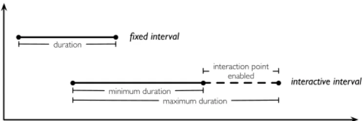
We model all elements of a score as intervals. These are classified into two classes: fixed intervals, and interactive

intervals(Figure 3). Fixed intervals are temporal relations with

a fixed duration, whereas interactive intervals have a range of values that define a minimum and a maximum duration.

4_{http://cpntools.org} 5_{http://i-score.org/}

Additionally, interactive intervals have attached an interaction point that stops the interval if it is triggered between the duration of the interval. We shall model boxes and interaction points from these two intervals.

time fixed interval interactive interval duration minimum duration maximum duration interaction point enabled

Fig. 3. Fixed and interactive intervals.

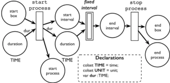
1) Fixed interval: A fixed interval consists in applying a

delay between two points. This delay can be implemented in CPN using the delay expression @+duration in the inscription of an output arc from a transition. As can be seen in Figure 4, if there is a token in the place start and a coloured token d in the place duration, they will be consumed by the transition and a token will be produced in the place end after d time units.

Declarations colset TIME = time;

colset UNIT = unit;

colset UT = UNIT timed;

var dur : TIME;

start duration TIME ()@+dur dur wait UT end ()

Fig. 4. CPN model of a fixed interval.

2) Interactive interval: An interactive interval applies a

delay between two points whose duration is flexible (i.e., it has a minimum and a maximum duration). The interval finishes when either it reaches the maximum duration or the attached interaction point is triggered after the minimum duration. Therefore, we decompose an interactive interval into a module for modelling the flexible duration and other for handling the interaction point.

We use two fixed intervals for modelling flexible intervals. The first interval waits for the minimum duration of the flexible interval, and the second waits for the remaining time of the maximum duration (Figure 5). Then, once the minimum interval finishes, the second fixed interval starts and waits for the remaining time. We handle an interaction point using a net that accepts an event if it is both triggered after the start of the module and before that a stop signal, otherwise it is ignored (Figure 6). The module finishes if there is an accepted event or a stop signal. We use the guards of transitions in order to ignore the events (i.e., consume the tokens) that were not triggered in the current time. An inhibitor arc removes the conflict generated when there is a stop signal and an event at the same time.

(5)

var dmin : TIME;

var dmax : TIME;

start interval _end interval 1 duration 1 TIME start interval 2 end max. interval duration 2 TIME dmin dmax-dmin dmin dmax end min. interval min. duration TIME max. duration TIME fixed interval fixed interval

Fig. 5. CPN model of a flexible interval.

colset UT = UNIT timed;

var ip_t : TIME;

start stop end interact. point enabled ip_t ip_t TIME UT t3 ()@+1 time() t1 [ip_t < time()] t2 [ip_t = time()]

Fig. 6. CPN model for handling an interaction point.

Now, we use the above two modules to model interac-tive intervals (Figure 7). Therefore, we start the module for handling interaction points when the minimum duration is elapsed and we stop it when the flexible interval reaches the maximum duration. We limit the number of times that the module can be stopped (place “enable”) if there are several intervals sharing the same interaction point. We shall discuss this in Subsection III-D.

B. Boxes

In I-SCORE, multimedia elements are temporal structures

represented as boxes. A box has a duration and a start date which can be modified in the execution time by adding interaction points. The temporal properties of the scenario must be maintained during the edition and execution time. In our approach, we model boxes as fixed or interactive intervals with an attached process. Our models of the different cases of boxes are described below.

1) Fixed box: A fixed box is modelled as a fixed interval

with a specific duration. In addition, the attached process starts

colset BOOL = bool;

var e : BOOL; interact. point start get stop get end interval get IP ss se flexible interval start interval TIME max. duration TIME min. duration end max. interval end min. interval enable e false BOOL true if (e=true) then 1`() else empty

Fig. 7. CPN model of an interactive interval.

and finishes with the interval (Figure 8). We represent these events as transitions. start box start process end box stop process dur dur duration TIME start process start interval end interval fixed interval duration TIME end process Declarations

colset TIME = time;

var dur : TIME;

Fig. 8. CPN model of a fixed box.

2) Interaction point at the start of the box: An interaction

point at the start of the box allows to anticipate or delay the

start of the box during the execution. In I-SCORE, composers

define an interval of time in which a specific event can be trig-gered. Then, the box will start if the event is triggered during the interval or the interval reaches its maximum duration. In our approach, we model this box adding an interactive interval at the start of a fixed box that controls the beginning of the box because it has attached an interaction point (Figure 9).

TIME duration start box start process end process end box fixed box TIME max. duration start interval TIME min. duration interact. point end interval interactive interval Declarations colset TIME = time;

(6)

3) Interaction point at the end of the box: The duration of a box can be modified during execution if it has an interaction point at the end. Composers define an interval of time in which a particular event can be triggered. Then, the box will finish if the event is triggered during the interval or the box reaches its maximum duration. We model this box replacing the fixed interval of the fixed box (see Figure 8) with an interactive interval (Figure 10). The interactive interval handles the interaction point of the box and constraints the duration of the box.

var dmin : TIME;

var dmax : TIME;

start box start process end box dmin min. duration TIME start process end process stop process TIME max. duration start interval TIME min. duration interact. point end interval interactive interval max. duration TIME dmax dmin dmax

Fig. 10. CPN model of a box with an interaction point at the end.

4) Interaction point at the start and at the end of the box: InI-SCORE, composers can combine the two above behaviours. We take advantage of the modularity of our approach for modelling this box. Then, we only need to add an interactive interval before the start of a box with an interaction point at the end (Figure 11).

start process TIME max. duration 2 TIME min. duration 2 start box end process end box interact. point 2 box ip end TIME max. duration 1 start interval TIME min. duration 1 interact. point 1 end interval interactive interval

Fig. 11. CPN model of a box with an interaction point at the start and at the end.

C. Hierarchy

Hierarchy is very important for building complex scenarios.

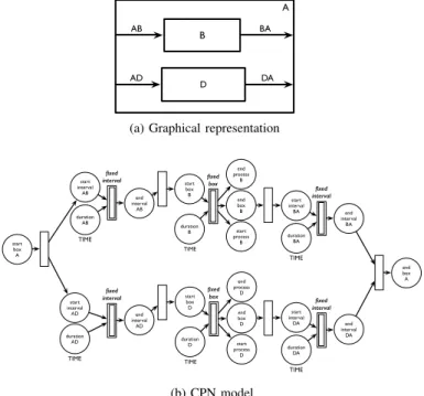
I-SCORE supports this feature allowing to group boxes in a hierarchical box. Indeed, the scenario is represented as a hierarchical box which contains all boxes, hierarchical boxes, temporal relations and interaction points. In our approach, a hierarchical box consists of two transitions for synchronizing the start and the end of its children. Furthermore, its duration depends on the temporal organization of the sub-scenario. We illustrate our idea in Figure 12.

Note that relations AB and AD start from the transition that represents the start of the hierarchical box. Then, these

B

A

AB BA

D

AD DA

(a) Graphical representation

TIME duration D start box D start process D end process D end box D fixed box TIME duration B start box B start process B end process B end box B fixed box start interval AB end interval AB duration AB TIME fixed interval start interval BA end interval BA duration BA TIME fixed interval start box A start interval AD end interval AD duration AD TIME fixed interval start interval DA end interval DA duration DA TIME fixed interval end box A (b) CPN model

Fig. 12. Example of a hierarchical box with two children.

relations will start at the same time that box A. Moreover, observe that there is an arc between the end of the relations

BA and DA, and the transition that represents the end of the

hierarchical box. Therefore, the hierarchical box A will end when all the above relations finish.

In this paper, we only consider interaction points at the start of hierarchical boxes in order to simplify the presentation of the model. Interaction points at the end involve executing complex mechanisms to stop recursively the children of boxes. D. Synchronization

Temporal relations define the beginning of boxes. There-fore, a box starts when all its preceding relations are satisfied. In I-SCORE, all relations preceding a box are flexible if the box has an interaction point at the start. Otherwise, they are fixed. In the following we introduce a merging operation to reduce several relations of the same type into an equivalent interval. The above allows to create a generic mechanism for maintaining the temporal relations in our model.

1) Merging fixed intervals: The fixed relations preceding a

box must be fulfilled. Then, the box will start when all fixed intervals finish. We illustrate the above behaviour in Figure 13 that is the time-line of an execution of the scenario shown in Figure 1. In this scenario, the box D has two preceding relations with fixed durations. Therefore, as can be seen in Figure 13, this box starts when the last interval finishes (i.e., interval r6 at 16 seconds).

In our model, we merge several fixed intervals synchro-nizing their ends with the start of a box by using a transition (Figure 14). Then, the box will start when all its preceding relations have finished.

2) Merging interactive intervals: Temporal relations

pre-ceding a box with an interaction point are flexible (i.e., they have a minimum and a maximum duration). In that

(7)

C A time (s) 0 1 2 3 4 5 6 7 8 9 10 11 12 13 14 15 16 17 r1 18 min max r2 B min max min max r3 r5 r6 19 20 21 22 23 D min max r4 min max

Fig. 13. Time-line of an execution of the scenario shown in Figure 1.

end interval r5 fixed interval end interval r6 fixed interval TIME duration box D start box D fixed box

Fig. 14. CPN model for synchronizing fixed intervals.

case, the box will start when one of its preceding relations reaches its maximum duration or the event attached to the box is triggered after all relations have reached their minimum duration (Figure 15). interactive interval 1 interactive interval 2 merge interactive (1,2) min max min max min max interaction point enabled time

Fig. 15. Merging two interactive intervals.

We illustrate the above behaviour in Figure 16 that shows an execution of the scenario in Figure 1. In this scenario, box C has two preceding relations with flexible durations. Therefore, the box may start during the flexible interval generated by merging the relations r3 and r4. As can be seen in Figure 16, the box C started at 9 seconds because an event was triggered during the interval merge(r3,r4). This interval represents the merging of the preceding intervals of the box, and it is defined by the minimum duration of the interval r4 and the maximum duration of the interval r3.

In our approach, we use interactive intervals to model temporal relations preceding a box with an interaction point. In order to merge several interactive intervals (Figure 17), we first split them into their two modules: flexible interval and interaction point (see Section III-A2). Then, we use a transition to synchronize the end of the minimum durations of all flexible intervals with the start of a module for handling the interaction point. Additionally, we connect the end of their maximum durations with the stop of the interaction point. As can be

C A time (s) 0 1 2 3 4 5 6 7 8 9 10 11 12 13 14 15 16 17 r1 18 min max r2 min max min max r3 r5 r6 19 20 21 min max r4 min max B D max min merge (r3,r4)

Fig. 16. Time-line of an execution of the scenario shown in Figure 2 with triggered interaction points. The symbol represents a triggered event.

seen in Figure 17, we limit the number of times the interval can be stopped by using the place enable and the transition se. TIME duration box C start box C fixed box end max. interval r3 end min. interval r3 flexible interval end max. interval r4 end min. interval r4 flexible interval get IP interact. point C start get stop get end get ss se enable e false BOOL true if (e=true) then 1`() else empty

Fig. 17. CPN model for synchronizing interactive intervals.

Hence, the box will start when an interval reaches its maximum duration or the event attached to the box is triggered after all its preceding relations have reached their minimum durations.

IV. ANEXTENSION FORHANDLINGCOMPLEXDATA

In this section, we present an extension of the model described in Section III for handling complex data. We take advantage of the coloured tokens of CPNs to represent audio streams. In our approach, an audio stream consists of a set of tokens whose colour is a tuple (i, d) where i is the index of the audio frame and d is its corresponding value. Additionally, the duration between each audio frame is preserved.

In the following we describe CPN modules for basic processing of audio files. First, we present a CPN model for reading audio files. Then, we show we can append and reverse files reusing the previous modules. Finally, we show the

(8)

A. Reading Audio Files

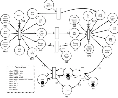
In our approach, reading audio files consists in acquiring audio frames from a file with a determined frequency (i.e., duration between frames). We show the model of the above behaviour in Figure 18. Here, the transition READ gets an audio frame (i.e., a coloured token) from the file each time the interval of time finishes. The transition will continue to read the frames until it reaches the end of the file (i.e., the maximum number of frames in the file) or there is a stop signal.

Observe that the inhibitor arc allows to solve the conflict generated when a stop signal is present at the same instant that a frame can be read. In addition, the place limit restricts the module to read a new frame only if the previous one was completely processed (i.e., the token is in the place output), and the place stop_enabled disables the stop transition when the module has finished.

The module has as output the read frames (place output) and the number of read frames (place frames_read). More-over, it also indicates if the module reached the end of the file (place EOF), and the instant when the interval of time between frames is elapsed (place next_frame). The last feature is useful if we want to synchronize the output of two files.

Declarations

colset INT = int;

colset BOOL = bool;

colset DATA = INT;

colset DURATION = TIME timed;

colset FILE = product INT*DATA;

var f_dur : TIME;

var e : BOOL;

var n_max : INT;

var n : INT; var f : DATA; TIME frame duration start INT max number frames f_dur n_max f_dur get frame DURATION f_dur f_dur@+f_dur max num INT n_max n_max n_max file FILE (n,f) continue stop next frame INT n+1 n receive frame FILE [n <= n_max] (n,f) (n,f) n_max n_max 1 if (n = n_max) then 1`() else empty (n,f) end EOF wait sync next frame f_dur R E A D limit if (n = n_max) then 1`() else empty if (e = true) then 1`() else empty 2`() n frames read n-1 INT stop enabled BOOL output FILE e 1`false e 1`false true

Fig. 18. CPN model for reading a file.

B. Appending Files

We append two files concatenating their outputs. We took advantage of the modularity of our model to build this module using the above. As can be seen in Figure 19, the module reads the first file, and once it finishes, it synchronizes the start of the reading of the second file. That means that the first frame of the second file will be read when the duration between the frames of the first file is elapsed (i.e., there is a token in the place next_frame).

Observe that the concatenated file is stored in the place output. We add an offset to the indices of the second file to correctly build the concatenated file (place index). Therefore, the outputs of the module are the appended file (place output) and the number of concatenated frames (place total_frames_read). The module will finish if both files are successfully read or there is a stop signal.

Declarations

var n : INT; var n1 : INT; var n2 : INT; var i : INT; var f : DATA; TIME frame duration file 1 start file 1 INT max number frames file 1 stop file 1 file 1 output file 1 FILE end file 1 EOF file 1 next frame file 1 TIME frame duration file 2 start file 2 INT max number frames file 2 stop file 2 file 2 output file 2 FILE end file 2 EOF file 2 next frame file 2 FILE FILE output FILE index (n,f) 1 INT i i+1 i i+1 (i,f) (n,f) (i,f) next 1 INT n n+1 next 2 1 INT n n+1 frames read 1 INT frames read 2 INT read

file readfile

total frames read INT n2 n1 n1+n2 stop append

Fig. 19. CPN model for appending files

C. Reversing Files

In our approach, the module reverses the order of a file in one instant of time, and then reads the output. As can be seen in Figure 20, we make use of the module for reading files to read the file in one time (i.e., the duration between frames is zero) while the transition REV reverses the order of its indices. Once the order of the whole file is inverse (i.e., the index of the reversed file is zero), another module starts to read the inverse file with a specific frequency. Observe that this module has the same outputs than the module for reading files.

Declarations

var n : INT;

var n_max : INT;

var i : INT; var f : DATA; TIME frame duration start reverse INT max frames stop file temp output FILE end EOF next frame TIME frame duration start INT max number stop reverse file reverse output reverse FILE end reverse EOF reverse next frame reverse FILE FILE (n,f) index INT i i-1 next 1 INT n n+1 0 INT max number frames [i=0] (i,f) [i>0] i n_max R E V n_max n_max n_max frames read INT frames reversed INT read

file readfile

(9)

D. Simulation

In the following we illustrate the use of the modules presented in this section by means of the scenario shown in Figure 21. Roughly speaking, the scenario first reads two files. Then, a box for reversing files receives, as input, the read frames of the second file to reverse them. Finally, a box for appending files receives, as input, the reversed file and the first file to concatenate them.

Append Files Read File 1 Read File 2 time (ms) max min min max Reverse File r1 (values) (values) (values) (param) (param) r2 r3 r4 r5

Fig. 21. Scenario with data processing.

As can be seen, the data processing modules are organized by using the elements described in Section III. For the sake of simplicity, we mixed boxes with processing modules in a single box. Additionally, we added to boxes inputs and outputs which are represented as points on each edge of the box. Intervals allow to communicate values between boxes and they are used as parameters of processes (e.g., number of frames, duration between frames). For example, the box for reversing files receives, as input, the output of the box for reading files through the interval r3.

Moreover, the duration of boxes can be constrained with the duration of their processes by adding an interaction point at the end of the box whose associated event is triggered when the process finishes. Observe that we use a different symbol in the box for appending files to represent the new interaction point.

Let us illustrate in Figure 22 a possible execution of the above scenario assuming the following configuration.

• The first file is composed of 4 frames, and each frame

must be played every 3 milliseconds.

• The second file is composed of 5 frames, and each

frame must be played every 3 milliseconds.

• Both files start to be read once the scenario begins.

• The reading of the first file must stop in 9

millisec-onds. However, it can be stopped by the performer after 6 milliseconds.

• The reading of the second file must stop in 13

mil-liseconds.

• Once the reading of the second file finishes, the

scenario must wait a millisecond, and then the read file is reversed. This box must stop in 13 milliseconds.

• 3 milliseconds after of having read the first file and 5

milliseconds after of having reversed the second file, both files are concatenated. This box must finish in 25 milliseconds or when its attached process finishes. Note that, if the box for reading the first file is stopped at 7 milliseconds by triggering its interaction point, only 3 frames of the file are read. On the other hand, the second file is completely read and reversed. Additionally, when the process for appending files finished (at 53 milliseconds), it triggered the event for stopping the corresponding box. Therefore, at the end of execution, the concatenated file is composed of 8 frames; 3 frames from the first file and 5 frames from the second file.

We conclude this section with a report showing the

sim-ulation in CPN TOOLS of the above scenario. Here, we

assume that each time unit of the simulator tool represents a millisecond. As can be seen in Figure 22, we use boxes and intervals to define the temporal organization of the scenario. Furthermore, each process is initialized with its inputs (e.g., the number of frames, the duration between frames), but during execution some parameters will be passed by other boxes through intervals (e.g., the file that will be reversed).

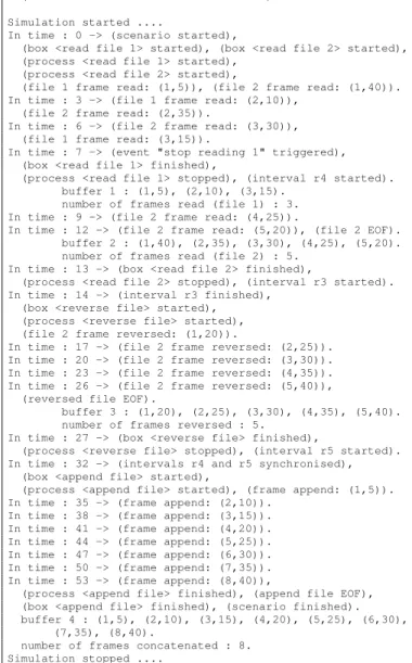
Now, we emphasize the main events generated in the report. At 7 milliseconds the box for reading the first file was stopped by the performer, then only 3 frames of the file were read. Observe that each frame was processed preserving the corresponding delay (i.e., 3 milliseconds). At 12 milliseconds the second files was completely read, but the box finished at 13 milliseconds. Note that the output of a process is buffered in order to be read later by another process. At 14 milliseconds, the second file started to reverse and finished at 26 milliseconds. At 32 milliseconds all preceding intervals of the box for appending files were satisfied and the box started to concatenated the first file and the reversed second file. Finally, the process finished at 53 milliseconds, then the box also was stopped at the same time. Notice that the output of the above process corresponds correctly to the transformations applied to files read at the beginning of the scenario.

time (ms) 0 1 2 3 4 5 6 7 8 9 10 11 12 13 14 15 16 17 18 19 20 21 22 23 24 25 26 27 f1 f2 f3 f4 f5 f1 f2 f3 f4 f5 28 29 30 31 32 min max f1 f2 f3 33 34 35 36 37 38 39 40 41 42 43 44 45 46 47 48 49 50 51 52 53 f4 f5 f6 f7 f8 54 55 56 57 58 f1 f2 f3 min max

Read File 1 (process) Read File 1 (box)

Read File 2 (process) Read File 2 (box)

r3

Reverse File (process) Reverse File (box)

r5

Append Files (process)

Append Files (box) r4

(10)

Hence, comparing the simulation report in Figure 22 with the execution time-line in Figure 22, we observe that our model executed correctly the scenario and preserved the temporal or-ganization of the score during execution. Moreover, it follows

the execution model of I-SCORE and also allows to handle

complex data such as audio streams.

V. CONCLUDINGREMARKS

In this paper we presented a model to execute interactive scores [1] with the ability to handle complex data, in particular, data audio streams. We used Coloured Petri Nets [4] to model audio frames as coloured tokens that are handled by processes. These processes have inputs and outputs, and they can pass values between them through intervals. The above allows the functional composition of processes. We took advantage of this functional composition and the hierarchy support of CPNs to

build a modular model. Thus, we extended the model of the I

-SCORE software with modules for processing audio files such as reading, appending and reversing files.

We illustrated the notion of asynchronous functional com-position of our model by simulating the scenario shown in Figure 21. Here, the outputs of the modules for reversing and appending files are buffered before the module for appending files starts. Also, we implemented a method for merging inter-vals which allows to translate any temporal property defined by the user into our model. We implemented our model in CPNTOOLS, and then we simulated a scenario that allows to observe that our approach models interactive scores and audio streams correctly.

Future Work. Interactive scores have a wide range of applications in all types of industries, for example, video games, live performance installations, and virtual museum visits [8]. The use of loops and conditionals are necessary for the proper design of scenarios for these kind of applications.

However, the model of I-SCORE does not support them. We

plan to take advantage of the capability of our model for handling complex data and the power of the CPN formalism to model these features. In a first approach, we could represent conditionals like the switch statement of the C programming language where: each case could be the guard of a set of transitions that have associated a sub-scenario; and a coloured token that carries the value that will be compared. Therefore, the transition whose guard is fulfilled with the value of the token will execute the corresponding sub-scenario. We could represent loops like a hierarchical box that executes its children until a specific condition is false. Note that, the implementation of loops requires conditionals.

Additionally, audio processing is very important in the applications listed above. Then, we plan to extend our model with new audio processing processes. For example, we could change the play speed of an audio by modifying the interval of time in which the module for reading files reads each frame. Also, we could amplify the audio volume by scaling the values of each read frame.

Finally, we plan to verify properties about scenarios like the maximum number of processes that can be executed at the same time in a specific machine, the maximum duration of the buffers, the maximum duration of the scenario, among others.

Example Scenario with Audio Processing ====================================== Parameters ...

Box <read file 1> duration:

(min: 6 time units), (max: 9 time units). Box <read file 2> duration: 13 time units. Box <append file> duration:

(min: 0 time units), (max: 25 time units). Box <reverse file> duration: 13 time units. Interval r4 duration: 3 time units. Interval r3 duration: 1 time units. Interval r5 duration: 5 time units.

Process <read file 1>: (max. n. frames: 4 frames), (frame duration: 3 time units),

(data: [(1,5), (2,10), (3,15), (4,20)]). Process <read file 2>: (max. n. frames: 5 frames),

(frame duration: 3 time units),

(data: [(1,40), (2,35), (3,30), (4,25), (5,20)]). Process <reverse file>: (frame duration: 3 time units). Process <append file>:

(frame duration file 1: 3 time units), (frame duration file 2: 3 time units). Simulation started ....

In time : 0 -> (scenario started),

(box <read file 1> started), (box <read file 2> started), (process <read file 1> started),

(process <read file 2> started),

(file 1 frame read: (1,5)), (file 2 frame read: (1,40)). In time : 3 -> (file 1 frame read: (2,10)),

(file 2 frame read: (2,35)).

In time : 6 -> (file 2 frame read: (3,30)), (file 1 frame read: (3,15)).

In time : 7 -> (event "stop reading 1" triggered), (box <read file 1> finished),

(process <read file 1> stopped), (interval r4 started). buffer 1 : (1,5), (2,10), (3,15).

number of frames read (file 1) : 3. In time : 9 -> (file 2 frame read: (4,25)).

In time : 12 -> (file 2 frame read: (5,20)), (file 2 EOF). buffer 2 : (1,40), (2,35), (3,30), (4,25), (5,20). number of frames read (file 2) : 5.

In time : 13 -> (box <read file 2> finished),

(process <read file 2> stopped), (interval r3 started). In time : 14 -> (interval r3 finished),

(box <reverse file> started), (process <reverse file> started), (file 2 frame reversed: (1,20)).

In time : 17 -> (file 2 frame reversed: (2,25)). In time : 20 -> (file 2 frame reversed: (3,30)). In time : 23 -> (file 2 frame reversed: (4,35)). In time : 26 -> (file 2 frame reversed: (5,40)),

(reversed file EOF).

buffer 3 : (1,20), (2,25), (3,30), (4,35), (5,40). number of frames reversed : 5.

In time : 27 -> (box <reverse file> finished),

(process <reverse file> stopped), (interval r5 started). In time : 32 -> (intervals r4 and r5 synchronised),

(box <append file> started),

(process <append file> started), (frame append: (1,5)). In time : 35 -> (frame append: (2,10)).

In time : 38 -> (frame append: (3,15)). In time : 41 -> (frame append: (4,20)). In time : 44 -> (frame append: (5,25)). In time : 47 -> (frame append: (6,30)). In time : 50 -> (frame append: (7,35)). In time : 53 -> (frame append: (8,40)),

(process <append file> finished), (append file EOF), (box <append file> finished), (scenario finished). buffer 4 : (1,5), (2,10), (3,15), (4,20), (5,25), (6,30),

(7,35), (8,40).

number of frames concatenated : 8. Simulation stopped ....

Fig. 22. Simulation report of an execution of the score shown in Figure 21.

ACKNOWLEDGMENTS

We thank the anonymous reviewers for their detailed com-ments that helped us to improve this paper. This work has been

(11)

supported by the OSSIA (ANR-12-CORD-0024) project and

SCRIME6.

REFERENCES

[1] A. Allombert, “Aspects temporels d’un syst`eme de partitions musicales interactives pour la composition et l’ex´ecution.”

[2] R. Marczak, M. Desainte-Catherine, and A. Allombert, “Real-time temporal control of musical processes,” in The Third International Conferences on Advances in Multimedia, ser. MMEDIA 2011, pp. 12–17. [3] P. S´enac, P. de Saqui-Sannes, and R. Willrich, Hierarchical Time Stream Petri Net: A Model for Hypermedia Systems, ser. Lecture Notes in Computer Science. Springer Berlin Heidelberg, vol. 935, pp. 451–470. [4] K. Jensen and L. M. Kristensen, Coloured Petri Nets. Modelling and Validation of Concurrent Systems. Dordrecht; New York: Springer, 2009. [5] J. F. Allen, “Maintaining knowledge about temporal intervals,” vol. 26,

p. 832–843.

[6] G. Gallasch and L. M. Kristensen, “Comms/CPN: a communication infrastructure for external communication with Design/CPN,” in Third Workshop and Tutorial on Practical Use of Coloured Petri Nets and the CPN Tools. DAIMI PB-554, pp. 75–91.

[7] M. Desainte-Catherine, A. Allombert, and G. Assayag, “Towards a hybrid temporal paradigm for musical composition and performance: The case of musical interpretation,” Computer Music Journal, vol. 37, no. 2, pp. 61–72, 2013.

[8] A. Allombert, M. Desainte-Catherine, and G. Assayag, “Iscore: a system for writing interaction,” ser. DIMEA ’08. Athens, Greece: ACM, Sep. 2008, p. 360–367.