HAL Id: hal-01455151
https://hal.archives-ouvertes.fr/hal-01455151
Submitted on 3 Feb 2017
HAL is a multi-disciplinary open access
archive for the deposit and dissemination of
sci-entific research documents, whether they are
pub-lished or not. The documents may come from
teaching and research institutions in France or
abroad, or from public or private research centers.
L’archive ouverte pluridisciplinaire HAL, est
destinée au dépôt et à la diffusion de documents
scientifiques de niveau recherche, publiés ou non,
émanant des établissements d’enseignement et de
recherche français ou étrangers, des laboratoires
publics ou privés.
Method for Spectra Estimation from High-Speed
Experimental Data
Anne-Marie Schreyer, Lionel Larchevêque, Pierre Dupont
To cite this version:
Anne-Marie Schreyer, Lionel Larchevêque, Pierre Dupont. Method for Spectra Estimation from
High-Speed Experimental Data. AIAA Journal, American Institute of Aeronautics and Astronautics, 2016,
54 (2), pp.557-568. �10.2514/1.J054370�. �hal-01455151�
Method for spectra estimation from high-speed
experimental data at discrete points in time
Anne-Marie Schreyer,
∗Centre National d’Etudes Spatiales CNES, DLA, 75612 Paris Cedex, France
Lionel Larchevˆ
eque,
†and Pierre Dupont
‡Aix-Marseille Universit´e, IUSTI UMR 7343, 13013 Marseille, France
The present paper presents a technique to estimate spectra from experimental data sam-pled at discrete points in time. Our interest is to investigate spatio-temporal dependencies in supersonic turbulent flows like boundary layers and shock wave / turbulent boundary layer interactions. The experimental data are measured by means of a Dual–PIV system that gives access to a certain amount of temporal information also in high-speed flows.
The cross-correlation information in space made available by the Dual–PIV system can be used to reconstruct the auto-correlation for delay times ranging between the discrete points measured with the Dual–PIV system. This can be achieved for convection-dominated regions of the flow by moving into the convected frame of reference, similarly to Taylor’s hypothesis.
The principle and suitability of the suggested technique is demonstrated in a combined numerical-experimental approach. The LES simulations give access to fully time-resolved data and can thus be used to verify the accuracy of the auto-correlation and spectra esti-mated from experimental data. Also, the choice of time delays for the measurements can be optimized based on the numerical results.
Nomenclature
u Streamwise velocity component
x Position vector
x Streamwise coordinate
y Wall-normal coordinate
y+ Altitude in wall unit
U∞ External streamwise velocity
δ99 Boundary layer thickness
ξ Space distance vector
τ Time delay
τi Discrete time delay
Θk Set of discrete time delays
R Correlation function
r Correlation coefficient
C− Upstream convection velocity
C+ Downstream convection velocity
R− Retarded–time estimate of the auto-correlation function
R+ Advanced–time estimate of the auto-correlation function
∗Post-doctoral research fellow, Centre National d’Etudes Spatiales CNES, DLA, 75612 Paris Cedex, France, and IUSTI
UMR 7343, 13013 Marseille, France.
†Maˆıtre de Conf´erence, Institut Universitaire des Syst`emes Thermiques Industriels IUSTI, Aix–Marseille Universit´e and
UMR CNRS 7343, Marseille 13013, France.
‡Charg´e de Recherche, Institut Universitaire des Syst`emes Thermiques Industriels IUSTI, Aix–Marseille Universit´e and UMR
Rint Interpolated value of the auto-correlation function
∆x Cell dimension in the streamwise direction
h·i Time averaging operator
I.
Introduction
Shock-wave / turbulent boundary layer interactions occur in a large number of aerospace engineering applications with supersonic flow, such as rocket engine nozzles, supersonic and hypersonic vehicles, and air-breathing engine intakes. They feature a highly unsteady flow field, whose spatio-temporal development and investigation of frequency domain is of great interest to gain a deeper understanding of the flow field. Furthermore, the flow field that we intend to investigate, a reflected plane-shock interaction at Mach 2, has a large range of characteristic frequencies between O(100 Hz) for the shock motion and breathing pulsations of the separation bubble, O(1 − 10 kHz) for the mixing layer developing over the bubble, O(10 − 50 kHz) for
the incoming boundary layer and O(100 kHz) for the turbulent micro scales.10 The detailed analysis of this
class of flowfields consequently requires measurements systems of high space resolution that are also able to deal with such a wide range of time scales.
Particle Image Velocimetry (PIV) provides the velocity field in one entire plane, but no systems exist that are time-resolved in supersonic flows. Framing rates of up to 25 kHz were obtained in the system developed
by Wernet.32 Considering for instance a supersonic boundary layer, the sampling frequencies available with
this system correspond to about 50% of the boundary layer’s characteristic frequency U∞/δ99, whereas it
should be as high as 10 U∞/δ99 in order to prevent any aliasing (see for instance Ganapathisubramani et
al.14). The severity of this criterion is illustrated by the fact that the M = 2, Reθ' 5000 boundary layer
under consideration in the present paper would require a 500 kHz time-resolved PIV in order to meet it.
Scarano and Moore25 proposed to take advantage of the high spatial resolution of PIV systems so as to
supersample data in time through a refined Taylor hypothesis. This workaround however requires a large field
of view in the streamwise direction, whose length can be roughly estimated to be equal to O(10 δ99) based
on the above–estimated sampling frequency and with the assumption of a typical convection velocity equal
to U∞. Moreover, the extrapolation from space to time over such a large distance is strongly challenging the
validity of the “frozen turbulence” assumption from which the Taylor hypothesis is built.
More recent PIV setups2 may have up to two–time higher sampling rate, reducing the required field of
view by a factor of five. Such an improvement is however achieved at the expense of the spatial resolution of the PIV camera and the equivalent Nyquist frequency associated with the Taylor hypothesis is consequently
significantly reduced. Assuming a minimal convection velocity of 0.5 U∞, time supersampling without aliasing
would require measurement cells of streamwise dimension lower than δ99/20 in order to be able to reach an
equivalent sampling frequencies of 10 U∞/δ99. Even when taking into account the fact that the length of the
required field of view is reduced to 2 δ99 because of the higher sampling rate, the cell count is found to be
as high as 40 measurement cells in the streamwise direction, which is barely compatible with the 640 pixels
streamwise resolution in reference.2
With our newly developed Dual–PIV system,26 some temporal information can be obtained by
choos-ing an appropriate temporal delay between the two recordchoos-ings of the system. Such a set-up does not
allow the reconstruction of time–resolved flowfields but it can nonetheless be used to extract time–related information through the pointwise computation of velocity power spectra. However, to obtain complete spectral information, a large number of measurements at different temporal delays has to be performed, which means great experimental effort and costs.Therefore, the suggested method uses the spatio-temporal information contained in the Dual–PIV measurements to reconstruct temporal auto-correlations from spatial cross-correlations determined at each of the temporal delays δτ of the systems for which measurements were realized. To do so, the convection velocity of boundary layer structures is taken into account, similar to
Taylor’s hypothesis. This way, temporal correlations can be reconstructed at time delays δτi that slightly
differ from the measurement time delays δτ for regions in the flow field that are convection-dominated. Of course the time delays δτ for which measurements are performed have to be chosen sensibly.
To test and assure that the method can produce meaningful results in supersonic boundary layer flows, it was applied on numerical simulation data of a Mach 2 turbulent boundary layer from Large–Eddy Sim-ulation (LES). Furthermore, this combined experimental-numerical approach offers the means to test the possibilities and limitations of the method as well as to determine sensible parameters for the measurements.
It was then applied on PIV measurements in a Mach 2 turbulent boundary layer and results will be show in this paper, along with investigations on the number of time delays required for satisfactory accuracy and a comparison of different interpolation methods.
The contents of this paper are the following: in Sec. II, the idea and principle of the suggested recon-struction method is presented. Section III describes the experimental and numerical setups, including the measurement principle of the Dual–PIV system with which we collect the data on which the reconstruc-tion method will be applied (Sec. III.A), the setup for the measurements in a supersonic boundary layer (Sec. III.B.1), and finally the numerical setup for the boundary-layer study (Sec. III.B.2). The results the validation study base on numerical data are then presented in Sec. IV.A showing that the suggested re-construction technique can be applied in a supersonic boundary layer, and results based on experimental boundary-layer data are shown in Sec. IV.B. Conclusions and an outlook on future work follow in Sec. V.
II.
Principle of the method
Assuming that Dual–PIV measurements are available for a small number n of time delays τi, i = 1, . . . , n,
the cross-correlation function of the velocity R(x, ξ, τ ) between a reference location x and in its vicinity, defined by
R(x, ξ, τ ) = hu(x, t) u(x − ξ, t − τ )i − hu(x, t)i × hu(x − ξ, t − τ )i (1)
can be computed for both positive and negative time delays ±τi. The cross-correlation coefficient r(x, ξ, τ ),
defined by :
r(x, ξ, τ ) = R(x, ξ, τ )
pR(x, 0, 0) × R(x − ξ, 0, 0), (2)
can also be deduced from these measurements. The power spectra of the velocity u at location x then can be estimated directly by computing the time Fourier transform of R(x, 0, τ ), resulting in the Blackman–Tukey
correlogram.3 This spectral estimator will however yield very poor spectral resolution because of the low
value of n compatible with actual Dual–PIV constraints.
The idea of the present paper is to take advantage of the cross-correlation information in space made available by the Dual–PIV in order to reconstruct the auto-correlation in time. It can be achieved for convection–dominated regions of the flow by moving into the convected frame of reference, similarly to the Taylor hypothesis.
The convection velocity at the location x has first to be estimated. It is achieved by seeking, for every τi,
the location x − ξi for which r(x, ξ, τ ) is maximal. Note that in the present algorithm, sub-cell interpolation
of the location of the maxima is obtained through bi-quadratic interpolation over 3 × 3-cell subdomains. The
convection velocity is then estimated by performing a linear regression on the (x − ξi, τi) dataset restricted to
values of τifor which r(x, ξi, τi) is above a given threshold. If no time delay τj yielding a value of r(x, ξi, τi)
greater than the threshold can be found among the sampled time delays, the convection velocity is estimated
using the lowest value of τi being available. The threshold has been set to 0.4 in the present work based
on preliminary tests using LES databases of boundary layer and shock-boundary layer interaction flows.
Eventually, the convection velocities C+ and C−, associated with regions of the flow respectively located
downstream and upstream of x, are obtained by considering negative and positive values of τi, respectively.
Assuming convection in the upstream and downstream directions with convective velocities respectively
equal to C−and C+, the auto-correlation function R(x, 0, τ ) can be estimated for a given τ lying within the
interval [τj, τj+1] either by the advanced–time R+(x, τ ) or by the retarded–time R−(x, τ ) extrapolations.
These two estimates read : R+(x, τ ) = R[x, −C+× (τ − τj) , τj] , R−(x, τ ) = R[x, −C−× (τ − τj+1) , τj+1] . (3)
Two further estimates can be obtained by taking advantage of the evenness of the auto-correlation function, i. e. R(x, 0, τ ) = R(x, 0, −τ ). Considering a negative time delay −τ , these two extra estimates are given by:
R−(x, −τ ) = R[x, −C−× (−τ − τ−j) , τ−j] , R+(x, −τ ) = R[x, −C+× (−τ − τ−j−1) , τ−j−1] . (4)
If the flow is close to be homogeneous in the streamwise direction, the upstream estimates R− associated
with the convection velocity C− and the downstream estimates R+ associated with the convection velocity
C+ can be simply averaged. Note that other weighting schemes taking into account the value of the
corre-lation coefficient r(x, 0, τ ) for positive and negative time delays could be considered in order to achieve an upwind interpolation of better performance in non-homogeneous regions.
The two resulting estimates, interpolated respectively from the time delays τ±j and τ±j±1, can then be
simply linearly weighted using the function :
w(τ ) = τ − τj τj+1− τj
for estimates of Eq. 3
−τ − τ−j
τ−j−1− τ−j
for estimates of Eq. 4
(5)
resulting in the interpolated value :
Rint(x, 0, τ ) = [1 − w(τ )]
R−(x, −τ ) + R+(x, τ )
2 + w(τ )
R+(x, −τ ) + R−(x, τ )
2 (6)
which is equal to the exact known values R(x, 0, τ ) for τ = τj and τ = τj+1.
The accuracy of the interpolation thus defined over [τ−j−1, τ−j] and [τj, τj+1] can be estimated a priori
by looking at the known values of r(x, −C±× τ?, ±τ?), where τ? stand for the lowest value among the set
of time delays τi which is greater than τj+1− τj. A high value of this correlation coefficient is an indication
that the flowfield remains correlated over the time interval considered for the interpolation. Based on this
piece of information, it is possible to derive a strategy to define efficiently the values of τi that have to be
sampled by Dual–PIV. One has first to perform Dual–PIV sampling for very few values of τi being of the
same order of magnitude as the estimated typical convective timescale of the flow. Then, one has to select
τopt among this set of time delays by looking at the largest value of τi that result in higher–enough values
of r(x, −C±× τi, τi). Further time delays can then be added with values increased by τoptup to the desired
largest time delay. This is an improvement in flexibility over the time-resolved method described in25 for
which an inadequate sampling rate would make the full time series useless for spectral analysis and would require to perform, if possible, brand new measurements with a higher sampling rate.
Using the interpolation above–described method, auto-correlations R can be reconstructed using Rintfor
any arbitrary value of τ ∈ [0, maxiτi]. The auto-correlation thus reconstructed can be Fourier-transformed
in order to obtain a spectral estimate potentially having a higher resolution/bandwidth than the Blackman– Tukey correlogram computed from the (few) known exact values of R. Provided that the flow is dominated
by convection, the spectral estimator should be accurate up to the equivalent Nyquist frequency fconv
Nyquist
associated with the convection, which reads: fNyquistconv =
min (kC−k , kC+k)
2 ∆x , (7)
where ∆x stands for the dimension of the cell along the direction of convection.
It may be noted that for the spectrum estimate thus defined, supplementing the initial set of Dual–PIV measurements with measurements associated with larger time delays yields an extension of the estimate towards low frequencies but also an increase of its frequency resolution. However, contrary to the standard Blackman-Tukey correlogram computed from time series, the estimate does not face a trade-off between the frequency resolution and the statistical uncertainty: uncertainties are here solely induced by the statistical (lack of) convergence of the Dual–PIV measurements of the cross–correlation, which is inherently independent of the value of τ under consideration.
III.
Experimental and numerical setup
A. Measurement principle of the Dual–PIV system
In principle, Dual–PIV systems consist of two independent PIV systems observing the same field of view. Unlike classical time-resolved PIV systems featuring at best temporal resolutions of around O(25 kHz) with
of certain temporal information also in a high-speed flow, where frequencies greater than O(100 kHz) are required to resolve the turbulent microscales, and give insight into the temporal development of the flow while maintaining the same high spatial resolution as in classical PIV systems.
A number of Dual–PIV and dual-plane stereoscopic PIV systems have been developed in other research
groups,4, 5, 11, 12, 16–19, 23, 30–32 mainly differing in the image-separation approach, but also in laser power
and spatial resolution. The most-commonly used approach to separate the images is polarization based, a technique that also allows arbitrarily small time delays and is thus applicable for measurements in high-speed flows. The two laser beams are cross-polarized and the cameras are equipped with two different polarizers that either allow the passage of vertically or horizontally polarized light.
To achieve good data accuracy with polarization-based systems, spherical seeding particles are required
and therefore droplets should be used.23 However, in quite a few high-speed flow applications, solid
metal-oxide particles have shown favorable behavior and in exothermic reacting flows this type of particle is indispensable.
While oil droplets from incense smoke are the seeding material chosen in our application, we were still interested in the development of a more versatile PIV system that is independent of the chosen type of seeding particles. Based on these requirements, a new Dual–PIV system has been designed in collaboration with DantecDynamics.
The key technology of this system is thus frequency-based image separation: two lasers of different wave lengths illuminate the field of view. Image separation is achieved with color filters placed in front of the
cameras. This approach was chosen before by Mullin & Dahm,23 who developed a frequency-based image
separation system for their Dual-Plane Stereo PIV setup. They used a dual-head Nd:YAG laser at a wave length of 532 nm and two pulsed dye lasers at a wave length of 635 nm, which were again pulsed by two Nd:YAG laser tubes. Color filters on the lenses of the PIV cameras were applied to separate the images from each other. With this laser system, pulse energies of 40 mJ were obtained.
However, to obtain sufficient illumination with the small seeding particles necessary in high-speed flow, we required larger pulse energies. Also, to obtain high quality PIV data, we required two lasers with more similar characteristics and thus the same signal to noise ratio for both systems. Therefore, a dual head Nd:YAG laser operating at a wave length of 532 nm and a pulse energy of 200 mJ/pulse was used along with a specifically altered Nd:YLF laser, operating at an equally large pulse energy, but at the only slightly different wave length of 527 nm. To separate the images, we installed optical color filters, one low-pass and one narrow band-pass filter, in front of the camera lenses. The intensity ratios between the inter-system cross-pollution and the measurement signal were for f-stop ranging from 4 to 22. The color filter’s blockage was found to be above 96% to 99%. The image separation can thus be considered as more than sufficiently effective.
Two high-resolution 4008 × 2672 pixels dual-frame Hisense 630 (PCO 4000) cameras with high sensitivity CCD, having a minimum inter-frame delay of 200 ns and equipped with Zeiss 100 mm f2 objectives, are used. The large sensor gives a high sensitivity and thus allows the use of small seeding particles that faithfully follow the flow. At the same time, we can obtain a large field of view, that is compatible with the extended flow field of a separated shock wave /turbulent boundary layer interaction while maintaining a high spatial resolution of 35 pixels/mm.
A high-accuracy dual camera mount with a cubic prism assures that the two cameras, which are installed perpendicular to each other, view the same field of view. Displacements in the registration of the fields of
view of only O(2-3pixels) between the two cameras can be obtained over the full range26 with no significant
rotation between the two frames.
A Fast Digital Converter is used for the synchronization of the system. The time delay between the two camera and laser systems can be arbitrarily chosen between 0 ≤ δτ ≤ ∞, with an error smaller than 10 ns,
which is acceptable for high speed flows. For further details on the system refer to Schreyer et al.26, 27
B. Supersonic boundary layer
1. Experiments
The measurements were performed in the supersonic wind tunnel at the IUSTI laboratory at a Mach number of M = 2. This hypo-turbulent wind tunnel is a continuous facility with a closed-loop circuit. The facility has been used for detailed investigations in supersonic boundary layers and extensive shock wave/boundary
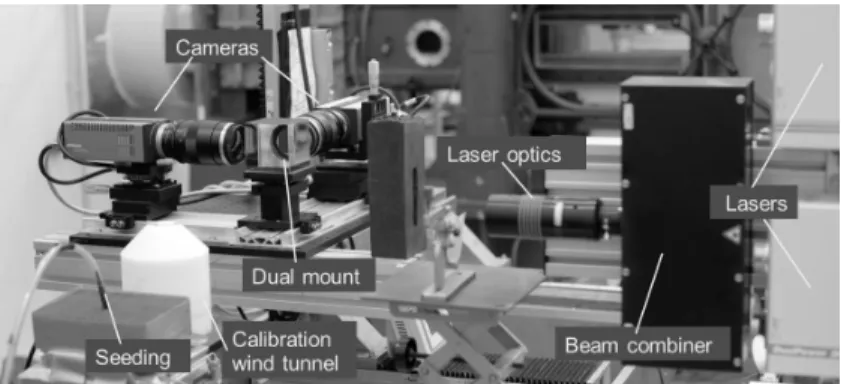
Figure 1. Setup of the Dual–PIV system at IUSTI for the calibration jet used during system development
(see Schreyer et al.26).
Figure 2. Schematic of the supersonic setup of the Dual–PIV system at IUSTI.
are using a Mach 2 nozzle with a rectangular test section having a width of 170 mm and a height of 105 mm to investigate the boundary layer developing on the test section floor.
The existing Dual–PIV setup shown in Fig. 1, consisting of the two cameras and the dual-mount prism
installed on a Thorlabs optical breadboard, has been described in detail and validated in Schreyer et al.26 It
is placed in front of the optical window in the side wall of the wind-tunnel test section. The laser light–sheet enters the test section via a second optical window further downstream and is redirected to the appropriate location in the flow field by means of a prism mounted downstream of the test section in the diffuser of the wind tunnel so as to illuminate a streamwise–wall normal–aligned field of view: see Fig. 2 for a schematic drawing.
Seeding near–wall regions of supersonic turbulent boundary layer is challenging since any wake induced by the seeding devices can affect the region far downstream of the seeding location. In order to minimize flow perturbations, the boundary layer is seeded through openings in the wind tunnel floor upstream of the nozzle: the flow outside of the boundary layer is thus not seeded. Such a system nonetheless leads to a quite homogeneous seeding of the turbulent boundary layer (see Fig. 3) while minimizing the downstream influence of the seeding device on the near–wall properties of the boundary layer, as verified from hot–wire measurements.
The experimental conditions for the present investigations are summarized in Table 1 and the boundary layer characteristics are summarized in Table 2. The data are derived from 1000 image pairs with a spatial
resolution of 35.1pixelmm, with a minimum interrogation window size of 32 × 16 pixels at 50% overlap. The
delay time between the two frames of the cameras was set to 1 µs. Considering a resolution of one tenth of
a pixel for the PIV measurements, it leads to an error of about 3 m.s−1 on the velocity, corresponding to
0.6% of the external velocity.
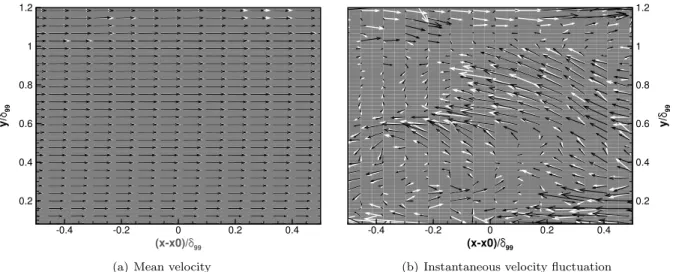
The efficiency of the dual-PIV system can be assessed by looking at the vector plots of Fig. 3. The mean velocity field computed either from camera C1 or camera C2 data are found nearly identical in the seeded
Table 1. Experimental conditions for the Mach 2 boundary layer experiment. The given quantities are: Mach
number M , free-stream velocity Ue at the boundary layer edge, momentum-thickness based Reynolds number
Reθ, stagnation pressure p0, and stagnation temperature T0.
M Ue Reθ p0 T0
1.98 506 m.s−1 4850 0.4 atm 290 K
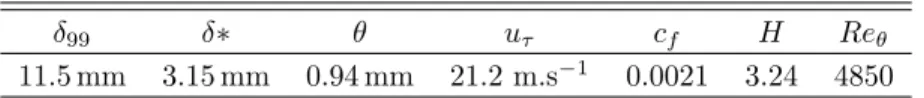
Table 2. Characteristics of the incoming turbulent boundary layer at Mach 2. The given quantities are:
Boundary layer thickness δ99, displacement thickness δ∗, momentum thickness θ, friction velocity uτ, friction
coefficient cf, shape factor H, and momentum-thickness based Reynolds number Reθ.
δ99 δ∗ θ uτ cf H Reθ
11.5 mm 3.15 mm 0.94 mm 21.2 m.s−1 0.0021 3.24 4850
region of the flow, as seen in Fig. 3(a). Moreover, Fig. 3(b) shows that when a zero time delay is set between the two cameras, the instantaneous fluctuating vector fields obtained from each of the two cameras display a high level correlation, as expected.
Boundary layer profiles are presented in Figs. 4(a) to 4(b) to demonstrate the quality of the newly-developed Dual–PIV system and to characterize the flow field for which the spectra-reconstruction technique will be demonstrated. The profiles are not spatially averaged and thus smooth curves and full statistical convergence are not to expect from only 1000 images. However, it can still be demonstrated that the system
provides high quality PIV data and allows accurate measurements of the Reynolds shear stresses u0v0, which
is extremely difficult to measure and resolve correctly.29
The mean velocity profile transformed according to van Driest is shown in Fig. 4(a), and the profile shows the expected good agreement with the log-law
U+ =1
klog(Y
+) + C
with k = 0.41 and C = 5.25 between 80 ≤ Y+≤ 200 (see Smits & Dussauge29).
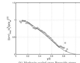
The turbulent Reynolds stress across the boundary layer in Morkovin scaling is compared to incompress-ible boundary layer measurements in Fig. 4(b) and shows the expected trends. As mentioned above, the flow outside the boundary layer is not seeded and thus the number of valid vectors gets smaller towards the
edge of the boundary layer. The Reynolds shear stresses u0v0 follow the subsonic value across the boundary
layer. Despite the low number of images from which these preliminary profile plots were deduced, the results clearly show fairly accurate measurements of a fully developed supersonic turbulent boundary layer.
2. Large-Eddy Simulation
A Large–Eddy Simulation (LES) matching the flow parameters of the experiments in supersonic flow has
been carried out in order to collect time–resolved data for a M=2.0 boundary layer with Reθ= 5000. The
computational domain has been chosen long enough to allow the simulation of a by-passed transition process in order to avoid spectral distortions that could be induced by unsteady turbulent inflow conditions. The transition is triggered by adding low-amplitude velocity perturbations to a laminar profile at the inflow, with
RMS values lower than 5 × 10⁻³U∞.
Dimensions of the domain are equal to 70 δ99, 8 δ99 and 1.2 δ99in the streamwise, wall–normal and
span-wise directions, respectively, with δ99 = 10.9 mm denoting the boundary layer thickness at the streamwise
location of interest, where Reθ = 5000. The transition process starts 9 δ99 downstream of the inflow and is
fully achieved 6 δ99further downstream. The location at which Reθreaches 5000 is found 55 δ99donwstream
of the inflow.
The grid resolution matches the requirement for wall-resolved LES, with respectively ∆x+ ' 30 and
∆z+' 12 in the streamwise and spanwise directions. The height of the cell adjacent to the wall is y+
1 ' 0.9
and 115 cells are located within the boundary layer thickness δ99. The total cell count is equal to 39 millions.
The computation is performed by means of ONERA’s FLU3M solver well-suited for supersonic turbulent
(x-x0)/ 99 y /9 9 -0.4 -0.2 0 0.2 0.4 0.2 0.4 0.6 0.8 1 1.2
(a) Mean velocity
(x-x0)/ 99 y /9 9 -0.4 -0.2 0 0.2 0.4 0.2 0.4 0.6 0.8 1 1.2
(b) Instantaneous velocity fluctuation
Figure 3. Velocity vector fields computed from measurements relying on each of the two independent PIV
cameras C1 (white) and C2 (black) in the Dual-PIV system with δτ = 0. One vector out of two is plotted in each direction, non-validated vectors being ruled out.
centered–Roe scheme. The hybridisation is achieved through the use of the Ducros sensor8 and the subgrid–
scale model is the selective mixed–scale model.21
Data have been sampled volumetrically over 9.8 ms, a value which corresponds to about 500 characteristic
timescales δ99/U∞. The sampling rate of 404 kHz has been chosen high enough to avoid any significant
spectral aliasing.
IV.
Results
A. Validation and parametrization based on LES data
The LES dataset enables to compute reliable power spectra of the velocity for a frequency range spanning more than two orders of magnitude. Moreover, since the data have been sampled with a high sampling rate, it gives a large flexibility in choosing time–delay subsets from which the correlations are computed, in a similar way a Dual–PIV system does. However, contrary to Dual–PIV measurements, choices of time delays can be made a posteriori without requiring further time–consuming data sampling. Consequently the LES data are used to study parametrically the influence of the sampling–set definition on the interpolation scheme defined by Eq. 6. Using this scheme, auto-correlation functions are reconstructed using exact values sampled at a given subset of time delays up to the complete set of time delays associated with the sampling rate of the LES. This reconstruction will be compared with the true auto-correlation function computed from the LES data as well as with linear and cubic-spline interpolations from the time–delay subset under consideration.
The reconstructed auto-correlations and the subsequent power spectra are computed for three different
altitudes. The first virtual sensor is located at altitude y+ = 15, where the turbulent kinetic energy is
maximal, the second one lies at the upper bound of the logarithmic region, with y+= 220 and y = 0.25 δ99,
and the third one is located above the boundary layer, in the intermittency region, with y = 1.1 δ99. The
corresponding convective velocities are equal to (kC+k , kC−k) = (0.449 U∞, 0.309 U∞), kC+k = kC−k =
0.775 U∞ and kC+k = kC−k = 0.975 U∞, respectively. Based on these values, the estimated Nyquist
frequency of the reconstructed spectra, computed using Eq. 7, are respectively equal to 244 kHz, 611 kHz and 769 kHz. The two latter values are well above the Nyquist frequency computed from the sampling rate
of the data, equal to 204 kHz, However, for y+ = 15, the two Nyquist frequencies are of the same order
of magnitude. This, coupled to the fact that, for this altitude, the convective velocity varies significantly when moving from the upstream zone to the downstream one because of the sweep/ejection process, make the location closest to the wall the most challenging for the interpolation scheme using the cross-correlation data.
102 103 12 14 16 18 20 22 24 26 28 Y+ U +
(a) Van Driest–transformed mean velocity
0 0.2 0.4 0.6 0.8 1 0 0.5 1 1.5 y/δ ((u , v , )rms /u 2 )(τ ρ /ρw ) 0.5
(b) Morkovin–scaled cross Reynolds stress
Figure 4. Profile of the mean velocity U transformed according to van Driest (left) and of the turbulent
Reynolds stresses u0v0in Morkovin scaling (right). Present PIV measurements are denoted by circle. The solid
lines respectively correspond to the log-law (left) and the subsonic data from Klebanoff20 (right).
Table 3. Definition of the five sets Θk of the time delays τi used to compute the interpolation of the
auto-correlation function. The total number of time delays encompassed by each set is given in the first column, next to the set name.
τi(µs.) 4.9 9.8 14.7 19.6 29.4 39.2 58.8 78.4 98 117.6 137.2 156.8 176.4 196.0 235.2, 274.4 313.6, 352.8 392.0 Θ1(14) × × × × × × × × × × × × × × Θ2(16) × × × × × × × × × × × × Θ3(10) × × × × × × × × × × Θ4(10) × × × × × × Θ5(11) × × × × × × ×
Five sets Θk of discrete time delays have been tested. The time delays τi they include are listed in
Tab. 3. Sets Θ3 and Θ4 correspond to uniform samplings of the auto/cross–correlation functions with
timesteps respectively equal to 20 µs and 40 µs. Note that these timesteps are very large with respect to
the physics of the flow since they are respectively equal to two and four characteristic time scales U∞/δ99
of the boundary layer. The doubled timestep of set Θ4 with respect to the one of set Θ3 enables to double
the largest value of τ using the same number of time delays, giving access to both twice a finer frequency resolution and twice a lower frequency for the spectral estimate. This frequency should be small enough to
resolve the plateau of the velocity spectra. Sets Θ1 and Θ2 add extra time delays of low τ values to sets
Θ3 and Θ4 in order to better resolve the auto-correlation function in the region where interpolation errors
have a strong impact on the computed value of the integral time-scale. Lastly, the time delays of set Θ4are
supplemented by one time delay in set Θ5 so as to remove a deficiency that will be described hereafter.
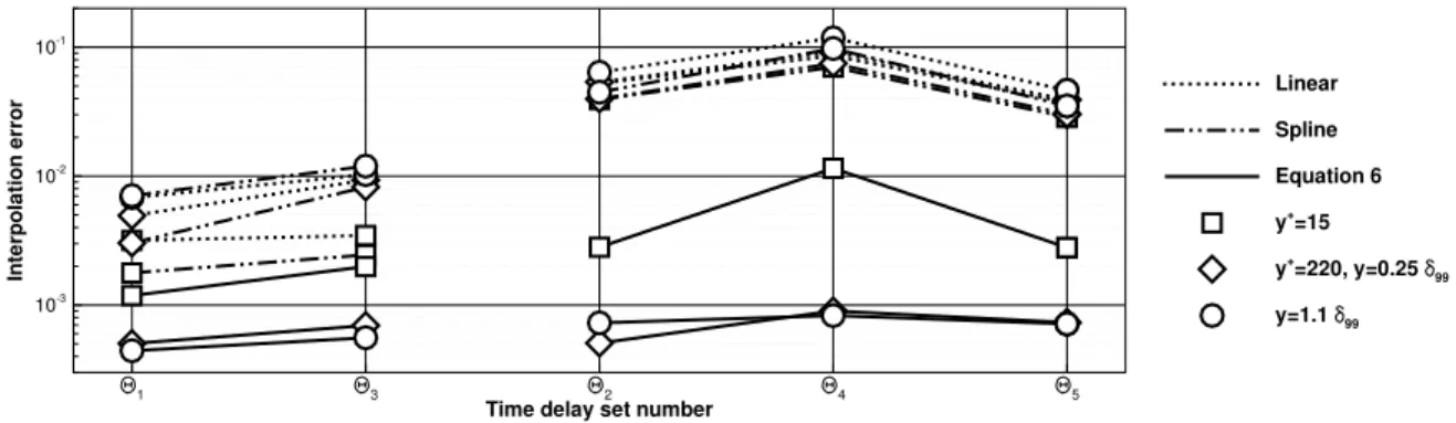
The RMS of the interpolation error, defined as the difference between the values of the auto-correlation coefficient computed from the LES data at the full sampling rate and the values of the auto-correlation
coefficient reconstructed by interpolating from subsets Θk, is plotted in Fig. 5. Note that measuring the
interpolation error using the L∞norm rather than the RMS value results in plots with similar trends as the
ones seen in Fig. 5. The sets Θ1and Θ2, refined in the low τ region, yield the better results. Unsurprisingly,
cubic spline interpolations result in lower error levels than linear interpolations. The cubic spline scheme is nonetheless outperformed by the cross–correlation–based scheme whatever the location under consideration.
Time delay set number In te rp o la ti o n e rr o r 1 3 2 4 5 10-3 10-2 10-1 Linear Spline Equation 6 y+ =15 y+ =220, y=0.25 99 y=1.1 99
Figure 5. RMS of the interpolation error for the sets of time delays defined in Tab. 3.
(s.) r( x ,0 , )
0.0E+00 2.0E-05 4.0E-05
0 0.2 0.4 0.6 0.8 1 Exact Linear ( 4) Spline ( 4) Equation 6 ( 4) Equation 6 ( 5) (a) Autocorrelation f (Hz) P S Du ( A rb it ra ry s c a le ) 103 104 105 10-8 10-7 10-6 10-5 10-4 Exact Linear ( 4) Spline ( 4) Equation 6 ( 4) Equation 6 ( 5) (b) Power Spectrum
Figure 6. Example at location y+ = 15 of some errors induced by the interpolation schemes and of their
consequences on the spectrum estimation.
of magnitude for both the linear and cubic spline interpolations. The increase is much milder for the
interpolation using the cross–correlation, with the exception of the location y+ = 15 for the set Θ4. For
these location and set, the cross correlation–based interpolation yields an error 6 times lower that the error of the spline interpolation whereas for the other locations the error levels of the cross correlation–based interpolations are at least one order of magnitude lower than their linear/cubic spline counterparts.
The main sources of interpolation errors can be identify by looking at Fig. 6. They are mainly due to an alteration of the auto-correlation shape in the low time–delay region. For the linear and cubic spline interpolations, this is a consequence of the severe undersampling of the auto-correlation function associated
with sets Θ2 and Θ4. As seen from the dotted and dashed–dotted curves on the left plot of Fig. 6, it
induces typical spurious increases of the integral timescale by factors of two (set Θ2) to four (set Θ4). Such
an overestimation of the integral time scale translates in the spectral domain into an overestimation of the power density level for the low–frequency region, as seen on the right plot of Fig. 6. This, in turn, yields an underestimation of the power density in the high–frequency region since the integral of the power spectrum over the whole frequency range, being equal to R(x, 0, 0), is kept unaltered by all the interpolation schemes. The linear interpolation scheme adds to this underestimation Gibbs-like oscillations typical of low–smoothness interpolations.
The cross-correlation–based interpolation scheme is not affected by the undersampling. The largest error
found in Fig. 5, for set Θ4 at location y+= 15, is nonetheless associated with an alteration of the main lobe
of the auto-correlation function, although in a much weaker way than for the linear and cubic spline schemes. The integral time scale is slightly underestimated, resulting in slightly underestimated/overestimated values of the power density for low/high frequencies, as seen from the solid curves in Fig. 6. These spurious effects
are the consequence of slightly inaccurate values of the convection velocities C+ and C−. It is due to the
f (Hz) P S Du ( A rb it ra ry s c a le ) 103 104 105 10-7 10-6 10-5 10-4 Exact Linear Spline Equation 6
(a) Locally refined set Θ1
f (Hz) P S Du ( A rb it ra ry s c a le ) 103 104 105 10-7 10-6 10-5 10-4 Exact Linear Spline Equation 6
(b) Locally refined set Θ2
f (Hz) P S Du ( A rb it ra ry s c a le ) 103 104 105 10-7 10-6 10-5 10-4 Exact Linear Spline Equation 6
(c) Uniformly sampled set Θ3
f (Hz) P S Du ( A rb it ra ry s c a le ) 103 104 105 10-7 10-6 10-5 10-4 Exact Linear Spline Equation 6
(d) Uniformly sampled set Θ4
Figure 7. Power spectra computed from the reconstruction of the auto-correlation function at altitude y+= 15.
the maximal value of r(x, ξ, τ ) is rather low, being equal to 0.2.
The largest value of τ that yields, for location y+ = 15, a maximal value of r(x, ξ, τ ) being above the
0.4 threshold is τ = 19.6 µs. Adding this value to set Θ4 results in set Θ5. The cross–correlation–based
interpolation using this set no longer suffers the aforementioned deficiency, as seen from the dashed curves
in Fig. 6 and from the reduced error level in Fig. 5 when moving from set Θ4 to set Θ5. The use of set Θ5
with linear and spline interpolations also yields an improvement compared to the results obtained with set
Θ4, as seen in Fig. 5. However the interpolated autocorrelations still suffer from an overestimations of the
integral time scale, resulting in noticeable distortion of the power spectra.
One has eventually to note that for the other tested locations, maximal values of r(x, ξ, 39.2 µs.) are above
the 0.4 threshold and that moving from set Θ4to set Θ5does not reduce significantly the interpolation error
for the cross-correlation–based interpolation scheme. It indicates that the value of r(x, ξ, τ ) obtained for the largest τ effectively used in the computation of the convection velocity is an efficient metric when a priori estimating the quality of the interpolation. It also indicates that a threshold of 0.4 is a reasonable limit to define the subset of necessary delay times for the experiments.
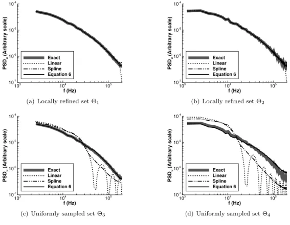
The accuracy of the spectrum estimators obtained from the interpolation of the auto-correlation function
can be assessed by looking at Figs. 7–9. As mentioned previously, the y+ = 15 location is the most severe
test for the reconstruction scheme for the high frequencies since it corresponds to the lowest value of 231 kHz for the equivalent Nyquist frequency obtained from Eq. 7. The solid curves in Fig. 7 nonetheless demonstrate that the reconstruction is accurate up to the highest available frequency of 204 kHz for both the refined sets
Θ1and Θ2and the uniformly sampled set Θ3. This is an indication of the ability of the interpolation scheme
to reconstruct the spectrum up to the equivalent Nyquist frequency.
Note that the high-frequency overestimation seen for set Θ4 is not induced by this equivalent Nyquist
frequency but rather by the above–mentioned inaccurate estimation of the convection velocity. This assertion
can be verified by looking at the dashed line of Fig. 6, obtained from set Θ5, which exhibits the same level of
accuracy than the reconstructions from sets Θ1–Θ3. It may therefore be concluded that beside that effect,
the choice of the time–delay set has no significant influence on the accuracy of the spectra computed using the cross-correlation–based interpolation.
f (Hz) P S Du ( A rb it ra ry s c a le ) 103 104 105 10-7 10-6 10-5 10-4 Exact Linear Spline Equation 6
(a) Locally refined set Θ1
f (Hz) P S Du ( A rb it ra ry s c a le ) 103 104 105 10-7 10-6 10-5 10-4 Exact Linear Spline Equation 6
(b) Locally refined set Θ2
f (Hz) P S Du ( A rb it ra ry s c a le ) 103 104 105 10-7 10-6 10-5 10-4 Exact Linear Spline Equation 6
(c) Uniformly sampled set Θ3
f (Hz) P S Du ( A rb it ra ry s c a le ) 103 104 105 10-7 10-6 10-5 10-4 Exact Linear Spline Equation 6
(d) Uniformly sampled set Θ4
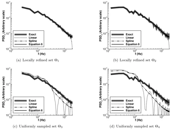
Figure 8. Power spectra computed from the reconstruction of the auto-correlation function at altitude (y+=
220, y = 0.25 δ99).
The linear reconstructions from the refined sets Θ1 and Θ2 suffer from a slight high frequency damping
whereas the spectra obtained from the cubic spline scheme applied to the same sets exhibit a slight overesti-mation in the same region. Both methods results in severe spectrum distortions when the uniformly sampled
sets Θ2 and Θ4 are considered, as analyzed previously.
When moving to higher altitudes that are free from the inaccuracy on the convection velocity encountered
at y+= 15 for the set Θ
4, Figs. 8 and 9 demonstrate that, whatever the time–delay set under consideration,
the spectra obtained for the cross–correlation–based interpolation are uniformly in excellent agreement with the exact spectra. On the contrary, the linear and cubic spline interpolations may lead to some errors in the
high–frequency regions even for the refined sets Θ1 and Θ2. Note that, based on spectrum reconstructions
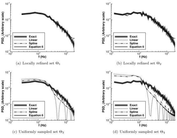
for several other altitudes than the ones presented in the this paper, the errors appears to be randomly distributed between over– and understimations. As a consequence, the good agreement found between the
cubic spline–based reconstruction and the exact spectrum for (y+ = 220, y = 0.25 δ99) (see Fig. 8) may
be purely accidental. An additional, slight, low-frequency alterations is found with set Θ2 for the sensor
located in the intermittency region, as seen on the left plot of Fig. 9. It denotes a moderate inability of these schemes to reconstruct the auto-correlation for large time delays. When the uniformly sampled sets
Θ3and Θ4 are considered, the strong amplifications/dampings of the low/high frequencies seen at y+= 15
are recovered for (y+= 220, y = 0.25 δ
99) and y = 1.1 δ99.
Based on the results of Fig. 7–9, the cross–correlation interpolation scheme allows, for all the loca-tions considered, the accurate reconstruction of the streamwise velocity power spectrum with a bandwidth h 1 20 U∞ δ99, 3 U∞ δ99 i
of almost a two orders of magnitude width using only six time delays (the first six ones of
set Θ5 listed in Tab. 3). An optimization of the time-delay set conducted for the cubic-spline interpolation
showed that it requires at least nine finely–tuned time delays to achieve a RMS interpolation error that, at best, matches the worse RMS error obtained with the cross–correlation interpolation using the above-mentioned 6–time delays set. Moreover, despite the inclusion of a very short time delay of 2.45 µs. in the optimized set, the resulting spectra still exhibit errors in the high–frequency range, although of lower
in-f (Hz) P S Du ( A rb it ra ry s c a le ) 103 104 105 10-7 10-6 10-5 10-4 Exact Linear Spline Equation 6
(a) Locally refined set Θ1
f (Hz) P S Du ( A rb it ra ry s c a le ) 103 104 105 10-7 10-6 10-5 10-4 Exact Linear Spline Equation 6
(b) Locally refined set Θ2
f (Hz) P S Du ( A rb it ra ry s c a le ) 103 104 105 10-7 10-6 10-5 10-4 Exact Linear Spline Equation 6
(c) Uniformly sampled set Θ3
f (Hz) P S Du ( A rb it ra ry s c a le ) 103 104 105 10-7 10-6 10-5 10-4 Exact Linear Spline Equation 6
(d) Uniformly sampled set Θ4
Figure 9. Power spectra computed from the reconstruction of the auto-correlation function at the altitude
y = 1.1 δ99.
terpolations based on a purely mathematical approach are not able to reconstruct the missing scales in an universal way when no additional information are available.
On the contrary, the spectra computed from the cross-correlation interpolation are accurate over the whole frequency range. Based on this fact, it is possible to estimate the cell count required in the streamwise
direction in order to achieve a two orders of magnitude–wide bandwith ranging from to 201 U∞
δ99 to 5 U∞
δ99. The
upper frequency bound would impose a cell dimension ∆x = δ99/40, based on formula 7 by assuming a
minimum convection velocity of U∞/4. The lower frequency bounds would require a maximum time delay
of 10δ99
U∞, yielding a maximum sampling timestep of ∆τmax = 2
δ99
U∞ if the same optimal uniform sampling
with five time delays as for the present study is retained. Assuming a maximum convection velocity equal
to U∞, the field of view of the PIV camera would have to encompass a domain of x ± 2 δ99. The cells count
would therefore be equal to 4 δ99×δ4099 = 160, a value which is within the reach of modern low– to medium–
sampling rate PIV systems. Note that under the same assumptions, the method described in Scarano et al25
used with a sampling frequency of 0.1 U∞/δ99would require from a high–sampling rate camera the far more
challenging cell count of about 10 δ99×δ4099 = 400.
B. Application to Dual–PIV measurements
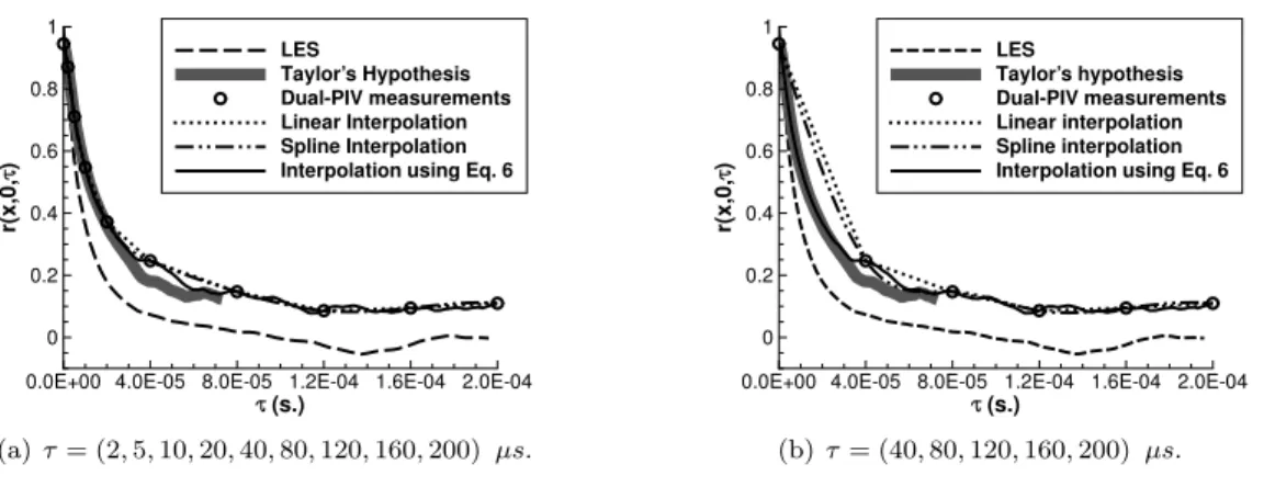
Figures 10 (a) and (b) show the auto-correlation coefficient (black symbols) determined from measurements with the two PIV cameras C1 and C2 in the supersonic boundary layer for two sets of temporal delays. The overall system noise – determined from the deviation of the auto-correlation coefficient at δτ = 0 from unity – is below 5% (2.5% when considering standard deviations) in the Mach 2 turbulent boundary layer, and
thus slightly above the value found for a much less noisier subsonic jet flow.26, 27 Such a high correlation
level at δτ = 0 quantitatively confirm the qualitative results obtained from Fig. 3(b).
The results for temporal delays between 0 ≤ δτ ≤ 200 µs are shown for location yδ = 0.25 in the boundary
layer, where a velocity fluctuation level of uU0 = 9.6% prevails. The choice of appropriate time delays was
(s.) r( x ,0 , )
0.0E+00 4.0E-05 8.0E-05 1.2E-04 1.6E-04 2.0E-04 0 0.2 0.4 0.6 0.8 1 LES Taylor’s Hypothesis Dual-PIV measurements Linear Interpolation Spline Interpolation Interpolation using Eq. 6
(a) τ = (2, 5, 10, 20, 40, 80, 120, 160, 200) µs. (s.) r( x ,0 , )
0.0E+00 4.0E-05 8.0E-05 1.2E-04 1.6E-04 2.0E-04 0 0.2 0.4 0.6 0.8 1 LES Taylor’s hypothesis Dual-PIV measurements Linear interpolation Spline interpolation Interpolation using Eq. 6
(b) τ = (40, 80, 120, 160, 200) µs.
Figure 10. Reconstruction of the auto-correlation coefficient based on PIV measurements with different meth-ods for two different selections of temporal delays.
decay of the auto-correlation coefficient in space, translated into the time domain using Taylor’s hypothesis, could also have been used to roughly estimated the acceptable maximum timestep of 40 µs, as seen from the thick gray line in Fig. 10. Note that the statistical uncertainty level of the data has been reduced by taking advantage of the streamwise quasi-homogeneity of the flow: the auto-correlation coefficients have been computed for seven locations distributed over a streamwise interval with a width of 0.24δ and the resulting seven estimates were then averaged. The auto-correlation function has been interpolated using the same methods as for the LES data (see Figs. 7-9).
Distortions of the linear and spline-based reconstructions are similar to the ones seen for the LES data in Fig. 6 while the trend of the auto-correlation function interpolated from the cross-correlation is as expected for a turbulent flat-plate boundary layer. However, the curve does not approach zero as fast as expected, leading to an overestimation of the integral time scale: a value of T ≈ 12 µs, corresponding to a characteristic frequency of f = 80 kHz, is determined from the experiment, while the LES data predict T = 6 µs.
The difference in decay could come from a low-frequency forcing specific to the wind tunnel, LES modeling errors or PIV measurement biases. Definitive answers for the two first items would require further extensive experiments and/or computations. Such refined analysis appears to be far beyond the scope of the present article, since it is unlikely that the presence of either a moderate low-frequency forcing in the experiment or modeling errors in LES will alter the rather robust Taylor hypothesis to the point of invalidating the reconstruction scheme built from it. Moreover, the large integral timescale found in the experiment can be inferred from the discrete measurements of the auto-correlation function (circles in Fig. 10), demonstrating that it is not induced by the reconstruction scheme.
Features inherent to the Dual–PIV technique or PIV in general could result in a bias of the auto–
correlation function towards large integral time scales. Different possible causes for a slow decay have
been identified and have been tested on the LES database and by means of experimental investigations. A first thinkable cause specific to the Dual–PIV technique is a crosstalk–disturbance effect between the two independent PIV systems, although the level of cross-pollution is very low for this Dual–PIV system
(see Schreyer et al.26). However the auto-correlation coefficient r(x, 0, τ ) estimated from the spatial auto–
correlation coefficient r(x, ξ, 0) using Taylor’s hypothesis (thick gray curves in Fig. 10) exhibits a similar trend as the directly determined temporal auto-correlation, ruling out such an explanation based solely on biases specific to dual-PIV setups.
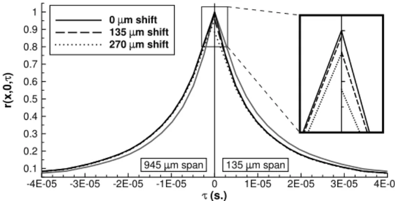
The increase of the integral timescale could nonethless be partly induced by such biases, such as, for instance, an imperfect superposition of the laser light sheets illuminating the PIV field of view. The alteration of the auto-correlation coefficients induced by such an error of superposition have been evaluated using the LES database by comparing the true auto-correlation obtained from a sensor at a given location with the cross-correlation between this sensor and another one shifted in the spanwise direction. Assuming that the laser sheets of each of the independent PIV systems are perfectly aligned, the effect of spanwise shift between the two laser sheet-planes of the two PIV systems in Dual–PIV was assessed. Two separation distances exceeding the estimated maximally occurring shift have been tested. It is seen from Fig. 11 that an error in the superposition of the laser does not induce significant deviations for large time delays although
(s.) r( x ,0 , )
-4E-05 -3E-05 -2E-05 -1E-05 0 1E-05 2E-05 3E-05 4E-05 0.1 0.2 0.3 0.4 0.5 0.6 0.7 0.8 0.9 1 0 m shift 135 m shift 270 m shift 945 m span 135 m span
Figure 11. Spanwise cross-correlation coefficients computed from the LES for a two sensor spans and three
spanwise shifts. Note that the 0 µm separation data (auto-correlation coefficients) are replotted as gray lines on the other side of the y-axis for comparison purposes.
it causes a reduction in correlation level at zero time delay between the systems. This error, however, can be minimized by careful superposition of the laser light sheets prior to the experiments.
Causes inherent to the general PIV methodology are good candidates for the delay in auto-correlation decay, since a broadening of the spatial-autocorrelation function was already observed in the PIV
measure-ments in a supersonic boundary layer of Ganapathisubramani.13 The first possibility in this domain are
discretization errors/peak locking effects in the PIV experiment.22 To check for peak locking effects,
artifi-cial spatial filtering was introduced to the numerical database. However, to obtain an effect of the observed magnitude, the spatial filtering would have to be much stronger than possible with peak locking in our ex-periment, especially for the streamwise components that were investigated here. This is thus not the (major)
source of the observed deviation. This result is also in agreement with the observations of Christensen,6who
investigated the influence of peak-locking errors on turbulence statistics and spatial correlations in detail. Another possible source is related to the inevitable integration across the width of the laser-light sheet in PIV measurements. It has been been evaluated by computing the autocorrelation from LES data averaged in the spanwise direction over a width of 945 µm being of the same order of magnitude as the thickness of the laser sheet. The left quadrant in Fig. 11 shows that the width of the spanwise-averaged auto-correlation curve is increased compared with the exact results. This indeed contributes to an overestimation of the integral time scale, but the effect is not strong enough to be the sole cause of the overestimation.
We consequently conclude from theses various tests that the large integral time scale found in the experi-ments is unlikely to be spuriously induced by our PIV / Dual–PIV methodology. It is rather a genuine feature
of the flow since it was also observed by Ganapathisubramani13when analyzing a similar flow with a different
PIV methodology within a different wind tunnel. It makes the present dual-PIV measurements an a priori reliable basis for the computation of the power spectrum through the reconstruction of the auto–correlation function.
We proceed to the power spectra computed from auto-correlations, which were reconstructed using the different methods. They are compared in Fig. 12 for different subsets of temporal delays: (a) δτ = 2, 5, 10, 20, 40, 80, 120, . . . , 400 µs, and (b) δτ = 40, 80, 120, . . . , 400 µs, respectively. The same comments are valid for experimental data and LES data. It is clear that the set of delay times defined from the LES analysis is also suitable for an appropriate reconstruction of the autocorrelation function from experimental data. From Fig. 12 it appears that adding smaller delay times (2, 5, 10, and 20 µs) modifies the spectra estimation only for the linear and spline interpolation methods.
The power spectra reconstructed from the auto-correlation estimated from PIV measurement data are compared to LES spectra in Fig. 12 for the two different subsets of temporal delays. For both subsets, the experimental spectra obtained with the cross-correlation based scheme are found to follow the LES spectra and the −5/3 power law up to frequencies of about 150 − 200 kHz, which corresponds to the estimated cut-off
frequency of the seeding particles (see Schreyer et al.26, 27), resulting in a dynamic range of more than two
decades.
The dynamic ranges achieved by the spectra computed from linear and spline interpolations of the auto-correlation are far lower. Both methods yield spectra that follow the −5/3 power law up to 80 KHz at best
f (Hz) P S Du ( A rb it ra ry s c a le ) 103 104 105 10-7 10-6 10-5 10-4 LES Exp., equation 6 f -5/3 f (Hz) P S Du ( A rb it ra ry s c a le ) 103 104 105 10-7 10-6 10-5 10-4 LES Exp., linear Exp., spline f -5/3 (a) τ = (2, 5, 10, 20, 40, 80, . . . , 400) µs. f (Hz) P S Du ( A rb it ra ry s c a le ) 103 104 105 10-7 10-6 10-5 10-4 LES Exp., equation 6 f -5/3 f (Hz) P S Du ( A rb it ra ry s c a le ) 103 104 105 10-7 10-6 10-5 10-4 LES Exp., linear Exp., spline f -5/3 (b) τ = (40, 80, . . . , 400) µs.
Figure 12. Power spectra computed from the reconstruction of the auto-correlation function based on PIV
measurements with different methods for two different selections of temporal delays. The black dashed line represents the Kolmogorov power decay of −5/3.
when the extra small delay times (2, 5, 10, and 20 µs) are taken into account. If these extra delay times are omitted, the spectra are strongly distorted through a modification of the relative weights of the low-frequency and high-low-frequency content, resulting in the disappearance of the inertial subrange. Note that the above-described difference in the integral timescales between LES and experiments induces in the spectral domain a similar though much milder distortion of the experimental, cross correlation–computed spectra with respect to the LES spectrum.
V.
Conclusions
A new technique to estimate spectra from experimental data at discrete points in time was presented and discussed. The experimental data was measured by means of a Dual–PIV system in a turbulent flat-plate boundary layer at Mach 2. The cross-correlation information in space made available by the PIV data was used to reconstruct the auto-correlation in time. This approach is applicable for convection-dominated regions of the flow by moving into the convected frame of reference, similarly to the Taylor hypothesis.
The suitability of the method was demonstrated based on LES simulations of the same flow field. The combined experimental-numerical approach offers the possibility to improve the method by testing different parameters. For example, the optimum time delays were be determined according to suggestions derived from the numerical investigation.
Different interpolation schemes were also compared. As far as boundary layer flow is concerned, the cross-correlation–based interpolation scheme is both more accurate and more robust with respect to the choice of a time–delay set than both the linear and cubic spline interpolations, while requiring a lower number of discrete time delays. Moreover, it accuracy can be estimated a priori in a rather accurate and efficient way, making easier the optimal setting of the time–delay set.
Overall, the obtained results demonstrate the applicability of the suggested method in supersonic bound-ary layer flows and encourage its application for more complex flow fields like shock wave / turbulent boundary layer interactions.
The technique thus gives access to the spectral content of complex flows based on experimental data at a limited number of discrete points in time, which allows to greatly reduce experimental effort and costs.
One may eventually note that the present system requires to rely on a continuous wind-tunnel in order to obtain converged cross-correlation data. This is only because of the very low sampling rate of the high-resolution cameras in use. However, cameras with more than twenty time higher sampling rates exist, without suffering too large reductions of their resolution. For instance, using cameras with a 100 Hz sampling rate
would require measurements for 200 s in order to sample for each of the ten distinct time delays of subset Θ4
the 2000 flow fields from which converged cross-correlation maps can be computed. The estimation of velocity spectra using the method described in this paper would consequently require only a very low number of runs in a supersonic blowdown facility.
Acknowledgments
This work received financial support by the CNES within the research program ATAC, the ANR within the program DECOMOS, and also the Labex MEC. For the LES simulations, this work was granted access to the HPC resources of IDRIS under the allocation 2014-2a1877 made by GENCI. This support is gratefully acknowledged as well as the the support of DantecDynamics during the development of the Dual–PIV system.
References
1Agostini, L., Larchevˆeque, L., Dupont, P., Debi`eve, J.-F., and Dussauge, J.-P., Zones of Influence and Shock Motion in a
Shock/Boundary-Layer Interaction, AIAA Journal, (50):1377–1387, 2012.
2Beresh S. J., Kearney, S. P., Wagner, J. L., Guildenbecher D. R., Henfling J. F., Spillers R. W., Pruett B. O. M., Jiang
N., Slipchenko M. N., Mance J., and Roy, S., Pulse-Burst PIV in a High-Speed Wind Tunnel, AIAA Paper 2015-1218, 53rd AIAA Aerospace Science Meeting, Kissimmee, Florida, 5-9 January 2015.
3Blackman, R. B., and Tukey, J. W., 1958: The measurement of power spectra from the point of view of communication
engineering. Dover Publications, New-York, 1958.
4Bridges, J., and Wernet, M., Measurements of Aeroacoustic Sound Sources in Turbulent Jets, AIAA/CEAS Aeroacoustics
Conference and Exhibit, Hilton Head, South Carolina, 12-14 May, 2003.
5Bridges, J., Effect of Heat on Space-Time Correlations in Jets, 12th AIAA/CEAS Aeroacoustics Conference, Cambridge,
Massachusetts, 8-10 May, 2006.
6Christensen, K. T., The influence of peak-locking errors on turbulence statistics computed from PIV ensembles,
Experi-ments in Fluids 36, pp. 484-497, 2004.
7Debi`eve, J.-F., and Dupont, P., Dependence between the shock and the separation bubble in a shock wave boundary layer
interaction, Shock Waves 19, pp. 499-506, 2009.
8Ducros, F., Ferrand, V., Nicoud, F., Weber, C., Darracq, D., Gacherieu, C., and Poinsot, T., Large-eddy simulation of the
shock/turbulence interaction, J. Comput. Phys., (152):517–549, 1999.
9Dupont, P., Haddad, C., Ardissone, J. P., and Debi`eve, J.-F., Space and time organization of a shock wave/turbulent
boundary layer interaction, Aerospace Science and Technology 9(7), pp. 561-572, 2005.
10Dupont, P., Haddad, C., and Debi`eve, J.-F., Space and time organization in a shock-induced separated boundary layer,
Journal of Fluid Mechanics, (559):255-277, 2006.
11Fleury, V., Bailly, C., Jondeau, E., Michard, M., and Juve, D., Space-Time Correlations in Two Subsonic Jets Using
Dual Particle Image Velocimetry Measurements, AIAA Journal 46 (10), pp. 2498-2509, 2008.
12Ganapathisubramani, B., Longmire, E. K., Marusic, I., and Pothos, S., Dual-plane PIV technique to determine the
complete velocity gradient tensor in a turbulent boundary layer, Experiments in Fluids 39 (2), pp. 222-231, 2005.
13Ganapathisubramani, B., Statistical properties of streamwise velocity in a supersonic turbulent boundary layer, Physics
of Fluids 19, 098108, 2007.
14Ganapathisubramani, B., Clemens, N. T., and Dolling, D. S., Low-frequency dynamics of shock-induced separation in a
compression ramp interaction, Journal of Fluid Mechanics 636, pp. 397-425, 2009.
15Garnier, E., Stimulated Detached Eddy Simulation of three-dimensional shock/boundary layer interaction, Shock Waves,
(19):479–486, 2009
16Guibert, P., and Lemoyne, L., Dual particle image velocimetry for transient flow field measurements, Experiments in
Fluids 33 (2), pp. 355-367, 2002.
17Hu, H., Saga, T., Kobayashi, T., Taniguchi, N., and Yasuki, M., Dualplane stereoscopic particle image velocimetry:
system set-up and its application on a lobed jet mixing flow, Experiments in Fluids 31, pp. 277-293, 2001.
18K¨ahler, C. J., and Kompenhans, J., Fundamentals of multiple plane stereo particle image velocimetry, Experiments in
Fluids 29 (1 Supplement), pp. S070-S077, 2000.
19K¨ahler, C. J., Investigation of the spatio-temporal flow structure in the buffer region of a turbulent boundary layer by
means of multiple plane stereo PIV, Experiments in Fluids 36, pp.114-130, 2004.
20Klebanoff, P. S., Characteristics of turbulence in a boundary layer with zero pressure gradient, NACA Technical Report
21Lenormand, E., Sagaut, P., Ta Phuoc, L., and Comte, P., Subgrid-scale models for Large-Eddy Simulation of compressible wall bounded flows, AIAA Journal, (38):1340–1350, 2000.
22Max, J., Methodes et techniques de traitement du signal et applications aux mesures physiques, Fourth Edition, Masson,
Paris, 1985.
23Mullin, J. A., and Dahm, W. J. A., Dual-plane stereo particle image velocimetry (DSPIV) for measuring velocity gradient
fields at intermediate and small scales of turbulent flows, Experiments in Fluids 38 (2), pp. 185-196, 2005.
24Piponniau, S., Dussauge, J.-P., Debi`eve, J.-F., and Dupont, P., A simple model for low-frequency unsteadiness in
shock-induced separation, Journal of Fluid Mechanics 629, pp. 87-108, 2009.
25Scarano, F., and Moore, P., An advection-based model to increase the temporal resolution of PIV time series, Experiments
in Fluids, 52, pp. 919-933, 2012.
26Schreyer, A.-M., Dupont, P., Debi`eve, J.-F., Jaunet, V., Lasserre, J. J., Development of a Dual–PIV system for high-speed
flow applications, 17th International Symposium on Applications of Laser Techniques to Fluid Mechanics, Lisbon, Portugal, 07-10 July, 2014.
27Schreyer, A.-M., Larchevˆeque, L., Dupont, P., Method for spectra estimation from high-speed experimental data at
discrete points in time, AIAA Paper 2015-1485, 53rd AIAA Aerospace Science Meeting, Kissimmee, Florida, 5-9 January 2015.
28Simon, F., Deck, S., Guillen, P., Sagaut, P. and Merlen, A., Numerical Simulation of the Compressible Mixing Layer Past
an Axisymmetric Trailing Edge, J. Fluid Mech., (591):215–253, 2007.
29Smits, A. J., and Dussauge J.-P., Turbulent Shear Layers in Supersonic Flow, Second Edition, Springer Science+Business
Media Inc, New York, 2006.
30Souverein, L. J., van Oudheusden, B. W., Scarano, F., and Dupont, P., Application of a dual-plane particle image
velocimetry (dual-PIV) technique for the unsteadiness characterization of a shock wave turbulent boundary layer interaction, Measurement Science and Technology 20, pp. 1-16, 2009.
31Wernet, M. P., John, W. T., Bridges, J., Dual PIV Systems for Space-Time Correlations in Hot Jets, Proceedings of the
ICIASF, G¨ettingen, Germany,August 25-29, 2003.
32Wernet, M. P., Temporally resolved PIV for space–time correlations in both cold and hot jet flows, Measurement Science