On the structure and dynamics of sheared and rotating turbulence: Anisotropy properties and geometrical scale-dependent statistics

HAL Id: hal-00566046

https://hal.archives-ouvertes.fr/hal-00566046

Submitted on 7 Jun 2012

HAL is a multi-disciplinary open access

archive for the deposit and dissemination of

sci-entific research documents, whether they are

pub-lished or not. The documents may come from

teaching and research institutions in France or

abroad, or from public or private research centers.

L’archive ouverte pluridisciplinaire HAL, est

destinée au dépôt et à la diffusion de documents

scientifiques de niveau recherche, publiés ou non,

émanant des établissements d’enseignement et de

recherche français ou étrangers, des laboratoires

publics ou privés.

On the structure and dynamics of sheared and rotating

turbulence: Anisotropy properties and geometrical

scale-dependent statistics

Frank G. Jacobitz, Kai Schneider, Wouter J.T. Bos, Marie Farge

To cite this version:

Frank G. Jacobitz, Kai Schneider, Wouter J.T. Bos, Marie Farge. On the structure and dynamics

of sheared and rotating turbulence: Anisotropy properties and geometrical scale-dependent statistics.

Physics of Fluids, American Institute of Physics, 2010, 22, pp.085101. �10.1063/1.3457167�.

�hal-00566046�

On the structure and dynamics of sheared and rotating turbulence:

Anisotropy properties and geometrical scale-dependent statistics

Frank G. Jacobitz,1,2Kai Schneider,2,3Wouter J. T. Bos,4and Marie Farge5

1

Mechanical Engineering Program, University of San Diego, San Diego, California 92110, USA

2

Laboratoire de Mécanique, Modélisation, et Procédés Propres, Centre National de la Recherche Scientifique, Aix-Marseille Université and Ecole Centrale de Marseille, 38 Rue Joliot-Curie,

13451 Marseille Cedex 20, France

3

Centre de Mathématiques et d’Informatique, Université de Provence, 39 Rue Joliot-Curie, 13453 Marseille Cedex 13, France

4

Laboratoire de Mécanique des Fluides et d’Acoustique, Centre National de la Recherche Scientifique, Ecole Centrale de Lyon, Université de Lyon, 69134 Ecully Cedex, France

5

Laboratoire de Météorologie Dynamique, Centre National de la Recherche Scientifique, Ecole Normale Supérieure, 24 Rue Lhomond, 75231 Paris Cedex 5, France

sReceived 10 July 2009; accepted 14 May 2010; published online 2 August 2010d

This study is based on a series of nine direct numerical simulations of homogeneous turbulence, in which the rotation ratio f / S of Coriolis parameter to shear rate is varied. The presence of rotation stabilizes the flow, except for a narrow range of rotation ratios 0 , f / S , 1. The main mechanism for the flow’s destabilization is an increased turbulence production due to increased anisotropy. Reynolds stress and the dissipation rate anisotropy tensors have been evaluated and provide a reference for newly defined anisotropy measures. Wavelet-based directional energies capture the properties of velocity gradients. The intermittency of the flow in different directions is quantified with scale-dependent directional flatness. Scale-dependent helicity probability distribution functions allow one to statistically characterize the geometry of the motion at different scales. Small scales are found locally to be predominantly helical, while large scales are not since they tend to two-dimensionalization for cases with growing turbulent kinetic energy. Joint probability distribution functions show that the signs of velocity helicity and vorticity helicity are strongly correlated. This indicates that vorticity helicity tends to diminish velocity helicity. © 2010 American

Institute of Physics.fdoi:10.1063/1.3457167g

I. INTRODUCTION

Rotation and shear are important features of many

geo-physical and engineering flows ssee, for example, Ref. 1d.

Direct numerical simulations with constant vertical shear S =]U1/]x2and system rotation with constant Coriolis

param-eter f = 2V are considered in this study. The rotation axis is perpendicular to the plane of shear and points in the span-wise direction x3. It is therefore parallel or antiparallel to the

mean flow vorticity. The Cartesian coordinates x =sx , y , zd =sx1, x2, x3d refer to the streamwise, vertical, and spanwise

directions, respectively. A schematic of the mean flow con-figuration is shown in Fig.1.

In the previous studies of Bradshaw2 and Tritton,3 the

effect of rotation was found to be destabilizing in the anti-parallel configuration with 0 , f / S , 1 and stabilizing other-wise. A detailed discussion of the roles of the rotation ratio

f / S and the Bradshaw number B = f / Ssf / S − 1d ssometimes called “rotational Richardson number”d can be found in

Cambon et al.4and Leblanc and Cambon.5It was found that

Bis not sufficient to characterize the dynamics of the flow.6

The neutral cases with f / S = 0spure sheard and f / S = 1 szero absolute vorticityd are described by the same Bradshaw num-ber B = 0, but their dynamics show important differences. Comprehensive investigations of this flow include the works

by Salhi and Cambon,6Brethouwer,7and Jacobitz et al.8The

studies are complementary as different techniques are em-ployed and a variety of parameter regimes are considered. Rotating sheared turbulence has also been investigated in the context of stratification and magnetohydrodynamics. Linear

theory has been used by Salhi9and Kassinos et al.10to

com-pare the effects of rotation and stratification in such flows.

Kassinos et al.11 investigated passive scalar transport in

ro-tating sheared magnetohydrodynamic turbulence. An over-view on homogeneous turbulence dynamics including shear flows can be found in a recent monograph by Sagaut and

Cambon.12

The aim of this study is an investigation of the aniso-tropy properties of homogeneous turbulence with shear and rotation. In particular, well-established anisotropy measures, such as the Reynolds stress and dissipation rate anisotropy

tensorsssee, for example, Ref.13d, are compared to

wavelet-based measures of anisotropy recently introduced by Bos

et al.14sfor a recent review of wavelet methods, see Ref.15d. Directional energies and the corresponding spatial fluctua-tions can be quantified using the orthogonal wavelet decom-position. The conventional anisotropy measures are widely used in the community and provide a reference point for the interpretation of newly defined quantities.

In addition, decompositions of the Reynolds stress aniso-tropy tensor are considered in this study. Based on the en-ergy, helicity, and polarization decomposition of the

dimensional energy spectrum tensor developed in Cambon

and Jacquin,16a decomposition of the Reynolds stress

aniso-tropy tensor into directional anisoaniso-tropy and polarization an-isotropy was introduced, first for rotating homogeneous turbulence17and then for general anisotropic turbulence.18In

Refs.19and20, Kassinos et al. proposed single-point

turbu-lence structure tensors. The structure dimensionality aniso-tropy tensor and circulicity anisoaniso-tropy tensor also decompose the Reynolds stress anisotropy tensor. The measures

devel-oped by Kassinos et al.20 and Cambon et al.18 can be

ex-pressed as linear combinations of each other.

Another goal is the study of scale-dependent statistics, such as flatness, and geometrical quantities, such as helicity probability distribution functions. Directional flatness allows one to quantify the influence of the rotation rate on the flow intermittency. Helicity measures the alignment between the velocity and vorticity vectors and thus characterizes the pres-ence or abspres-ence of helical motion. The local scale-dependent helicity has recently been analyzed for forced isotropic

tur-bulence by Yoshimatsu et al.21

In the next section, governing equations and numerical approach are introduced. Then results from a series of simu-lations of rotating and sheared homogeneous turbulence are presented including the turbulence evolution, a comparison of conventional and novel wavelet-based anisotropy mea-sures, turbulence structure tensors, and scale-dependent

geo-metrical statistics. In particular, we will assess which char-acteristics distinguish the flows in which the kinetic energy grows from those in which it decays. Finally, conclusions of the present work are given.

II. GOVERNING EQUATIONS AND NUMERICAL APPROACH

The direct numerical simulations performed here are based on the continuity equation for an incompressible fluid and the unsteady three-dimensional Navier–Stokes equation. The following equations are used to determine the fluctuat-ing velocities u =su , v , wd = su1, u2, u3d:

¹ · u = 0, s1d ]u ]t + u · ¹u + Sx2 ]u ]x1 + Su2e1+ 2V 3 u = − 1 r0 ¹ p +n¹2_{u. s2d}

Here p contains the pressure and centrifugal force,r0 is the

density,nis the kinematic viscosity, and e1is the unit vector

in the downstream direction.

In the direct numerical approach, all dynamically active scales of the velocity field are resolved. The above equations are solved in a frame of reference moving with the mean

sheared flowssee Ref. 22d. This approach allows the

appli-cation of periodic boundary conditions for the fluctuating components of the velocity field. A spectral collocation method is used for the spatial discretization and the solution is advanced in time with a fourth-order Runge–Kutta scheme. The simulations are performed on a parallel com-puter using 2563 2563 256 grid points. The simulations analyzed in this study are identical to the ones reported in Jacobitz et al.8

In the following, results of nine simulations of rotating sheared turbulence are presented and the rotation ratio f / S is varied from 210 to 10. Negative values of f / S correspond to a parallel configuration and positive values correspond to an antiparallel configuration between the system rotation and the mean flow vorticity. Isotropic turbulence fields are used to initialize all simulations. The values of the initial Taylor

microscale Reynolds number Rel= 45 and the initial shear

number SK /e= 2 are identical for all cases. The evolution of

the Taylor microscale Reynolds number depends on the fate

of the turbulence and reaches values as high as Rel= 120.

The shear number varies only weakly with f / S and assumes

a value of about SK /e= 6 in the simulations. This suggests

TABLE I. Properties of the simulations at nondimensional time St= 5.

Case Configuration Rel SK /e g Fate

f / S= −5 Parallel 37.22 5.846 20.2176 Decay

f / S= −0.5 Parallel 42.52 4.094 20.1406 Decay

f / S= 0 Shear only 72.15 4.817 0.1338 Growth

f / S= +0.5 Antiparallel 100.43 6.036 0.3523 Growth f / S= +5 Antiparallel 35.49 5.901 20.2161 Decay

f

x

x

x

1

2

3

1

U

FIG. 1. Schematic of the mean flow configuration with uniform vertical shear S =]U1/]x2 and rotation f = 2 V. Note that this schematic shows a

that shear has a more direct influence on the time scale of the overturning turbulent eddies as compared to rotation. Typical

flow parameters are summarized in TableIfor five selected

cases taken at nondimensional time St = 5.

III. RESULTS

In this section, the turbulence evolution is first discussed. Then, the anisotropy properties of the turbulence are charac-terized using well-established measures in order to provide a reference point for the interpretation of newly defined quan-tities. Turbulence structure anisotropy tensors are discussed. Wavelet-based measures are used to obtain further informa-tion about the anisotropy properties of homogeneous turbu-lence with mean shear and system rotation. Finally, scale-dependent statistics are used to quantify the intermittency and to obtain insight into geometrical features of the flow.

A. Turbulence evolution

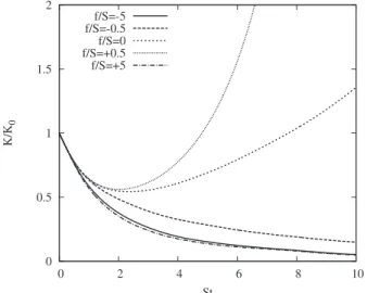
Figure 2 shows the evolution of the turbulent kinetic

energy K for a series of simulations in which the rotation ratio f / S is varied. Due to the isotropic initial conditions, the turbulent kinetic energy first decays in order to adjust to the flow anisotropy. The nonrotating case with f / S = 0 shows eventual exponential growth of K. For moderate rotation ra-tios, the antiparallel case with f / S = +0.5 leads to a strong growth of the turbulent kinetic energy, while the parallel case with f / S = −0.5 results in a decay of K. For strong rotation ratios, however, both the antiparallel case with f / S = +5 and the parallel case with f / S = −5 lead to a strong decay of K due to the importance of linear effects. These observations

are in agreement with previous resultssRefs. 2–4 and7d. A

first rough classification of the different flows can thus be made by separating flows in which the energy eventually increases from flows in which the energy decays. One of the main goals of this paper is to see whether this can be related to other features of the flow.

A first step is to separately investigate the contributions

of production and dissipation in the transport equation for the turbulent kinetic energy. This equation can be written in the following nondimensional form:

g= 1 SK dK dt = P SK− e SK. s3d

Here g is the growth rate of the turbulent kinetic energy,

P / SK is the normalized production rate, and e/_{SK is the} normalized dissipation rate. The dependence of the turbu-lence growth rategon the rotation ratio f / S is shown in Fig.

3 at nondimensional time St = 5 ssee also TableId. Positive

values ofgcorrespond to growth of turbulent kinetic energy

Kand negative values ofgcorrespond to its decay. In

accor-dance with the previous works,2–4,7the antiparallel configu-ration with 0 , f / S , 1 results in a destabilization of the flow, while other parameter ranges of the rotation ratio lead to a stabilization of the turbulence level. Both normalized

pro-duction P / SK and normalized dissipatione/SKcontribute to

the growth rateg. While the normalized dissipation rate

re-mains relatively unaffected by a variation of the rotation ra-tio, the normalized production rate strongly increases in the antiparallel case with 0 , f / S , 1, which leads to a fast growth of the turbulence. The mechanism that is responsible for the turbulent kinetic energy growth mainly acts at the large scales. We will come back to this issue in Secs. III D and III E, where we will analyze the flows using scale de-pendent statistics.

In order to investigate the effect of shear and rotation on the structure of turbulent flows, volume visualizations of the

magnitude of fluctuating vorticity are consideredsfor details

on volume visualization, see Ref.23d. Figures4and5 show

vortical structures for two cases with f / S = +0.5 and f / S = +5, respectively, at nondimensional time St = 5. In the fol-lowing, we will often take these two cases as representative for the two distinct energy evolution regimes. The vortical structures are inclined in the vertical direction relative to the

downstream direction by an anglea. This angle is larger for

the strongly growing case with f / S = +0.5 compared to the

0 0.5 1 1.5 2 0 2 4 6 8 10 K/K 0 St f/S=-5 f/S=-0.5 f/S=0 f/S=+0.5 f/S=+5

FIG. 2. Evolution of the turbulent kinetic energy K in nondimensional time

Stfor different rotation ratios f / S.

-0.4 -0.2 0 0.2 0.4 0.6 -10 -5 0 5 10 f/S γ P/SK -ε/SK

FIG. 3. Dependence of the growth rateg, normalized production P / SK, and normalized dissipation e/_SK on the rotation ratio f / S at nondimensional time St = 5.

decaying case with f / S = +5. The inclination angleaof vor-tical structures directly influences the strength of turbulence growth or decay. In the decaying case with f / S = +5, the vor-tical structures are patchy and somewhat resemble structures found in stratified flows. The flow seems to be close to a two-component flow, such as in stably stratified turbulence,

rather than to a two-dimensional flow.24 Using rapid

distor-tion theory, Salhi9 pointed out similarities between rotation

and stratification effects in homogeneous shear flow.

Simi-larly, Kassinos et al.10 provided some insight into the

inter-play of rotation and stratification. In the case f / S = +0.5, the aligned structures are more elongated, indicating a partial two-dimensionalization of the flow. A more detailed

discus-sion of the inclination angle a can be found in Jacobitz

et al.8

B. Conventional anisotropy measures

Two conventional measures for the anisotropy properties of turbulent flow are computed from the direct numerical

simulation data. The Reynolds stress anisotropy tensor bij

describes the large scale anisotropy properties

b_ij=uiuj

2K −

1

3dij. s4d

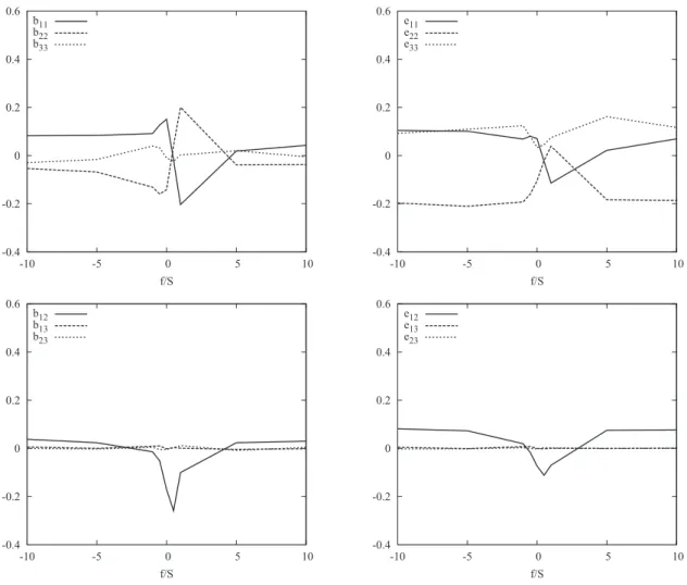
The top left part of Fig. 6 shows the dependence of the

diagonal components of the Reynolds shear stress anisotropy

tensor bij on the rotation ratio f / S at nondimensional time

St= 5. The diagonal components of bijcorrespond to the

dis-tribution of energy among the velocity components. For most rotation ratios, an ordering b11. b33. b22, i.e., streamwise

. spanwise. vertical, is observed. Only in the antiparallel

cases with 0 , f / S , 1 this ordering is changed into b22

. b33. b11, i.e., vertical. spanwise. streamwise. The

off-diagonal components of bijare shown at the bottom left part

of Fig.6. Due to the symmetry of the flow, the components

b₁₃ and b23 remain small. The magnitude of the component

b₁₂ is largest for f / S = +0.5, corresponding to the strongest growth of the turbulent kinetic energy K. Note that the nor-malized turbulence production rate is related to the aniso-tropy features of the flow since P / SK = −2b12.

The dissipation rate anisotropy tensor eijis defined in a

similar manner to describe the small scale anisotropy prop-erties of the flow

eij= n]ui ]xk ]uj ]xk 2e − 1 3dij. s5d

The top right part of Fig. 6 shows the dependence of the

diagonal components of the dissipation rate anisotropy tensor

eij on the rotation ratio f / S at nondimensional time St = 5.

Both the streamwise e11 and spanwise e33 components for

most cases show a surplus, while the vertical component e22

shows a deficit. Only in the strongly growing case with ro-tation ratio f / S = 0.5, the ordering is altered. The off-diagonal

components of eijare shown at the bottom right part of Fig.

6. Again, only the e12 component is nonzero. Overall, the

components of the dissipation rate anisotropy tensor eij

closely follow the components of the Reynolds stress

aniso-tropy tensor bij. The main drawback of the dissipation rate

anisotropy tensor is the summation over all three gradients of velocity in each component. It is therefore not possible to capture additional directional information about this flow not already described in the Reynolds stress anisotropy tensor.

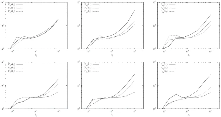
In order to gain more understanding about directional information contained in the velocity gradients, the contribu-tion of each gradient to the overall dissipacontribu-tion rate is consid-ered ei,j= n]ui ]xj ]ui ]xj 2e . s6d

In contrast to the dissipation rate anisotropy tensor, this al-ternative quantity does not require any summation over the spatial derivatives of the velocity components. The top row

in Fig. 9 shows the dependence ofei,j on the rotation ratio

f / Sat nondimensional time St = 5. The left figure shows the

three gradients of the streamwise velocity component e1,j.

For most values of the rotation ratio, the vertical component

x₃

x₂

x₁

FIG. 4.sColor onlined Volume visualization of isovorticity for f / S = +0.5 at nondimensional time St = 5. Orientation as in Fig.1.

x₃

x2

x₁

FIG. 5. sColor onlined Volume visualization of isovorticity for f / S = +5 at nondimensional time St = 5. Orientation as in Fig.1.

is the largest. It is, however, strongly reduced for the strongly growing cases with 0 , f / S , 1, where the spanwise compo-nent becomes important. The center figure shows the gradi-ents of the vertical velocity componente2,j. Again, the

span-wise gradient is strongly increased for the cases with strongly growing turbulent kinetic energy. The right figure

shows the gradients of the spanwise velocity componente3,j.

For most cases, the vertical gradient shows the largest con-tribution, but it is reduced for the cases with strongly grow-ing turbulent kinetic energy. In general, by magnitude large rotation ratios lead to large spanwise gradients of the veloc-ity components. The cases with growing turbulent kinetic energy, however, are characterized by strong vertical gradi-ents of the velocity compongradi-ents.

C. Turbulence structure anisotropy tensors

In order to gain a more complete description of the struc-ture of turbulence, we consider decompositions of the Rey-nolds stress anisotropy tensor. For homogeneous turbulence,

following Kassinos et al.,20the structure dimensionality

ten-sor Dijcan be determined from the velocity spectrum tensor

Eijskd = uˆiuˆjp, Dij=

E

Here, a hat denotes the Fourier transform, a star the complex conjugate, and k =sk1, k2, k3d is the wave vector. The

struc-ture dimensionality anisotropy tensor is then defined as follows: dij= Dij Dkk −1 3dij. s8d

Another measure introduced by Kassinos et al.20 is the

cir-culicity tensor

F_ij=

E

p k2 d

3_{k. s9d}

Here,v_{= = 3 u =sv1,v2,v3d is the vorticity vector and k is} the magnitude of the wave vector. The circulicity anisotropy tensor is then defined as follows:

-0.4 -0.2 0 0.2 0.4 0.6 -10 -5 0 5 10 f/S b11 b₂₂ b₃₃ -0.4 -0.2 0 0.2 0.4 0.6 -10 -5 0 5 10 f/S e11 e₂₂ e₃₃ -0.4 -0.2 0 0.2 0.4 0.6 -10 -5 0 5 10 f/S b₁₂ b13 b₂₃ -0.4 -0.2 0 0.2 0.4 0.6 -10 -5 0 5 10 f/S e₁₂ e13 e₂₃

FIG. 6. Dependence of the diagonal componentsstop rowd and off-diagonal components sbottom rowd of the Reynolds stress anisotropy tensor bijsleft

fij=

Fij

Fkk

−1

3dij. s10d

The Reynolds stress anisotropy tensor, structure dimension-ality anisotropy tensor, and circulicity anisotropy tensors are related,

bij+ dij+ fij= 0. s11d

Note that the circulicity anisotropy tensor is therefore deter-mined by the Reynolds stress anisotropy tensor and the di-mensionality anisotropy tensor.

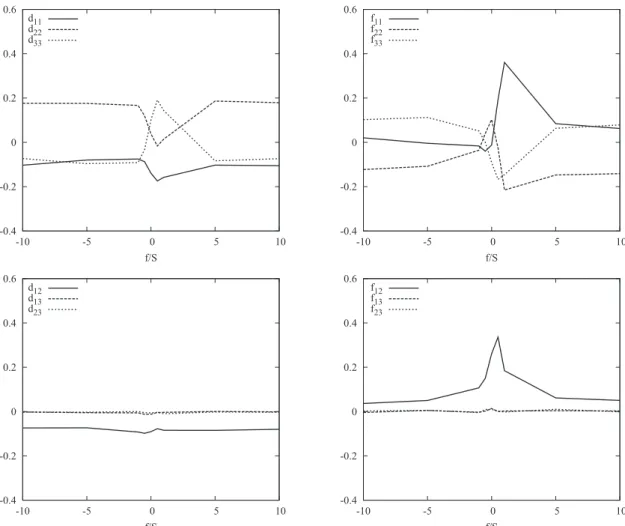
The left column of Fig.7 shows the diagonalstopd and

off-diagonal sbottomd components of the structure

dimen-sionality anisotropy tensor. For the case of homogeneous shear flow with f / S = 0, our results are consistent with those

reported by Kassinos et al.20 In this case, we observe that

d22< d33. d11, which, according to Kassinos et al.,

20

sug-gests that “the dimensionality is close to being axisymmetric

about the x1-axis.” For f / S = +0.5, an ordering d33. d22

. d11is obtained. Otherwise, we observe d11< d33, d22. For

the off-diagonal components, we observe that d13 and d23

vanish, while the component d12 assumes a value of about

20.08, independent of the rotation ratio f / S. This value

again is in agreement with Kassinos et al.20

The right column of Fig.7shows the diagonalstopd and

off-diagonal sbottomd components of the circulicity

aniso-tropy tensor, which “describes the large-scale structure of the vorticity field.”20The nonzero values of f12confirm that the

flow structures are inclined to the streamwise direction. For

growing turbulent kinetic energy, f11is the dominant

compo-nent. For negative f / S, we find f33. f11. f22 and for f / S

. 5, we observe f11< f33. f22.

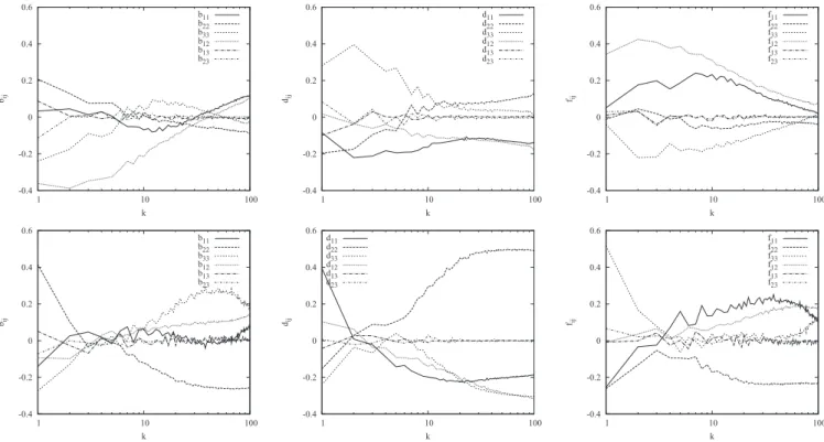
The corresponding wavenumber-dependent quantities can be defined by shell averaging in Fourier space and yield insight into the wavenumber distribution of different

aniso-tropy tensors. Figure 8 shows the wavenumber-dependent

components of the Reynolds stress anisotropy tensor bijsleft

columnd, the structure dimensionality tensor dij scenter

col-umnd, and the circulicity anisotropy tensor fijsright columnd

for two values of the rotation ratios f / S = +0.5stop rowd and

f / S= +5 sbottom rowd at nondimensional time St= 5. Those two cases were chosen to illustrate both energy-growing and energy-decaying cases. The main conclusion inspecting these plots is that the flows show no return to isotropy at large wavenumber for all quantities and all flows. In addition, we find a pronounced anisotropy at small wavenumbers and a strong dependence of the values of the turbulence structure

-0.4 -0.2 0 0.2 0.4 0.6 -10 -5 0 5 10 f/S d11 d₂₂ d₃₃ -0.4 -0.2 0 0.2 0.4 0.6 -10 -5 0 5 10 f/S f11 f₂₂ f₃₃ -0.4 -0.2 0 0.2 0.4 0.6 -10 -5 0 5 10 f/S d₁₂ d13 d₂₃ -0.4 -0.2 0 0.2 0.4 0.6 -10 -5 0 5 10 f/S f₁₂ f13 f₂₃

FIG. 7. Dependence of the diagonal componentsstop rowd and off-diagonal components sbottom rowd of the structure dimensionality anisotropy tensor dij

anisotropy tensors on the wavenumber. It remains to be veri-fied if return to isotropy is observed at higher Reynolds numbers.

Based on an energy, polarization, and helicity

decompo-sition of the three-dimensional energy spectrum tensor Eij,

Cambon et al.18suggested a decomposition of the Reynolds

stress anisotropy tensor bij into directional anisotropy bij

sed

and polarization anisotropy b_ijszd,

bij= bij

sed

+ bij

szd

. s12d

The structure dimensionality anisotropy tensor dij and the

circulicity anisotropy tensor fij can be obtained as a linear

combination of b_ijsedand b_ijszd,

dij= − 2bij sed , fij= bij sed − bij szd . s13d

The authors18showed that the directional anisotropy tensor is

correctly determined by linear theory.

D. Wavelet-based anisotropy measures

Space-scale decomposition of the flow is obtained by applying the orthogonal wavelet transform to the velocity field. Therefore, the velocity field u =su1, u2, u3d at a given

time instant is developed into an orthogonal wavelet basis

using Coiflet 12 wavelets.25 Note that the same

decomposi-tion can be applied to the vorticity field v_{= ¹ 3 u}

=sv1,v2,v3d. The projection of one component uasxd can be

represented by

uasxd =

o

u

˜_lac_lsxd, s14d

with the subscript l =sj , i , dd, where j represents the scale index, i the position, and d the direction. The orthogonal wavelet coefficients are given by u˜_la=kua,cll, where k , l

de-notes the L2_{-inner product. The wavelet coefficients measure}

the fluctuations of uaat scale 2−jand around position i / 2jfor

each of the seven possible directions d. The contribution of

the velocity component ua at scale 2−j and direction d is

obtained by fixing j and d and summing only over i in Eq. s14dand it is denoted by ua

j,d

. Its contribution ua

j

at scale 2−j

is obtained by summation over i and d in Eq. s14d while

fixing j.

Parseval’s identity allows one to obtain directional

en-ergy contributions as functions of scale j.14 For the

direc-tional scale-dependent energy distribution of a velocity

com-ponent ua, we thus obtain

E_aj,d=1₂kua

j,d

,ua

j,d

l. s15d

Summing over all scales, we get the directional energy of the

velocity component ua in the direction d,

E_ad=

o

j

E_aj,d. s16d

By construction, we obtain the total kinetic energy as follows: -0.4 -0.2 0 0.2 0.4 0.6 1 10 100 bij k b11 b22 b33 b12 b13 b23 -0.4 -0.2 0 0.2 0.4 0.6 1 10 100 dij k d11 d22 d33 d12 d13 d23 -0.4 -0.2 0 0.2 0.4 0.6 1 10 100 fij k f11 f22 f33 f12 f13 f23 -0.4 -0.2 0 0.2 0.4 0.6 1 10 100 bij k b11 b22 b33 b12 b13 b23 -0.4 -0.2 0 0.2 0.4 0.6 1 10 100 dij k d11 d22 d33 d12 d13 d23 -0.4 -0.2 0 0.2 0.4 0.6 1 10 100 fij k f11 f22 f33 f12 f13 f23

FIG. 8. Wavenumber dependence components of the Reynolds stress anisotropy tensor bijsleft columnd, structure dimensionality anisotropy tensor dijscenter

columnd, and circulicity anisotropy tensor fijsright columnd for two cases with f / S = +0.5 stop rowd and f / S = +5 sbottom rowd at nondimensional time

E=

o

j,d,a

E_aj,d=

o

d,a

E_ad. s17d

The bottom row in Fig. 9 shows the normalized directional

energy components E_ad/E for the x, y, and z components.

These wavelet-based measures exhibit a striking similarity with the normalized directional dissipation rate components

e_i,j/e. This is due to the fact that wavelet coefficients of velocity are related to its gradients and discriminate the fluc-tuations of velocity components between the seven possible directions.

Figures 10 and 11 show the directional energy of the

flow for two cases with f / S = +0.5 and f / S = +5, respectively, at nondimensional time St = 5. For the strongly growing case with f / S = +0.5, the vertical velocitysvd in the spanwise

di-rection szd contains most of the energy, followed by the

downstream velocity sud in the spanwise direction szd. For

the strongly decaying case with f / S = +5, however, the

span-wiseswd and downstream sud velocities in the vertical

direc-tion syd contain most of the energy, while vertical velocity

svd is reduced. The figures also show that the mixed

direc-tions sxy, xz, yz, and xyzd are less significant. A finer

reso-lution of the anisotropy measures would require the use of the continuous wavelet transform, which necessitates

sub-stantially more computational resources for

three-dimensional turbulence. Details on this technique applied to two-dimensional cuts of three-dimensional turbulent flows

can be found in Ruppert-Felsot et al.26

To study higher-order scale-dependent statistics, we

de-0 0.1 0.2 0.3 0.4 0.5 -10 -5 0 5 10 f/S ε_1,1 ε 1,2 ε_1,3 0 0.1 0.2 0.3 0.4 0.5 -10 -5 0 5 10 f/S ε_2,1 ε 2,2 ε_2,3 0 0.1 0.2 0.3 0.4 0.5 -10 -5 0 5 10 f/S ε_3,1 ε 3,2 ε_3,3 0 0.05 0.1 0.15 0.2 0.25 0.3 -10 -5 0 5 10 f/S E11/E E2₁/E E3₁/E 0 0.05 0.1 0.15 0.2 0.25 0.3 -10 -5 0 5 10 f/S E12/E E2₂/E E3₂/E 0 0.05 0.1 0.15 0.2 0.25 0.3 -10 -5 0 5 10 f/S E13/E E2₃/E E3₃/E

FIG. 9. Dependence of the dissipation rate componentea,bforb= 1 , 2 and 3stop rowd and directional energy component Ea

d_/

Efor d = 1 , 2, and 3sbottom rowd on the rotation ratio f / S at nondimensional time St = 5. The x1-componentsleft columnd, x2-componentscenter columnd, and x3-componentsright columnd are

shown. 0 5 10 15 20 25 xyz yz xz xy z y x % of Energy Directions u v w

FIG. 10.sColor onlined Wavelet-based directional energy for f / S = +0.5 at nondimensional time St = 5. 0 5 10 15 20 25 xyz yz xz xy z y x % o f Energy Directions u v w

FIG. 11. sColor onlined Wavelet-based directional energy for f / S = +5 at nondimensional time St = 5.

fine the p-th order centered moments of each component ua

of the vector field u at scale j from its wavelet coefficients sRef.27d M_pa_,j= 1 7 3 23j

o

o

o

o

denotes the mean value of the moment at scale j. The

scale-dependent flatness of a velocity component ua is defined as

follows: F_ja= M4,j a _/ sM2,j a d2 . s20d

It is closely related to the standard deviation of the spectral distribution of energy, which illustrates that Fj

,

yields a mea-sure of the relative spatial fluctuations of the spectral energy density.14

The scale index j is related to a wavenumber kjby the

following relationship:

kj= k02j. s21d

Here, k0is the centroid wavenumber of the mother wavelet,

which is constant for each type of wavelet, e.g., k0< 0.77 for

the Coiflet 12 used here. Wavelets have a constant relative bandwidth, which means that with increasing j, the spectral

support of the wavelet increases, and thus the spectral selec-tivity of the wavelet decreases. The scale-dependent distribu-tions of energy or flatness can be related to wavenumber distributions, in particular, to energy spectra.25

The directional scale-dependent flatness of the three

ve-locity components is shown in Fig.12. Here, we focus only

on two cases, one for f / S = +0.5 stop rowd, which is

repre-sentative of a flow with strongly growing turbulent kinetic

energy, and one for f / S = +5sbottom rowd, which represents

cases with decaying turbulent kinetic energy. A general ob-servation is a strong increase of the flatness with wavenum-ber, which reflects the flow intermittency. The intermittency here is related to the dissipation range28and the resolution of the simulations does not allow to observe a possible inertial

range intermittency. In Ref.14, it was shown that an

aniso-tropy of the small spatial scales can cause an anisoaniso-tropy of the directional flatness which is increased in certain direc-tions due to the depletion of energy, affecting particular re-gions in Fourier space. Here, it is also observed that the small-scale intermittency is anisotropic. The growth of flat-ness of all velocity components is the strongest in the streamwise direction, except for the case f / S = +0.5 where

the flatness of the u1 velocity component behaves similarly

in all directions due to the strong shear production. At mod-erate wavenumbers 2 # k # 10, a flatness value around 3 is obtained in all cases, indicating a Gaussian-like behavior. Even though the flatness is slightly different for the two cases, it does not seem straightforward to relate the large-scale production of kinetic energy directly to the directional intermittency of the flow.

100 101 102 100 101 102 kj Fu1(k1) F_u 1(k2) Fu1(k3) 100 101 102 100 101 102 kj Fu2(k1) F_u 2(k2) Fu2(k3) 100 101 102 100 101 102 kj Fu3(k1) F_u 3(k2) Fu3(k3) 100 101 102 100 101 102 k_j Fu1(k1) Fu1(k2) F_u 1(k3) 100 101 102 100 101 102 k_j Fu2(k1) Fu2(k2) F_u 2(k3) 100 101 102 100 101 102 k_j Fu3(k1) Fu3(k2) F_u 3(k3)

FIG. 12. Directional scale-dependent flatness for f / S = +0.5stop rowd and f / S = +5 sbottom rowd. The u1-componentsleft columnd, u2-componentscenter

E. Wavelet-based scale-dependent geometrical measures

Additional geometrical information about the flow can

be obtained from the velocity helicity Huand vorticity

helic-ity Hv,

Hu= u ·s¹ 3 ud, Hv=v·s¹ 3vd. s22d

After averaging over space, both quantities can be related by the helicity transport equation dkHul / dt = −2nkHvl + 2kFl.

The term F = f ·v _{accounts for any forcing terms f in the}

momentum equation, and it vanishes for linear effects, such as shear and rotation. A corresponding evolution equation for three-dimensional helicity spectrum was first given in

Cam-bon and Jacquin.16 This equation also includes a transfer

term, describing redistribution of helicity, determined by triple correlations. As in the case of the turbulent kinetic energy equation, the transfer term vanishes after averaging.

The present flow initially does not contain mean helicity and it will thus remain free from it. However, this does not concern the local helicity and regions with strong helicity can exist in a flow free from mean helicity. In the following, we will concentrate on this local helicity and its statistics.

The relative helicities of velocity and vorticity measure the cosine of the angle between the two vector quantities and are defined as follows:

hu=

u ·s¹ 3 ud

iuii¹ 3 ui, hv=

v_{·s¹ 3}v_d

iv_{ii¹ 3}v_i. s23d

The relative velocity helicity hu allows one to distinguish

between helical structuressswirling motiond and nonhelical

structures. For helical structures, huhas values of 61, which

correspond to alignment or antialignment of vorticity and

velocity, respectively. For nonhelical structures,

two-dimensionalization of the flow occurs, vorticity is

perpen-dicular to velocity, and the velocity helicity hu assumes a

value hu= 0. Using the vector identity = 3v= −Du, the

rela-tive vorticity helicity hv measures the cosine of the angle

between vorticity and the negative Laplacian of velocity,

which is related to dissipation. The velocity helicity hu and

vorticity helicity hvcan also be interpreted as the correlation

coefficients between u with v _and v _{with = 3}v_,

respec-tively.

Scale-dependent helicities huj and h_vjcan be defined by

replacing u andv_{in Eq.s23dby u}j_andvj_{, respectively, as}

recently introduced in Ref. 21. Thus, geometrical statistics

can be obtained at different scales of the flow.

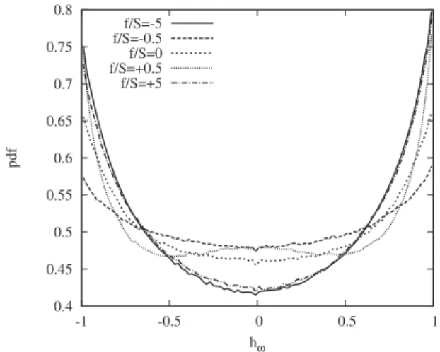
Figures13and14show the probability distribution

func-tionssPDFsd of the relative helicities of velocity and

vortic-ity, respectively. The PDFs of hu show a maximum for hu

= 0 for cases with growing turbulent kinetic energy sf / S = 0

and f / S = +0.5d, indicating a higher probability for two-dimensional motion. For decaying cases, a maximum for

hu6 1 is observed, corresponding to a higher probability for

helical motion. The PDFs of hvshow a maximum for hv6 1

for all cases and the alignment or antialignment of vorticity with the negative Laplacian of velocity is particularly pro-nounced in the case of strong rotationsf / S = 6 5d.

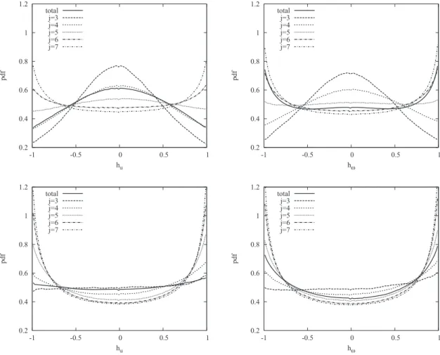
Figure 15 shows the scale-dependent velocity helicity

PDFsleft columnd and vorticity helicity PDF sright columnd

for cases with f / S = +0.5stop rowd and f / S = +5 sbottom rowd at nondimensional time St = 5. The scale-dependent velocity helicity PDFs confirm the significant difference between the two cases f / S = +0.5 and +5, representing turbulence growth and decay, respectively, that we have mentioned above. For the former case, the PDFs show a pronounced

two-dimensional behavior at large scales sj = 3 , 4 , 5d, while for

the latter no peak around huj= 0 can be observed. The

prob-ability to have swirling motion at small scales is also more pronounced for f / S = +5. Similar conclusions hold for the scale-dependent distributions of vorticity helicity. These re-sults clearly show that the mechanism which distinguishes the cases f / S = +0.5 and +5 is related to the large scales, as we have conjectured in Sec. III A. Apparently, in the f / S = +0.5 case, the large scale flow shares some features with two-dimensional turbulence and the energy cascade is thus less efficient in transporting energy toward the small scales compared to three-dimensional turbulence.

Sanada29conjectured thatkHul and kHvl have a tendency

to have the same sign. This tendency also holds for the

cor-responding pointwise quantities Hu and HvsRef.30d. If this

conjecture holds, Hvacts as a “kind of viscous dissipation”

0.25 0.3 0.35 0.4 0.45 0.5 0.55 0.6 0.65 -1 -0.5 0 0.5 1 pdf h_u f/S=-5 f/S=-0.5 f/S=0 f/S=+0.5 f/S=+5

FIG. 13. Velocity helicity distribution huat nondimensional time St = 5.

0.4 0.45 0.5 0.55 0.6 0.65 0.7 0.75 0.8 -1 -0.5 0 0.5 1 pdf hω f/S=-5 f/S=-0.5 f/S=0 f/S=+0.5 f/S=+5

for Hu, independent of its sign. To verify Sanada’s conjecture

that both velocity helicity and vorticity helicity have the

same sign, we show in Fig.16the joint probability

distribu-tion funcdistribu-tion pshu, hvd. For all flows, the joint PDFs of hu

and hv are not statistically independent. We find a higher

probability in the two quadrants in which huand hvhave the

same sign as in those with opposite signs. The highest prob-ability is observed in lower left and upper right corners, cor-responding to a high probability to find alignment or

anti-alignment of u with v _and v _{with = 3v. This result}

supports the conjecture reported by Sanada29and Galanti and

Tsinober.30For comparison, we also added the joint PDF for

independently uniformly distributed velocity helicity and vorticity helicity fields, which results in a uniform joint PDF with mean value 1/4.

IV. CONCLUSIONS

Nine direct numerical simulations of homogeneous tur-bulence with shear and rotation have been performed and analyzed for this study. The turbulent kinetic energy was found to grow strongly in the antiparallel configuration with 0 , f / S , 1 and to decay otherwise. The growth is due to an

increased normalized turbulence production P / SK = −2b12

that is directly related to the only nonzero off-diagonal com-ponent of the Reynolds stress anisotropy tensor. It was also

observed that the growth rate of the turbulence is related to the inclination angle of vortical structures relative to the

downstream direction.8

The anisotropy of the flows is investigated with conven-tional measures, such as the Reynolds stress anisotropy ten-sor, the dissipation rate anisotropy tenten-sor, and the normalized components of the dissipation rate. In addition, turbulence structure anisotropy tensors are considered and results for

sheared turbulence are in agreement with Kassinos et al.20

The wavenumber-dependent tensors showed no return to isotropy at large wavenumbers. The directional energy of the flow, obtained from orthogonal wavelet decomposition of the velocity field, allows one to give an alternative measure of the anisotropy of the flow. Wavelets, such as structure func-tions, are sensitive to velocity differences in the different directions and allow to characterize streamwise, vertical, and spanwise anisotropy. Furthermore, orthogonal wavelets have the advantage that, due to their orthogonality, the energies contained in the different directions sum up to the total en-ergy, unlike structure functions or one-dimensional spectra. It has been shown in this paper that these directional energies capture the properties of velocity gradients in rotating shear turbulence. For the strongly growing case with f / S = +0.5, the spanwise differences of vertical velocity contain most of the energy, followed by the spanwise differences of down-stream velocity. For the strongly decaying case with f / S

0.2 0.4 0.6 0.8 1 1.2 -1 -0.5 0 0.5 1 pdf h_u total j=3 j=4 j=5 j=6 j=7 0.2 0.4 0.6 0.8 1 1.2 -1 -0.5 0 0.5 1 pdf hω total j=3 j=4 j=5 j=6 j=7 0.2 0.4 0.6 0.8 1 1.2 -1 -0.5 0 0.5 1 pdf h_u total j=3 j=4 j=5 j=6 j=7 0.2 0.4 0.6 0.8 1 1.2 -1 -0.5 0 0.5 1 pdf hω total j=3 j=4 j=5 j=6 j=7

FIG. 15. Scale-dependent velocity helicity distribution hujsleft columnd and vorticity helicity distribution h_vjsright columnd for f / S = +0.5 stop rowd and for

= +5, however, the vertical differences of spanwise and downstream velocities contain most of the energy, while ver-tical velocity is strongly reduced. It has thus been confirmed that wavelet-based directional energy measures agree with conventional measures.

The intermittency of the different flows studied here has been quantified using scale-dependent flatness in the differ-ent flow directions. Small-scale intermittency has been ob-served in most cases with an increased level of intermittency in the streamwise direction. At intermediate scales, a Gaussian-like behavior has been found. These observations confirm that the scale-dependent flatness is well suited to quantify the flow intermittency in different directions.

The geometrical statistics of the flows have been ana-lyzed by considering PDFs of velocity helicity and of vortic-ity helicvortic-ity. For the cases with growing turbulent kinetic en-ergy, the local relative helicity indicates a tendency toward two-dimensional motion. However, for the decaying cases,

helical motionsreflected by an alignment or antialignment of

velocity and vorticityd is mainly observed. A scale-dependent study of helicity shows that for all cases small scales exhibit helical motion, while two-dimensionalization is observed at larger scales. It has thus been shown that the helicity of the flow strongly depends on the scale.

Joint PDFs of velocity helicity and vorticity helicity in-dicate a strong correlation of the signs of these quantities. This observation supports the conjectures reported by

Sanada29and Galanti and Tsinober.30The results suggest that

vorticity helicity tends to diminish velocity helicity for rotat-ing and sheared turbulence.

ACKNOWLEDGMENTS

F.G.J. acknowledges support from the Ecole Centrale de Marseille, the Université de Provence, and an International Opportunity Grant from the University of San Diego. W.B., M.F., and K.S. acknowledge financial support from the ANR sProject No. M2TFPd and K.S. thanks the University of San Diego for its hospitality. M.F. is grateful to the Wissen-schaftskolleg zu Berlin for its support. We thank B. Kadoch for the preparation of the volume visualizations.

1

M. S. Miesch, “Large-scale dynamics of the convection zone and ta-chocline,” Living Rev. Solar Phys. 2, 1s2005d.

2

P. Bradshaw, “The analogy between streamline curvature and buoyancy in turbulent shear flow,”J. Fluid Mech. 36, 177s1969d.

3

D. J. Tritton, “Stabilization and destabilization of turbulent shear-flow in a rotating fluid,”J. Fluid Mech. 241, 503s1992d.

4

C. Cambon, J.-P. Benoit, L. Shao, and L. Jacquin, “Stability analysis and large-eddy simulation of rotating turbulence with organized eddies,”J. Fluid Mech. 278, 175s1994d.

5

S. Leblanc and C. Cambon, “On the three-dimensional instabilities of plane flows subjected to Coriolis force,”Phys. Fluids 9, 1307s1997d.

6

A. Salhi and C. Cambon, “An analysis of rotating shear flow using linear theory and DNS and LES results,”J. Fluid Mech. 347, 171s1997d.

7

G. Brethouwer, “The effect of rotation on rapidly sheared homogeneous turbulence and passive scalar transport. Linear theory and direct numerical simulations,”J. Fluid Mech. 542, 305s2005d.

8

F. G. Jacobitz, L. Liechtenstein, K. Schneider, and M. Farge, “On the structure and dynamics of sheared and rotating turbulence: Direct numeri-cal simulation and wavelet-based coherent vortex extraction,”Phys. Fluids

20, 045103s2008d.

9

A. Salhi, “Similarities between rotation and stratification effects on homo-geneous shear flow,”Theor. Comput. Fluid Dyn. 15, 339s2002d.

-1 -0.5 0 0.5 1 -1 -0.5 0 0.5 1 hω h_u 0 0.2 0.4 0.6 0.8 1 1.2 -1 -0.5 0 0.5 1 -1 -0.5 0 0.5 1 hω hu 0.22 0.23 0.24 0.25 0.26 0.27 0.28 -1 -0.5 0 0.5 1 -1 -0.5 0 0.5 1 hω h_u 0 0.1 0.2 0.3 0.4 0.5 0.6 0.7 0.8 0.9 1 -1 -0.5 0 0.5 1 -1 -0.5 0 0.5 1 hω hu 0 0.2 0.4 0.6 0.8 1 1.2 1.4 -1 -0.5 0 0.5 1 -1 -0.5 0 0.5 1 hω h_u 0 0.2 0.4 0.6 0.8 1 1.2 1.4 1.6 -1 -0.5 0 0.5 1 -1 -0.5 0 0.5 1 hω hu 0 0.2 0.4 0.6 0.8 1 1.2 1.4 1.6

FIG. 16.sColor onlined Joint PDFs of velocity helicity huwith vorticity helicity hvfor cases with f / S = 0stop leftd, f / S = +0.5 stop centerd, f / S = −0.5 sbottom

10

S. C. Kassinos, E. Akylas, and C. A. Langer, “Rapidly sheared homoge-neous stratified turbulence in a rotating frame,”Phys. Fluids 19, 021701

s2007d.

11

S. C. Kassinos, B. Knaepen, and D. Carati, “The transport of a passive scalar in magnetohydrodynamic turbulence subjected to mean shear and frame rotation,”Phys. Fluids 19, 015105s2007d.

12

P. Sagaut and C. Cambon, Homogeneous Turbulence Dynamics sCam-bridge University Press, CamsCam-bridge, 2008d.

13

C. G. Speziale and T. B. Gatski, “Analysis and modelling of anisotropies in the dissipation rate of turbulence,”J. Fluid Mech. 344, 155s1997d.

14

W. J. T. Bos, L. Liechtenstein, and K. Schneider, “Small scale intermit-tency in anisotropic turbulence,”Phys. Rev. E 76, 046310s2007d.

15

K. Schneider and O. Vasilyev, “Wavelet methods in computational fluid dynamics,”Annu. Rev. Fluid Mech. 42, 473s2010d.

16

C. Cambon and L. Jacquin, “Spectral approach to non-isotropic turbulence subjected to rotation,”J. Fluid Mech. 202, 295s1989d.

17

C. Cambon, L. Jacquin, and J. L. Lubrano, “Toward a new Reynolds stress model for rotating turbulent flows,”Phys. Fluids A 4, 812s1992d.

18

C. Cambon, N. N. Mansour, and F. S. Godeferd, “Energy transfer in ro-tating turbulence,”J. Fluid Mech. 337, 303s1997d.

19

S. C. Kassinos and W. C. Reynolds, “A structure-based model for the rapid distortion of homogeneous turbulence,” Stanford Report No. TF-61, 1994.

20

S. C. Kassinos, W. C. Reynolds, and M. M. Rogers, “One-point turbulence structure tensors,”J. Fluid Mech. 428, 213s2001d.

21

K. Yoshimatsu, N. Okamoto, K. Schneider, Y. Kaneda, and M. Farge,

“Intermittency and scale-dependent statistics in fully developed turbu-lence,”Phys. Rev. E 79, 026303s2009d.

22

R. S. Rogallo, “Numerical experiments in homogeneous turbulence,” NASA Report No. TM 81315, 1981.

23

J. Clyne, P. Mininni, A. Norton, and M. Rast, “Interactive desktop analysis of high resolution simulations: Application to turbulent plume dynamics and current sheet formation,”New J. Phys. 9, 301s2007d.

24

C. Cambon, “Turbulence and vortex structures in rotating and stratified flows,”Eur. J. Mech. B/Fluids 20, 489s2001d.

25

M. Farge, “Wavelet transforms and their applications to turbulence,”

Annu. Rev. Fluid Mech. 24, 395s1992d.

26

J. Ruppert-Felsot, M. Farge, and P. Petitjeans, “Wavelet tools to study intermittency: Application to vortex bursting,”J. Fluid Mech. 636, 427

s2009d.

27

K. Schneider, M. Farge, and N. Kevlahan, “Spatial intermittency in two-dimensional turbulence: A wavelet approach,” in Woods Hole

Mathemat-ics: Perspectives in Mathematics and Physics, edited by N. Tongring and R. C. PennersWorld Scientific, Singapore, 2004d, Vol. 34, p. 302.

28

R. H. Kraichnan, “Intermittency in the very small scales of turbulence,”

Phys. Fluids 10, 2080s1967d.

29

T. Sanada, “Helicity production in the transition to chaotic flow simulated by Navier–Stokes equation,”Phys. Rev. Lett. 70, 3035s1993d.

30

B. Galanti and A. Tsinober, “Physical space properties of helicity in quasi-homogeneous forced turbulence,”Phys. Lett. A 352, 141s2006d.