HAL Id: hal-00298994
https://hal.archives-ouvertes.fr/hal-00298994
Submitted on 1 Jan 2001
HAL is a multi-disciplinary open access
archive for the deposit and dissemination of
sci-entific research documents, whether they are
pub-lished or not. The documents may come from
teaching and research institutions in France or
abroad, or from public or private research centers.
L’archive ouverte pluridisciplinaire HAL, est
destinée au dépôt et à la diffusion de documents
scientifiques de niveau recherche, publiés ou non,
émanant des établissements d’enseignement et de
recherche français ou étrangers, des laboratoires
publics ou privés.
Detecting premonitory seismicity patterns based on
critical point dynamics
G. Zöller, S. Hainzl
To cite this version:
G. Zöller, S. Hainzl. Detecting premonitory seismicity patterns based on critical point dynamics.
Natural Hazards and Earth System Science, Copernicus Publications on behalf of the European
Geo-sciences Union, 2001, 1 (1/2), pp.93-98. �hal-00298994�
c
European Geophysical Society 2001
Natural Hazards
and Earth
System Sciences
Detecting premonitory seismicity patterns based on critical point
dynamics
G. Z¨oller1and S. Hainzl1,2
1Institute of Physics, University of Potsdam, Germany 2Institute of Earth Sciences, University of Potsdam, Germany
Received: 8 May 2001 – Accepted: 16 July 2001
Abstract. We test the hypothesis that critical point dynamics
precedes strong earthquakes in a region surrounding the fu-ture hypocenter. Therefore, we search systematically for re-gions obeying critical point dynamics in terms of a growing spatial correlation length (GCL). The question of whether or not these spatial patterns are correlated with future seismic-ity is crucial for the problem of predictabilseismic-ity. The analysis is conducted for earthquakes with M ≥ 6.5 in California. As a result, we observe that GCL patterns are correlated with the distribution of future seismicity. In particular, there are clear correlations in some cases, e.g. the 1989 Loma Prieta earthquake and the 1999 Hector Mine earthquake. We claim that the critical point concept can improve the seismic hazard assessment.
1 Introduction
Different critical point concepts have been discussed exten-sively with respect to the predictability of earthquakes (Bufe and Varnes, 1993; Jaum´e and Sykes, 1999; Hainzl et al., 1999, 2000; Hainzl and Z¨oller, 2001). Motivated by dam-age mechanics and laboratory experiments (Leckie and Hay-hurst, 1977; Das and Scholz, 1981), the time-to-failure ap-proaches assume that the preparatory process of a large earth-quake is characterized by a highly correlated stress field with a growing correlation length (GCL) and an accelerating en-ergy/moment (AMR) release. In practice, these concepts have been tested by fitting time-to-failure relations to seis-micity data. For the AMR model, this relation is
(6 √
E)(t ) = A − B(tf −t )m, (1)
with positive constants A, B, m, the time-to-failure tf, and the cumulative Benioff strain (6
√
E)(t ), where E is the en-ergy release of an earthquake. In the GCL model, the
corre-Correspondence to: G. Z¨oller ([email protected])
lation length ξ is expected to diverge for t → tf according to
ξ(t ) = C(tf −t )−k (2)
with positive constants C and k. Both approaches describe the same underlying mechanism, namely, the critical point dynamics. An important problem is the determination of free parameters, which are in addition to A, B, tf, and m in Eq. (1), respectively, C, tf, and k in Eq. (2), which represent windows for space, time, and magnitude.
The accelerating moment release in terms of cumulative Benioff strain has been documented in several cases, e.g. for California seismicity (Bufe and Varnes, 1993; Bowman et al., 1998; Brehm and Braile, 1998, 1999). The growth of the spatial correlation length has been concluded from varia-tions in the epicenter distribution (Z¨oller et al., 2001). How-ever, these studies have not been conducted systematically in space and time, i.e. the analysis was restricted to the oc-currence time and the epicenter of the largest events. Thus, possible false alarms (critical point behaviour without a sub-sequent strong earthquake) have not been examined. There-fore, it is an open question whether or not the observed phe-nomena are unique, i.e. the occurrence of patterns prior to large earthquakes is only meaningful if there is a system-atic correlation between these patterns and subsequent earth-quakes.
In the present work, we compare patterns based on crit-ical point dynamics in terms of GCL before strong earth-quakes with the epicenters of these events, and subsequent intermediate to large earthquakes. By performing a system-atic spatial search algorithm, we address the question of spa-tial correlations. To estimate the significance of the results, the method is also applied to catalogues from an appropriate Poisson process model.
2 Data and method
In this section, we present the data and the method to detect spatial correlations between GCL patterns and subsequent
94 G. Z¨oller and S. Hainzl: Critical point dynamics San Francisco San Diego Sacramento Los Angeles Las Vegas Carson f d a c h g i b e -124˚ W -124˚ W -122˚ W -122˚ W -120˚ W -120˚ W -118˚ W -118˚ W -116˚ W -116˚ W -114˚ W -114˚ W 32˚ N 32˚ 34˚ N 34˚ 36˚ N 36˚ 38˚ N 38˚ 40˚ N 40˚ 0 100 200
km
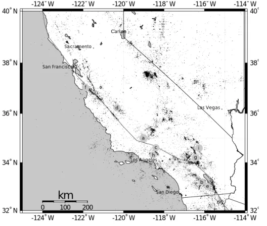
Fig. 1. Earthquakes with M ≥ 3.0 in California since 1910. Solid cir-cles denote the events with M ≥ 6.5 since 1952: circle (a), 1952 M = 7.5 Kern County; circle (b), 1968 M = 6.5 Borrego Mountain; circle (c), 1971 M =6.6 San Fernando; circle (d), 1983 M = 6.7 Coalinga; circle (e), 1987 M =6.6 Superstition Hills; circle (f), 1989 M = 7.0 Loma Prieta; circle (g), 1992 M = 7.3 Landers; circle (h), 1994 M = 6.6 Northridge; and circle (i), 1999 M = 7.1 Hector Mine.
seismicity.
We analyze the seismicity in California between the 32◦N and 40◦N latitude and the −125◦W and −114◦W longitude. The data are taken from the Council of the National Seismic System (CNSS) Worldwide Earthquake Catalogue. The cat-alogue covers the time span from 1910 to 2000. The distri-bution of earthquakes is shown in Fig. 1. To account for the completeness of the data, we restrict the analysis to the nine strongest earthquakes with M ≥ 6.5 since 1952. Note that completeness of the CNSS catalogue was not achieved until 1940.
For a detailed description of the GCL model, we refer to Z¨oller et al. (2001). The method is based on a fit of Eq. (2) to the data in a circular space window with radius R and in a time interval (t0;tf)for earthquakes with magnitudes M ≥
Mcut = 4.0. The exponent k is set to k = 0.4 according to the result of Z¨oller et al. (2001). The power law fit is then compared with the fit of a constant and the quality of the power law fit is measured by the curvature value introduced by Bowman et al. (1998),
C =power law fit root-mean-square error
constant fit root-mean-square error . (3) Around each epicenter of a strong earthquake, the curvature parameter has been calculated for different values of R and t0. The set of parameters for which C is minimal is used
for further calculations; i.e. the space window (R) and the length of the time interval (t0) are adjusted in order to
opti-mize C. The approach of looking at different spatial scales is
based on the observation of Z¨oller et al. (1998), that the dy-namics of a spatially extended system is most clearly visible on intermediate spatial scales between the noisy microscales and the large scales, where the dynamics are hidden due to the averaging. The C values are determined on a spatial grid with a resolution of 0.5◦in longitude and latitude at nine dif-ferent times tfi, corresponding to the occurrence times of the nine earthquakes with M ≥ 6.5, denoted with index i. The result is a function Ci(x) for the GCL model, which is com-pared with the epicenter distribution of the earthquakes with M ≥ 5.0 in the time interval (tfi;tfi +1 year). This set of epicenters is called the pattern Qi(x) for the ith strongest earthquake. The (arbitrary) magnitude threshold M = 5.0 defining the pattern Qi(x) has been introduced, since the premonitory patterns are assumed to be correlated not only with the strongest earthquake, but also with some subsequent main shock activity.
In the next step, the curvature parameter CiAPC(x) is calcu-lated for 100 adjusted Poisson catalogues (APC) in order to derive a measure for the statistical significance of the results. These catalogues are calculated according to the algorithm of Z¨oller et al. (2001):
1. The CNSS catalogue is declustered using the algorithm of Reasenberg (1985);
2. Random epicenters according to the epicenter distribu-tion of the declustered CNSS catalogue are calculated; 3. The earthquake occurrence times are drawn from a
4. The earthquake magnitudes are taken randomly from a probability distribution fulfilling the Gutenberg-Richter law (Gutenberg and Richter, 1956);
5. Aftershocks according to the law of Omori (1894) are added using the algorithm of Reasenberg (1985) in the inverse direction.
The resulting earthquake catalogue corresponds to a Poisson process in time with additional aftershock activity. The dis-tributions of the epicenters and the magnitudes are similar to those of the genuine catalogue. Note that only the spatiotem-poral correlations of the seismicity are randomized and all other features are preserved. Therefore, the APCs allow one to test for systematic spatiotemporal behaviour.
The likelihood ratio test has been proposed by Gross and Rundle (1998) in order to compare two models with respect to their suitability to describe an observed data set. In this work, the observed data are given by the set Qi(x) of epicen-ters with M ≥ 5.0 after the ith strongest earthquake. Model 1 is defined by the GCL pattern of the original catalogue before the ith strongest earthquake, i.e. the distribution of curvature parameters Ci(x) in space. Model 2 is the corresponding pat-tern CiAPC(x) for an APC. For both models, the likelihood function L is computed with respect to the N earthquakes, forming the pattern Qi(x):
L =
N
Y
k=1
P (xk, Ck). (4)
P (xk, Ck)is the normalized probability density for an event occurring at the epicenter xk with a premonitory GCL pat-tern characterized by the curvature parameter Ck. To ap-ply the likelihood ratio test, we assume Gaussian probabil-ity densprobabil-ity functions P (x, C) = p1(x) × p2(C) consisting
of a two-dimensional Gaussian function p1around the
spa-tial grid node x with standard deviation σ1and a (right wing)
Gaussian function p2depending on the curvature parameter
C with standard deviation σ2. The value of σ1is the distance
between two adjacent grid nodes and σ2=0.35 is an
empir-ical value (Z¨oller et al., 2001). It should be noted that Eq. (4) must be applied cautiously, since this equation only holds if the N earthquakes are statistically independent.
The likelihood function is also measured for each of the APCs (model 2). The likelihood ratio LRi =L/LAPCof the
normalized likelihood functions for model 1 and model 2 is equal to the probability ratio p/pAPC, where p denotes the
probability that Qi(x) arises from the original data (model 1) and pAPC is the corresponding probability for the APCs
(model 2). In the case of LRi > 1, the detected GCL pat-terns in the original catalogue are more correlated with the subsequent occurring intermediate to large earthquakes. In contrast, LRi <1 means that the patterns from the random catalogue are correlated with the future seismicity. Due to a rather skewed distribution of LRi, the mean value hLRiiis not an appropriate measure for the spatial correlations. In-stead, we use the number Nsi of APCs that is a better fit than the original model (LRi < 1) and represents a more robust
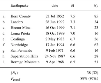
Table 1. Results of Likelihood Ratio Test. Nsis the number of ad-justed Poisson catalogues, where the GCL patterns are more corre-lated with main shock activity than for the CNSS catalogue. Pconf is the probability that nine random numbers (corresponding to the nine strong earthquakes) have a mean value smaller than or equal to hNsi. The values in the parentheses are the results for hNsiand Pconf without the Kern County earthquake
Earthquake date M Ns
a. Kern County 21 Jul 1952 7.5 85
b. Landers 28 Jun 1992 7.3 34
c. Hector Mine 16 Oct 1999 7.1 23
d. Loma Prieta 18 Oct 1989 7.0 16
e. Coalinga 2 May 1983 6.7 26
f. Northridge 17 Jan 1994 6.6 62
g. San Fernando 9 Feb 1971 6.6 16
h. Superstition Hills 24 Nov 1987 6.6 28
i. Borrego Mountain 9 Apr 1968 6.5 51
hNsi 38 (32)
Pconf 89% (97%)
measure. The value of Nsi varies between 0 (no APCs fit better than the original model) and 100 (all APCs fit better).
3 Results and discussion
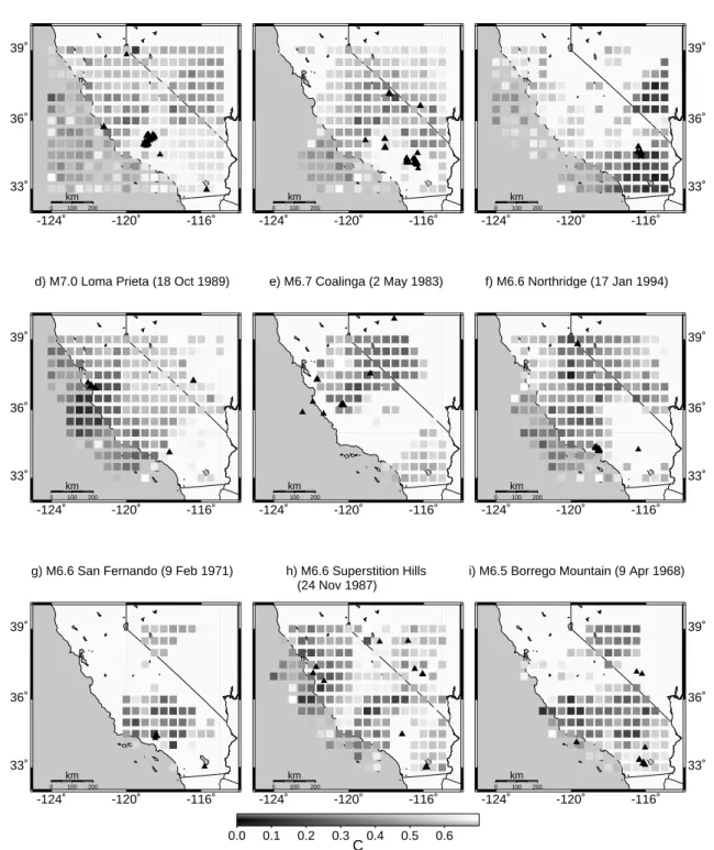
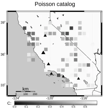
Results for the correlation length from Eq. (2) are shown in Fig. 2. The triangles are the earthquakes with M ≥ 5.0 oc-curring during one year after the strong shock with M ≥ 6.5 (largest triangle), i.e. the pattern Qi(x). The grey shaded boxes denote the GCL pattern Ci(x). Analogously, Fig. 3 is the same for a catalogue from the Poisson process model. Curvature parameters above 0.7 are not shown, since power laws and constant functions are no longer distinguishable.
The likelihood ratio test introduced in Sect. 2 is now ap-plied to compare the patterns Ci(x) and CiAPC(x) with the pattern Qi(x). The quantity Ni
s (0 ≤ Ns ≤ 100), which is the number of APCs that fit better to Qi(x) than the orig-inal data, is used as a measure for the predictive power of the GCL pattern in the original catalogue before a certain strong earthquake. Note that we do not introduce alarm con-ditions using threshold values. The results for Nsi are given in Table 1. The confidence level pconf in the last row is the probability that nine random numbers (corresponding to the nine strongest earthquakes) have a mean value smaller than or equal to hNsi =(1/9)PiNsi.
The spatial correlations of the GCL patterns with the fu-ture seismicity are clearly visible in some cases, e.g. the Hector Mine, the Loma Prieta, the Coalinga, and the San Fernando earthquakes. The most conspicuous anomaly can be observed prior to the Loma Prieta earthquake in Fig. 2d.
96 G. Z¨oller and S. Hainzl: Critical point dynamics
a) M7.5 Kern County (21 Jul 1952)
-124˚ -120˚ -116˚ 33˚ 36˚ 39˚ 0 100 200 km b) M7.3 Landers (28 Jun 1992) -124˚ -120˚ -116˚ 0 100 200 km
c) M7.1 Hector Mine (16 Oct 1999)
-124˚ -120˚ -116˚ 33˚ 36˚ 39˚ 0 100 200 km
d) M7.0 Loma Prieta (18 Oct 1989)
-124˚ -120˚ -116˚ 33˚ 36˚ 39˚ 0 100 200 km e) M6.7 Coalinga (2 May 1983) -124˚ -120˚ -116˚ 0 100 200 km f) M6.6 Northridge (17 Jan 1994) -124˚ -120˚ -116˚ 33˚ 36˚ 39˚ 0 100 200 km
g) M6.6 San Fernando (9 Feb 1971)
-124˚ -120˚ -116˚ 33˚ 36˚ 39˚ 0 100 200 km 0.0 0.1 0.2 0.3 0.4 0.5 0.6 C h) M6.6 Superstition Hills (24 Nov 1987) -124˚ -120˚ -116˚ 0 100 200 km
i) M6.5 Borrego Mountain (9 Apr 1968)
-124˚ -120˚ -116˚ 33˚ 36˚ 39˚ 0 100 200 km
Fig. 2. Curvature parameter C (grey shaded boxes) based on the GCL pattern. The filled triangles are the strong earthquakes (largest triangle)
and the earthquakes with M ≥ 5.0 until one year after these events.
This is probably due to the fact that there had been no other strong earthquake in the Loma Prieta region since 1910 and consequently, the GCL pattern of this event is not disturbed by the overlapping patterns from the other events. In con-trast, the result for the Kern County earthquake is close to a random response. A possible explanation is that the quality and the length of the data may not be sufficient prior to 1952.
As we have checked, the result for the Kern County event can be slightly improved with a magnitude cutoff of Mcut = 4.5 instead of Mcut = 4.0. The confidence level pconf = 89% for the nine strongest earthquakes is below the typical con-fidence levels for statistical hypothesis tests, e.g. p = 95%. However, if the Kern County earthquake is excluded from the analysis due to a lack of data quality, we obtain hNsi =32
0.0 0.1 0.2 0.3 0.4 0.5 0.6 C:
Poisson catalog
-124˚ -120˚ -116˚ 33˚ 36˚ 39˚ 0 100 200 kmFig. 3. Curvature parameter C (grey shaded boxes) with respect to
a strong earthquake (M = 7.0) for an adjusted Poisson catalogue (APC). The filled triangles are the earthquakes with M ≥ 5.0 until one year after these events.
and a resulting probability of pconf = 97%. In this case, the null hypothesis where the results can be reproduced using a realistic Poisson process model without spatiotemporal cor-relations is rejected with a reasonable high confidence level. We want to point out that all parameters in our analysis are fixed empirically or determined by the optimization tech-niques described in the previous section. This is a first or-der approach which may ignore important information in the data, leading to small significances. Therefore, it is important to determine parameters by physical conditions, e.g. scal-ing relations such as log R = c1+c2Mwith constants c1
and c2for the space window R (Bowman et al., 1998; Z¨oller
et al., 2001) and log T = c3+c4M with constants c3 and
c4 for the time window T (Hainzl et al., 2000), as well as
search magnitudes should be introduced in order to increase the significances. This would also be a step towards a pre-diction algorithm, where a spatiotemporal search for anoma-lies can be conducted. By introducing threshold values in terms of alarm conditions, an analysis by means of error di-agrams (Molchan, 1997) could then be carried out. These refinements and extensions are left for future studies.
4 Summary and conclusions
We have tested the hypothesis that spatial anomalies accord-ing to the critical point concept for earthquakes occur before strong earthquakes. Therefore, we have used the growing spatial correlation length as an indicator for critical point be-haviour. To reduce the number of free parameters, we have
fixed the magnitude cutoff and the critical exponent by val-ues known from the literature. The remaining parameters, namely, space and time windows have been determined sys-tematically by an optimization technique. From a likelihood ratio test in combination with a sophisticated Poisson process model, we have extracted a statistical confidence level.
By applying a search algorithm in space, we find a rough agreement of the predicted regions with future seismicity. Although false alarms and false negatives are present, the original data provide significantly better results than the Pois-son process model. The confidence level of 89% is enhanced by excluding the Kern County (1952) earthquake due to a lack of data quality. Further improvements in both the GCL model itself and the statistical test are possible. In particular, it is desirable to map directly probabilities instead of curva-ture values. This would allow one to compare the present analysis with similar approaches, especially with models based on accelerating energy/moment release.
In conclusion, we have shown that the critical point con-cept makes a contribution to the improvement of the seismic hazard assessment. Further studies and applications of the methods are promising to increase the significance of the re-sults.
Acknowledgements. This work was supported by the Deutsche
Forschungsgemeinschaft (SFB 555 and SCH280/13–1). The earth-quake data used in this study have been provided by the Northern California Earthquake Data Center (NCEDC) and include contribu-tions of the member networks of the Council of the National Seis-mic System (CNSS). To produce the figures, we used the GMT sys-tem (Wessel and Smith, 1991).
References
Bowman, D. D., Oullion, G., Sammis, C. G., Sornette, A., and Sor-nette, D.: An observational test of the critical earthquake con-cept, J. Geophys. Res., 103, 24 359–24 372, 1998.
Brehm, D. J. and Braile, L. W.: Intermediate-term earthquake pre-diction using precursory events in the New Madrid Seismic Zone, Bull. Seismol. Soc. Am., 88, 564–580, 1998.
Brehm, D. J. and Braile, L. W.: Intermediate-term earthquake pre-diction using the modified time-to-failure method in southern California, Bull. Seismol. Soc. Am., 89, 275–293, 1999. Bufe, C. G. and Varnes, D. J.: Predictive modeling of the seismic
cycle of the greater San Francisco Bay region, J. Geophys. Res., 98, 9871–9883, 1993.
Das, S. and Scholz, C. H.: Theory of time-dependent rupture in the Earth, J. Geophys. Res., 86, 6039–6051, 1981.
Gross, S. and Rundle, J.: A systematic test of time-to-failure analy-sis, Geophys. J. Int., 133, 57–64, 1998.
Gutenberg, B. and Richter, C. F.: Earthquake magnitude, intensity, energy and acceleration, Bull. Seismol. Soc. Am., 46, 105–145, 1956.
Hainzl, S. and Z¨oller, G.: The role of disorder and stress concen-tration in nonconservative fault systems, Physica A, 294, 67–84, 2001.
Hainzl, S., Z¨oller, G., and Kurths, J.: Similar power laws for foreshock and aftershock sequences in a spring-block model for earthquakes, J. Geophys. Res., 104, 7243–7253, 1999.
98 G. Z¨oller and S. Hainzl: Critical point dynamics
Hainzl, S., Z¨oller, G., Kurths, J., and Zschau, J.: Seismic quiescence as an indicator for large earthquakes in a system of self-organized criticality, Geophys. Res. Lett., 27, 597–600, 2000.
Jaum´e, S. C. and Sykes, L. R.: Evolving towards a critical point: A review of accelerating seismic moment/energy release prior to large and great earthquakes, Pageoph, 155, 279–306, 1999. Leckie, F. A. and Hayhurst, D. R.: Constitutive equations for creep
rupture, Acta Metall., 25, 1059–1070, 1977.
Molchan, G. M.: Earthquake prediction as a decision-making prob-lem, Pageoph, 149, 233–247, 1997.
Omori, F.: On the aftershocks of earthquakes, J. Coll. Sci. Imp.
Univ. Tokyo, 7, 111–200, 1894.
Reasenberg, P.: Second-order moment of central California seis-micity, J. Geophys. Res., 90, 5479–5495, 1985.
Wessel, P. and Smith, W. H. F.: Free software helps map and display data, Eos Trans., AGU, 72, 441, 445–446, 1991.
Z¨oller, G., Engbert, R., Hainzl, S., and Kurths, J.: Testing for un-stable periodic orbits to characterize spatiotemporal dynamics, Chaos, Solitons and Fractals, 9, 1429–1438, 1998.
Z¨oller, G., Hainzl, S., and Kurths, J.: Observation of growing corre-lation length as an indicator for critical point behaviour prior to large earthquakes, J. Geophys. Res., 106, 2167–2176, 2001.