Lire le début de la thèse

Lire

le début

de la thèse

Conclusions et Perspectives

Dans son document de synth`ese dat´e de 2014, l’Atelier de R´eflexion Prospective REAGIR d´efinit la g´eo-ing´enierie de l’environnement comme l’ensemble des techniques et pratiques mises en œuvre ou projet´ees dans une vis´ee corrective `a grande ´echelle d’ef-fets r´esultants de la pression anthropique sur l’environnement. Ces techniques doivent ˆetre distingu´ees des mesures classiques d’att´enuation (r´eduction des ´emissions de gaz `a effet de serre) ou d’adaptation (r´eduction de la vuln´erabilit´e des syst`emes naturels et humains aux effets des changements climatiques), mˆeme si elles peuvent `a certains ´egards les recouper. De par leur nature globale, elles revˆetent de nombreux enjeux (faisabilit´e technique, gouvernance, acceptabilit´e sociale) qui d´epassent largement le cadre de cette th`ese.

Deux grandes familles de techniques de g´eo-ing´enierie sont couramment distingu´ees. Les techniques d’extraction du dioxyde de carbone (CDR, Carbon Dioxide Removal) englobent toutes les m´ethodes ayant pour but la capture directe du CO2atmosph´erique

ou d’autres gaz `a effet de serre. Les techniques de gestion du rayonnement, le plus souvent solaire, (SRM, Solar Radiation Modification) regroupent toutes les m´ethodes ayant pour but d’affecter le climat par modification des flux radiatifs. Elles peuvent ˆetre d´eclin´ees en diff´erentes strat´egies consistant i) `a modifier l’alb´edo des surfaces terrestres, ii) `a modifier l’alb´edo des nuages (en pulv´erisant par exemple des sels marins dans la basse troposph`ere), iii) `a limiter le rayonnement solaire incident au sommet de la troposph`ere (en mettant en orbite des panneaux r´efl´echissant ou en injectant des a´erosols dans la stratosph`ere).

C’est `a cette derni`ere m´ethode de SRM que nous nous sommes int´eress´es, `a l’instar des premi`eres simulations de g´eo-ing´enierie (G1 et G4) mises en œuvre dans le cadre du projet international d’intercomparaison GeoMIP. Les Chapitres 3 et 4 ont port´e ex-clusivement sur l’injection de soufre dans la stratosph`ere (SRM-SAI, exp´erience G4), visant `a cr´eer des a´erosols d’acide sulfurique ayant comme propri´et´e de r´efl´echir le rayonnement solaire incident. L’injection pr´econis´ee se ferait dans la stratosph`ere tro-picale car le soufre inject´e sous forme gazeuse ou particulaire pourrait se disperser dans les deux h´emisph`eres via la circulation de Brewer-Dobson, influen¸cant ainsi le contenu en a´erosols stratosph´eriques `a l’´echelle globale et de mani`ere relativement homog`ene. Le mod`ele syst`eme Terre du CNRM, comme de nombreux autres mod`eles ayant par-ticip´e `a la premi`ere phase de GeoMIP, ne simule pas explicitement la chimie du soufre

et se contente de prescrire directement des charges en a´erosols stratosph´eriques. Les techniques de SRM-SAI s’inspirent du refroidissement de la surface de la Terre observ´e apr`es les grandes ´eruptions volcaniques qui sont associ´ees `a des injections de grandes quantit´es de soufre dans la stratosph`ere. Ce refroidissement est temporaire et ne dure que quelques ann´ees, le temps que les a´erosols d’acide sulfurique d’origine volcanique soient ´elimin´es de l’atmosph`ere. L’objectif de la SRM-SAI est d’obtenir un refroidissement “permanent” de la surface en injectant continuellement du soufre de mani`ere `a maintenir une couche d’a´erosols stratosph´eriques suffisante pour limiter l’effet de l’accroissement de l’effet de serre. L’´eruption volcanique du Mont Pinatubo en 1991 a inject´e 20 Mt de dioxyde de soufre dans la stratosph`ere et a g´en´er´e un refroidissement global d’un demi-degr´e environ pendant la premi`ere ann´ee. Cependant, il n’est pas acquis que l’injection continue de 20 Mt de dioxyde de soufre durant un an produise une couche d’a´erosols d’acide sulfurique comparable `a celle produite par l’´eruption volcanique du Mont Pinatubo en termes de distribution en taille d’a´erosols et donc en termes de for¸cage radiatif.

La question de l’efficacit´e de la SRM-SAI et de la quantit´e d’a´erosols `a injecter pour obtenir un refroidissement donn´e est donc une premi`ere question essentielle et a fait en partie l’objet du Chapitre 3. ´Etant donn´e la relative rusticit´e de la repr´esentation des a´erosols dans la g´en´eration CMIP5 des mod`eles utilis´es pour les exp´eriences G4 disponibles, les protocoles CMIP5 de GeoMIP ont fait preuve d’un certain laxisme quant au mode de repr´esentation des a´erosols dans ces exp´eriences (augmentation de l’AOD versus simulation de l’injection, diff´erences de profils latitudinaux et/ou verticaux de l’AOD/du SO2). Cela a conduit `a des r´esultats tr`es divergents en termes

d’att´enuation du rayonnement et de diminution de la temp´erature en moyenne globale, ce qui nous a pouss´e `a nous focaliser sur le refroidissement normalis´e par la r´eduction du rayonnement solaire incident en surface. Pour aller plus loin sur l’impact radiatif direct des a´erosols stratosph´eriques simul´es, nous avons mˆeme utilis´e le param`etre ”en ciel clair” qui permet de s’affranchir de la r´etroaction nuageuse. Ainsi, nous avons identifi´e une propri´et´e statistique entre le comportement des mod`eles dans l’exp´erience G4, et leur r´eponse aux principales ´eruptions du XX`eme_{si`ecle. Appuy´e par un jeu de donn´ees}

d’observations et de r´eanalyses aussi diversifi´e que possible, nous avons revu `a la baisse l’efficacit´e de la SRM-SAI par rapport `a la moyenne multi-mod`ele (r´eduction de 20%), et r´eduit l’incertitude associ´ee de 40%. N’oublions pas que ce travail visait `a contraindre l’incertitude en temp´erature pour un changement radiatif donn´e, sans se pr´eoccuper des processus pr´ealables reliant la strat´egie d’injection `a la d´estabilisation du bilan radiatif. Il est primordial de comprendre et d’´etudier l’ensemble des processus allant du choix des compos´es inject´es, en passant par leur taille, leur lieu d’injection, puis leur dispersion dans la haute atmosph`ere, leurs propri´et´es optiques, menant finalement au refroidissement de la plan`ete. Le r´ecent rapport sp´ecial du GIEC sur le sc´enario climatique 1.5°C en lien avec les accords de Paris stipule que la SRM pourrait limiter un ´eventuel overshoot en temp´erature au cours du XXI`eme _{si`ecle : l’importance de}

relier la strat´egie d’injection au refroidissement global effectif est donc primordiale quand il est question de ne pas d´epasser un seuil en temp´erature. L’am´elioration des connaissances passera ´egalement par l’´elaboration de protocoles plus sophistiqu´es, et plus en ad´equation avec les ´eventuelles techniques de mise en œuvre de la SAI.

d’emballement du r´echauffement global. Il a notamment ´et´e sugg´er´e que la SRM-SAI pourrait par ailleurs avoir des retomb´ees positives sur le cycle du carbone, en favorisant les puits naturels de carbone atmosph´erique que repr´esentent les oc´eans et les surfaces continentales. Ces puits naturels ont absorb´e pr`es de la moiti´e des ´emissions anthro-piques de CO2 sur la derni`ere d´ecennie, avec une contribution un peu plus forte pour

les surfaces continentales que pour l’oc´ean global. Le r´echauffement global et l’aridifi-cation ´eventuelle d’une partie des continents pourraient cependant r´eduire l’efficacit´e de ces puits naturels de carbone `a plus ou moins long terme. Le Chapitre 4 de cette th`ese a permis d’´evaluer l’impact de la SRM-SAI sur le bilan de carbone, d’une part `a moyen terme pendant la p´eriode de mise en œuvre de la SAI (2020-2070), mais aussi `a plus long terme en cas d’arrˆet de cette technique et en r´eponse `a un ´eventuel effet rebond sur la temp´erature globale. Les mod`eles s’accordent `a pr´edire que le climat induit par la SAI tend `a stimuler les puits naturels de carbone, principalement celui que constitue la biosph`ere continentale. La quantit´e additionnelle de carbone stock´e durant les 50 ann´ees de SAI serait de 40 GtC, ´equivalent `a 4 ann´ees d’´emissions an-thropiques au taux d’´emission actuel. N´eanmoins, plusieurs ´el´ements limitent l’impact a priori positif de la SAI sur les flux de carbone. En plus de l’incertitude sur l’ampli-tude de la r´eponse du cycle du carbone, notamment en lien avec l’incertil’ampli-tude sur la r´eponse du bilan radiatif et de la temp´erature d´ecrite dans le Chapitre 3, les mod`eles divergent sur les processus biog´eochimiques pilotant le signal. La compr´ehension des processus photosynth´etique et de respirations ainsi que leurs impl´ementations dans les mod`eles de climat n´ecessitent des ´etudes suppl´ementaires. Les am´eliorations qui ont ´et´e apport´ees au mod`ele du CNRM en vue du prochain exercice CMIP6 pourraient affiner les r´esultats obtenues dans cette ´etude (meilleur r´ealisme des processus de respi-rations, impact du rayonnement diffus sur la photosynth`ese...). Enfin, l’arrˆet prolong´e de la SAI provoquant un rebond en temp´erature dˆu `a l’effet de serre additionnel imput´e aux ´emissions de CO2 anthropique impliquerait une r´eversibilit´e du cycle du carbone,

le carbone accumul´e durant la p´eriode de SAI serait alors rapidement relˆach´e dans l’atmosph`ere.

Bien que l’acceptabilit´e sociale et la gouvernance de la g´eo-ing´enierie ne soient pas le sujet de cette th`ese, il semble pour le moment acquis que toute d´ecision de mise en œuvre devrait se faire de mani`ere concert´ee (dans le cadre des Nations Unies) et avec l’accord de tous les pays. Sur le plan scientifique, cela signifie que la possibi-lit´e de compenser le r´echauffement global anthropique via cette technique ne garantit nullement son approbation tant que ses potentiels effets collat´eraux ne sont pas do-cument´es, y compris `a l’´echelle r´egionale. `A titre d’illustration, et ind´ependamment des effets attendus sur l’acidit´e des oc´eans ou sur l’ozone stratosph´erique, le Chapitre 5 s’est int´eress´e `a l’impact de la SRM sur le climat hivernal de l’Europe. Diverses sources d’incertitudes sur cette r´eponse ont ´et´e explor´ees : le choix du mod`ele uti-lis´e (comparaison des mod`eles CNRM-ESM1 et CNRM-ESM2.1 dans les simulations G1), mais aussi le choix du protocole mis en œuvre (comparaison des exp´eriences G1 et G4) avec le mod`ele CNRM-ESM1. Ces deux ´etudes parall`eles montrent la sensi-bilit´e de la r´eponse climatique et l’incertitude existante entre les r´eponses de deux mod`eles aux paradigmes pourtant communs, et entre deux simulations pourtant pi-lot´ees par les mˆemes scientifiques. Les efforts de mod´elisation du syst`eme climatique

sont donc essentiels afin de r´eduire les incertitudes li´ees aux simplifications de certains processus, hypoth`eses n´ecessaires `a la mod´elisation climatique mais qui ne doivent pas alt´erer les r´esultats scientifiques. Dans le cas du mod`ele du CNRM, l’am´elioration de la repr´esentation verticale de l’atmosph`ere notamment l’augmentation de l’altitude du toit du mod`ele permet de mieux repr´esenter la dynamique stratosph´erique, n´ecessaire quand il s’agit d’´etudier des simulations de type SAI.

Pour r´esumer cette th`ese, on peut donc conclure que les techniques de SRM-SAI ne sont pas aussi s´eduisantes que ce qu’en disent leurs avocats ou promoteurs. Les quantit´es de soufre `a injecter dans la stratosph`ere, et les coˆuts aff´erents, pour contre-carrer l’effet de l’accroissement des gaz `a effet de serre sur la temp´erature du globe pourraient ˆetre plus ´elev´es que pr´evu. Les retomb´ees positives sur le cycle du carbone restent tr`es hypoth´etiques dans l’´etat actuel de la mod´elisation du syst`eme Terre et se-ront largement annihil´ees en cas d’arrˆet de l’injection de soufre (ou d’autres pr´ecurseurs d’a´erosols) dans la stratosph`ere. Enfin et surtout, si la r´eduction du rayonnement so-laire incident permet effectivement de compenser l’effet des ´emissions anthropiques de gaz `a effet de serre sur la temp´erature de surface en moyenne annuelle et globale, cette compensation reste tr`es imparfaite sur la r´epartition verticale et latitudinale des temp´eratures, ce qui peut engendrer des r´epercussions n´egatives sur la circulation atmosph´eriques et les pr´ecipitations `a l’´echelle r´egionale.

D’autres effets collat´eraux potentiellement importants ont ´et´e mis en ´evidence par d’autres ´etudes, tels qu’une diminution de la couche d’ozone stratosph´erique, notam-ment en Antarctique, tant que subsistera une teneur ´elev´ee de compos´es halog´en´es dans la stratosph`ere, ce qui sera le cas pendant encore de nombreuses d´ecennies. La repr´esentation fine de la stratosph`ere dans CNRM-ESM2.1 (r´esolution verticale, simu-lation r´ealiste de la QBO, des vortex polaires et des r´echauffements stratosph´eriques soudains dans les deux h´emisph`eres, ozone interactif via le mod`ele de chimie stra-tosph´erique REPROBUS) est un atout important pour explorer cette question dans la continuit´e de cette th`ese. Une autre perspective `a court terme est d’utiliser les prochaines simulations GeoMIP r´ealis´ees dans le cadre de CMIP6 pour confirmer ou non la sensibilit´e de la r´eponse de la dynamique stratosph´erique au choix du mod`ele et/ou du protocole utilis´e, et quantifier les incertitudes associ´ees en termes de climat sur l’Atlantique Nord et sur l’Europe. Dans cette optique, l’utilisation de grands en-sembles pourrait s’av´erer pr´ecieuse pour d´etecter significativement le signal r´egional de la SRM, notamment sur les pr´ecipitations.

`A un peu plus long terme, la strat´egie mise en œuvre dans le Chapitre 3 pour contraindre la r´eponse thermique globale `a la r´eduction du rayonnement solaire in-cident pourrait ˆetre appliqu´ee `a l’´echelle plus r´egionale et/ou `a d’autres variables. N´eanmoins, l’utilisation des ´eruptions volcaniques comme analogue de la SRM-SAI r´eside principalement dans la m´ethode actuelle de mod´elisation de la SAI dans les mod`eles de climat. L’´elaboration de protocoles plus sophistiqu´es, en adaptant par exemple le lieu ou la saisonnalit´e de l’injection, ou encore les propri´et´es des a´erosols ou de leurs pr´ecurseurs, pourrait r´eduire l’analogie qui peut ˆetre faite aujourd’hui entre les ´eruptions volcaniques et la SRM-SAI dans les mod`eles de climat.

Au sein de la communaut´e scientifique, les diff´erentes techniques de SRM ont sou-vent ´et´e mises dans le mˆeme panier, pensant que les impacts climatiques seraient semblables. La comparaison de protocoles de nature diff´erente a montr´e que les

im-g´en´eraliser les conclusions `a l’ensemble des techniques de SRM. L’exercice GeoMIP pour CMIP6 pr´evoit par exemple d’´etudier la technique d’amincissement des cirrus par acc´el´eration de la s´edimentation de leurs cristaux de glace.

Enfin, outre les incertitudes scientifiques sur les multiples effets climatiques de la SRM-SAI, ce projet de g´eo-ing´enierie pose des probl`emes majeurs de gouvernance mondiale. L’´echec relatif de cette derni`ere dans la lutte contre le r´echauffement clima-tique laisse pr´esager des difficult´es analogues `a propos de la gouvernance de la SRM. Des travaux interdisciplinaires, mˆelant sciences “dures” et sciences humaines (sociales, politiques et de l’´ethique) doivent donc ˆetre men´es sur cette th´ematique, sans se faire au d´etriment des travaux en cours visant `a identifier et si possible lever les verrous techniques, sociaux et politiques d’une r´eduction substantielle des ´emissions de gaz `a effet de serre. Cette r´eduction drastique des ´emissions reste la principale solution pour limiter le r´echauffement global et ses impacts. Pour la majorit´e des scientifiques, la g´eo-ing´enierie reste un plan B tr`es imparfait et tr`es hypoth´etique, mais sur lequel on ne peut faire l’impasse tant que p`ese la menace de changements climatiques abrupts et/ou irr´eversibles.

1.1 S´erie temporelle des ´emissions anthropiques de carbone . . . 3

1.2 Mappemonde des exp´eriences de g´eo-ing´enierie . . . 4

1.3 Figure du rapport sp´ecial du GIEC (SR15) . . . 5

2.1 Syst`eme climatique . . . 11

2.2 Profil vertical de la temp´erature atmosph´erique . . . 12

2.3 Param`etres orbitaux de la Terre . . . 16

2.4 For¸cages climatiques au cours du dernier mill´enaire . . . 17

2.5 Position de la g´eo-ing´enierie, entre mitigation et adaptation . . . 21

2.6 Principaux concepts de la g´eo-ing´enierie (ARP REAGIR) . . . 22

2.7 ´Evolution de la repr´esentation du syst`eme climatique dans les mod`eles . 24 2.8 Impact de la r´esolution horizontale sur le relief . . . 25

2.9 ´Evaluation de CNRM-ESM1 et CNRM-ESM2-1 : TAS . . . 28

2.10 ´Evaluation de CNRM-ESM1 et CNRM-ESM2-1 : PR . . . 29

2.11 ´Evaluation de CNRM-ESM1 et CNRM-ESM2-1 : GPP . . . 30

3.1 Sch´ema de la simulation G4 . . . 37

3.2 R´eponse globale `a la SRM-SAI : (a) SWcs (b) T (c) PR . . . 39

3.3 R´eponse r´egionale `a la SRM-SAI : SWcs . . . 40

3.4 R´eponse r´egionale : T . . . 41

3.5 R´eponse r´egionale `a la SRM-SAI : PR . . . 41

3.6 For¸cages volcaniques : AOD sur la p´eriode historique . . . 44

3.7 R´eponse globale aux ´eruptions volcaniques : SWcs . . . 48

3.8 R´eponse globale aux ´eruptions volcaniques : T . . . 50

3.10 R´eponse r´egionale aux ´eruptions volcaniques : T . . . 52

3.11 R´eponse r´egionale aux ´eruptions volcaniques : PR . . . 53

3.12 Sch´ema de la m´ethode de contrainte ´emergente . . . 65

4.1 S´erie temporelle des sources et puits de carbone (GCP) . . . 70

4.2 R´eponse de la GPP dans CNRM-ESM1 . . . 101

4.3 Coefficients α des mod`eles lin´eaires . . . 104

4.4 Flux bruts (GPP, RA, RH) pour les deux mod`eles japonais MIROC . . 106

5.1 Sch´ema de la simulation G1 . . . 111

5.2 Comparaison CNRM-ESM1 / CNRM-ESM2-1 : coupe zonale DJF TA . 115 5.3 Comparaison CNRM-ESM1 / CNRM-ESM2-1 : coupe zonale DJF UA 117 5.4 Comparaison CNRM-ESM1 / CNRM-ESM2-1 : zoom Europe DJF TAS 119 5.5 Comparaison CNRM-ESM1 / CNRM-ESM2-1 : zoom Europe DJF U850120 5.6 Comparaison CNRM-ESM1 / CNRM-ESM2-1 : zoom Europe DJF PR 121 5.7 Comparaison CNRM-ESM1 / CNRM-ESM2-1 : zoom Europe DJF P−E122 5.8 Comparaison G1 / G4 : coupes zonales DJF TA et UA . . . 124

5.9 Comparaison G1 / G4 : zoom Europe DJF TAS, U850 et PR . . . 126

C.1 PAR interactif : GPP et LAI . . . 168

C.2 PAR interactif : TAS et PR . . . 169

D.1 Comparaison CNRM-ESM1 / CNRM-ESM2-1 : carte globale DJF TAS 172 D.2 Comparaison CNRM-ESM1 / CNRM-ESM2-1 : carte globale JJA TAS 173 D.3 Comparaison CNRM-ESM1 / CNRM-ESM2-1 : carte globale DJF U850 174 D.4 Comparaison CNRM-ESM1 / CNRM-ESM2-1 : carte globale JJA U850 175 D.5 Comparaison CNRM-ESM1 / CNRM-ESM2-1 : carte globale DJF PR . 176 D.6 Comparaison CNRM-ESM1 / CNRM-ESM2-1 : carte globale JJA PR . 177

2.1 Comparaison des composantes de CNRM-ESM1 et de CNRM-ESM2-1 . 26

2.2 R´esolutions des mod`eles CMIP5 . . . 31

3.1 Mod`eles GeoMIP : param´etrage SRM-SAI . . . 46

3.2 Mod`eles GeoMIP : param´etrage des ´eruptions volcaniques . . . 47

4.1 Bilan des flux de carbone cumul´es sur la p´eriode de SRM-SAI . . . 102

Midlatitude Summer Drying : An

Underestimated Threat in CMIP5

Models ?, Geophysical Research

Letters,

Douville and Plazzotta

Midlatitude Summer Drying: An Underestimated

Threat in CMIP5 Models?

H. Douville1 _{and M. Plazzotta}1

1_{Météo-France/CNRM, Toulouse, France}

Abstract Early assessments of the hydrological impacts of global warming suggested both an intensification of the global water cycle and an expansion of dry areas. Yet these alarming conclusions were challenged by a number of latter studies emphasizing the lack of evidence in observations and historical simulations, as well as the large uncertainties in climate projections from the fifth phase of the Coupled Model Intercomparison Project (CMIP5). Here several aridity indices and a two-tier attribution strategy are used to demonstrate that a summer midlatitude drying has recently emerged over the northern continents, which is mainly attributable to anthropogenic climate change. This emerging signal is shown to be the harbinger of a long-term drying in the CMIP5 projections. Linear trends in the observed aridity indices can therefore be used as observational constraints and suggest that the projected midlatitude summer drying was underestimated by most CMIP5 models. Mitigating global warming therefore remains a priority to avoid dangerous impacts on global water and food security.

Plain Language Summary What will be the consequence of global warming on regional soil moisture at the end of the 21st century? The response found in the fifth Assessment Report (AR5) of Intergovernmental Panel on Climate Change is blurred by many uncertainties, even when the focus is on a single business-as-usual scenario for the projected concentrations of greenhouse gases. Such a confusion is dominated by climate model uncertainties on the long term but might be also due to internal climate variability on the near term. Here we use a detection-attribution methodology to demonstrate that recent trends in soil moisture and in near-surface relative humidity averaged over the boreal midlatitude continents in summer have been mainly driven by human activities. Then we show that there is a fairly strong relationship between the near-term versus long-term aridity response among a set of 20 climate models, thereby supporting the limited influence of internal climate variability on near-term variability. Finally, we use this emergent relationship to constrain the long-term model response with the recent trends estimated from the observations and find that the projected long-term drying was probably underestimated by most global climate models explored in the AR5.

1. Introduction

Water scarcity is a major threat for food security and economic prosperity in many countries, which is not expected to decrease given the growing global population and related pressure on available water resources. Moreover, the global water cycle might be seriously affected by the projected climate change due to anthro-pogenic emissions of greenhouse gases (GHGs). The threat of an increased risk of drought, including in the summer midlatitudes, was highlighted by both empirical (e.g., Dai et al., 2004) and numerical studies (e.g., Douville et al., 2002; Frierson & Scheff, 2012; Scheff & Frierson, 2015). Off-line hydrological simulations suggest that a global warming of 2°C above present will increase the population living under extreme water scarcity by another 40% compared with the effect of population growth alone (e.g., Schewe et al., 2014). Nevertheless, such hydrological impacts are highly model dependent, with both global climate models (GCMs) and off-line land surface models (LSMs) contributing to the spread. Internal climate variability is also a major source of uncertainty, even if the model formulation generally dominates the spread by the end of the 21st century (Orlowsky and Seneviratne, 2013).

In contrast to the mainstream thinking, a number of studies cast serious doubts on the reality of the ongoing and/or projected global drying. First, empirical aridity indices must be interpreted cautiously since they rely on a simplified calculation of potential evaporation that may respond incorrectly to the land surface warming observed in recent decades (Joetzjer et al., 2013; Sheffield et al., 2012). Moreover, the general climate change paradigms that “dry regions are getting drier and wet regions are getting wetter” and that “warmer is more

Geophysical Research Letters

10.1002/2017GL075353

Key Points:

•Independent data sets are used to demonstrate the reality and anthropogenic origin of a recent multidecadal drying of the summer midlatitudes

•In CMIP5 models the summer drying projected at the end of the 21st century shows a significant relationship with the recent drying •This emergent relationship is used to

constrain the model response and suggests that most CMIP5 models underestimate the projected drying

Supporting Information: •Supporting Information S1 Correspondence to: H. Douville, herve.douville@meteo.fr Citation:

Douville, H., & Plazzotta, M. (2017). Midlatitude summer drying: An underestimated threat in CMIP5 models? Geophysical Research Letters, 44. https://doi.org/10.1002/ 2017GL075353

Received 17 AUG 2017 Accepted 28 SEP 2017

Accepted article online 4 OCT 2017

©2017. American Geophysical Union. All Rights Reserved.

arid” have been recently challenged (Greve et al., 2014, Roderick et al., 2015). When aridity changes are assessed as the lack of precipitation, the lack of runoff, or using a carbon budget approach, most global model outputs suggest that “warmer is less arid” (Roderick et al., 2015). In addition, rising atmospheric CO2is likely to decrease the plant

water use, a physiological process which is overlooked in many climate models and/or impact studies and which can reduce future drought stress (e.g., Best et al., 2007; Swan et al., 2016). Finally, Berg et al. (2016) found a robust vertical gradient of soil moisture anomalies in the fifth phase of the Coupled Model Intercomparison Project (CMIP5) models, with more negative changes projected near the surface, thereby suggesting that the surface drying predicted by empirical and/or off-line metrics may tend to exaggerate changes in total soil moisture availability.

The present study has a twofold objective: (i) attributing the recent variability and (ii) constraining the long-term evolution of total soil moisture and related variables over the northern midlatitude continent in summer (June to September, hereafter JJAS). The first objective is achieved by analyzing ensembles of global atmo-spheric simulations driven by the human-forced versus total variations of observed sea surface temperature (SST) and sea ice concentration (SIC). The second objective is achieved by using the diagnosed human-forced aridity trends as an emergent constraint for the aridity projections derived from a subset of 20 CMIP5 models. Given the lack of direct total soil moisture observations at the global scale, an off-line land surface reanalysis will be used as well as other (indirect) land surface aridity indices.

Section 2 describes the experiment design and the observed data sets. Results are shown in section 3. A recent land surface drying is found in multiple data sets, which is dominated by anthropogenic climate change. The implications of this attribution for aridity projections are also discussed in section 3 and suggests that this emerging signal is the harbinger of a much stronger drying, which was underestimated by most CMIP5 models. The main conclusions are drawn in section 4.

2. Experiment Design and Data Sets

With the increasing confidence that recent global warming is very likely due to human activities, detection and attribution (hereafter) D&A studies have recently moved from temperature to other climate variables equally relevant for impact studies. As far as the global water cycle is concerned, formal D&A studies have revealed a human influence on the zonal mean distribution of precipitation (e.g., Zhang et al., 2007) and sur-face evapotranspiration (e.g., Douville et al., 2012). Yet the net effect of such changes on the land sursur-face water budget is difficult to assess. D&A of observed changes in continental waters remains a difficult chal-lenge given the limited instrumental record and/or the direct human influence on rivers and reservoirs. To the author’s knowledge, the recent study by Mueller and Zhang (2016) is the only one that has been so far successful at attributing changes in soil moisture. The focus was on the northern continents and on the hot-test season. The analysis was limited to the 1951–2005 period and based on the comparison between soil moisture outputs from CMIP5 models versus LSMs.

Here the focus is also on the northern midlatitude continents and on the boreal summer season, but the study uses one more decade of data and a two-tier D&A strategy. First, a formal D&A algorithm is applied to isolate the SST and SIC variations driven by anthropogenic and/or natural radiative forcings (cf. supporting information (SI)). Then, ensembles of atmospheric-only global climate simulations are performed to attribute recent changes in soil moisture and related land surface variables. So doing, the CMIP5 models are only used to assess the externally forced variations in the SST observations. By prescribing the observed SST variability, our strategy enables a more straightforward comparison with the observations (e.g., Dai, 2013).

The experiment design is summarized in Table 1. Two ensembles of 1920–2014 global atmospheric simula-tions have been achieved. ALL is a nine-member ensemble of extended AMIP (Atmospheric Model Intercomparison Project) simulations driven by observed SST/SIC and radiative forcings. ANT is a five-member ensemble driven by the human-forced SST/SIC variability and the anthropogenic radiative forcings (no volca-nic eruption and no variation in solar activity). Note that two additional nine-member ensembles have been

Table 1

Summary of the Ensemble AGCM Experiments

Expt SST Radiative forcings Size

ALL Observed AMIP NAT + ANT 9

EXT Externally-Forced AMIP NAT + ANT 9

INT Internal AMIP Fixed 9

ANT Human-Forced AMIP ANT Only 5

Note. For the INT ensemble, “fixed” means the 1920–1960 monthly (SST and aerosols) or annual (other radiative forcings) mean climatology. Here the study is based on the ALL and ANT ensembles and the influence of the natural climate variability is estimated as the ALL minus ANT difference.

achieved to isolate the role of the internal versus externally forced climate variability (cf. Table 1). No ensem-ble is availaensem-ble to diagnose the influence of natural climate variability (i.e., internal variability + natural for-cings) so that this influence will be here estimated as the difference between the ALL and ANT ensembles. All experiments are based on version 6.2 of the ARPEGE-Climat AGCM, which is an update of v5.2 as described in Voldoire et al. (2013). The main differences between v5.2 and v6.2 include a modification of the vertical diffusion scheme and a new shallow and deep convection scheme. The land surface model has been also improved in many respects, including the introduction of a direct (biophysical) CO2effect on stomatal closure

(Joetzjer et al., 2015) and the representation of floodplains and groundwaters fully coupled to the soil hydrol-ogy. The groundwater scheme needs to be integrated for many decades to reach an equilibrium under pre-industrial climate conditions. Such a strategy was not here feasible given the limited computing resources and the decision to start the simulations in 1920. The different members of our experiments were initialized at 5 year intervals from a first extended AMIP integration after a minimum spin-up of 30 years. This is suffi-cient for most land surface variables to reach equilibrium. A residual drift of deep soil moisture is, however, discernible, which does not represent a major issue since the role of natural climate variability is assessed as the difference between the ALL and ANT ensembles (sharing the same drift).

As far as the CMIP5 models are concerned, all results are based on a single realization of the historical (1850– 2005) and corresponding RCP8.5 (2006–2100) simulations. Only a subset of 20 models (cf. Table S1 in SI) has been used to avoid or at least mitigate the issue of model interdependency when building emergent con-straints on model projections (Knutti et al., 2017). The main selection criterion was avoiding the use of several models based on the same atmospheric component. A second criterion was the availability of monthly mean model outputs not only for total soil moisture but also for the following variables: near-surface daily mean, daily minimum, and daily maximum temperatures (the latter two being used to assess the diurnal tempera-ture range, hereafter DTR); near-surface relative humidity (hereafter RH); and surface evaporative fraction (hereafter EF) estimated as the ratio between latent heat and total (latent + sensible) turbulent fluxes at the land-atmosphere interface.

The observational counterpart is based on the following data sets: the 1979–2010 European Centre for Medium-Range Weather Forecasts Re-Analysis Interim (ERAI)-Land off-line land surface reanalysis (Balsamo et al., 2015) for soil moisture, the 1979–2016 ERAI atmospheric reanalysis assimilating SYNOP observations (Dee et al., 2011) for RH and the global mean surface temperature (GMST), the 1901–2014 CRU_TS3.23 clima-tology (https://crudata.uea.ac.uk/cru/data/hrg/) for near-surface temperature, and the 1982–2011 Model Tree Ensemble (MTE) upscaling of in situ FLUXNET measurements (Jung et al., 2010) for EF. In addition to CRU_TS3.23, Hadex2 (http://www.metoffice.gov.uk/hadobs/hadex2/) was also used as an alternative gridded DTR data set and led to similar results.

Note that ERAI-Land is a land surface model simulation driven by observed meteorological forcings. The water budget is thereby perfectly closed, making ERAI-Land a more suitable soil moisture data set for climate applications than ERAI. Yet there is no soil moisture data assimilation so that it is important to use multiple aridity indices in the present study. Modern-Era Retrospective Analysis for Research and Applications (MERRA)-Land was not used as an alternative soil moisture reconstruction, since it shows less consistent trends than ERAI-Land when compared with satellite surface soil moisture over recent decades (Albergel et al., 2013). Additional data sets could have been explored, such as surface soil moisture, vegetation indices, or precipitation, but they would have been unavailable for most CMIP5 models and/or less connected to total soil moisture. Maps of correlations of JJAS anomalies indeed suggest that RH (Figure S1) and DTR (Figure S2) are strongly linked to total soil moisture at interannual timescales in both observations and the CNRM AGCM. Moreover, the simulated correlations are quite realistic in the northern midlatitudes, suggesting that these variables can be here considered as consistent surrogates for soil moisture.

In contrast, the correlation with EF (Figure S3) is stronger than inferred from reconstructions and does not show a clear transition between soil moisture versus energy-limited evapotranspiration around 55°N, as sug-gested by the ERAI-Land and MTE data sets. While this discrepancy might be the evidence of a too strong land-atmosphere coupling (e.g., Levine et al., 2016; Vilesa et al., 2017), it might be also due to inconsistencies between the reconstructed soil moisture and EF, the latter being based on an empirical upscaling technique and a very limited number of in situ observations. As a result, and owing to the limited length of this data set, we will not use the MTE reconstruction to constrain the CMIP5 projections in the continuation of the study.

Note finally that the ERAI-Land reanalysis uses a four-layer land surface model with uniform thicknesses, while soil depth is not uniform in most climate models and is highly model dependent in the CMIP5 archive. It is therefore necessary to standardize the soil moisture values for comparing the various data sets. This standar-dization (i.e., substracting the climatological mean and dividing by the climatological standard deviation) was here done after averaging the total soil moisture over the northern midlatitude domain (hereafter referred to as the SSM index). This choice avoids giving too strong an emphasis on small absolute soil moisture variations in arid areas and is more relevant to discussing the evolution of the regional land surface water budget.

3. Results

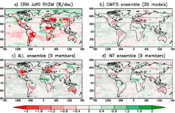
Figure 1 compares global maps of 1979–2014 linear trends in JJAS RH between ERAI and three ensembles of global atmospheric simulations: CMIP5, the ALL ensemble driven by observed SST and radiative forcings, and the INT ensemble driven by the internal variability of the observed SST and fixed radiative forcings (1920– 1960 climatology). In line with the results of Simmons et al. (2010) and with other data sets, ERAI shows large drying trends in many areas, including over most boreal midlatitude continents. This pattern is strongly underestimated by CMIP5 models although they also show consistent drying trends over North America and Europe. The ALL ensemble is globally more realistic even if the pattern shows some differences with ERAI. The INT ensemble hardly shows any trend in the midlatitudes, thereby suggesting that the drying simu-lated in the ALL ensemble is dominated by the external radiative forcings.

The hypothesis of a recent summer drying hiatus in most CMIP5 models is further supported by Figure S4 which mainly shows time series of JJAS land surface anomalies averaged over the boreal summer midlatitude continents. Note that this underestimated drying has not much to do with the recent global warming hiatus which shows a distinct spatial and seasonal signature (Trenberth et al., 2014). Figure S4 also highlights the large spread found in the CMIP5 projections, especially for the SSM index and the related land surface vari-ables. Even the sign of the response remains uncertain for DTR, EF, and SSM at the end of the 21st century. Such a dispersion raises the question of whether the recent model behavior is informative about their

Figure 1. Global distribution of 1979–2014 linear trends in JJAS surface air relative humidity (% per decade) in (a) the ERA-Interim Reanalysis, (b) a subset of 20 CMIP5 models, (c) the ALL ensemble driven by observed SST and radiative forcings, and (d) the INT ensemble driven by the internal variability of the observed SST and fixed (1920–1960 average) radiative forcings. Hatching denotes consistent trends among the different members of the ensembles using a t test at a 5% level.

long-term response and whether it can be assessed on the basis of a single simulation given the possible influence of internal climate variability.

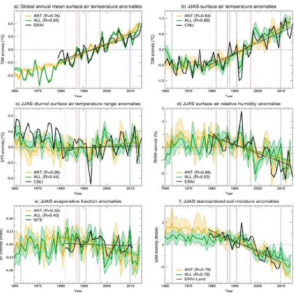
Before exploring this, Figure 2 compares the 1979–2014 linear trends between the ANT and ALL ensembles conducted with the CNRM AGCM to discuss the anthropogenic versus natural origin of the recent multideca-dal variability. The influence of the natural climate variability can be estimated as the difference between the ALL and ANT ensembles. The underlying assumption is that the atmospheric responses to individual radiative and/or SST forcings are additive. While such a hypothesis cannot be verified on the basis of our experiment design (cf. Table 1), the additivity of the JJAS midlatitude anomalies is verified in the case of the INT and EXT additional ensembles (not shown). The only noticeable exception is the total soil moisture response, in line with the residual drift discussed in section 2. Given our initialization strategy, this drift is however common

Figure 2. (a) Simulated versus ERAI time series of global annual mean surface air temperature anomalies (°C) from 1960 to 2015. Other panels show simulated time series of JJAS mean anomalies averaged over the northern midlatitude continents [35–55°N] for (b) surface air temperature (°C) versus CRU, (c) diurnal temperature range (°C) versus CRU, (d) surface air relative humidity (%) versus ERAI, (e) evaporative fraction versus MTE, and (f) standardized soil moisture anomalies versus ERAI-Land. For each ensemble (ALL in green and ANT in orange), the thick line denotes the ensemble mean, while the shaded area denotes the 95% confidence interval for the ensemble mean. Linear fits are estimated over the 1979–2014 period (except for shorter observational records). Vertical dashed lines denote JJAS seasons with major anomalies of global mean volcanic aerosol optical depth (in black) or Niño3–Niño4 SST (warm events in red and cold events in blue). R is the temporal correlation of the ensemble mean anomalies with the observed anomalies.

to all ensembles and is therefore suppressed when estimating the natural variability as the difference between ALL and ANT.

Starting with the annual mean GMST response as an illustration, the global warming trend simulated in the ANT ensemble is slightly stronger than in the ALL ensemble (Figure 2a), thereby suggesting a recent global cooling due to natural climate variability. In line with Douville et al. (2015), this relative cooling is primarily due to internal climate variability (not shown) and is not found over the boreal midlatitude continents in summer (Figure 2b). More interestingly, the robust drying trend simulated in the ALL ensemble is mainly attributable to the anthropogenic forcings (Figure 2c–2f). While the negative trend in total soil moisture (Figure 2f) is robust in both ALL and ANT, the former experiment is less consistent with ERAI-Land thereby suggesting that the CNRM AGCM slightly underestimates the “observed” midlatitude drying. Looking at the other compo-nents of the water budget (Figure S7), it seems that this feature is not due to an underestimation of the pre-cipitation decrease but rather to the evapotranspiration trend (although the MTE reference data set does not cover the whole 1979–2014 period and the linear trends are not significant over such a short period). The robust summer midlatitude drying simulated in ALL and ANT is also found in RH (Figure 2d) and is quite consistent with ERAI after 1979. It is also consistent with a recent increase in the simulated DTR, which is, how-ever, not found in the CRU data set. Yet a wider 1960–2014 perspective supports the trend reversal simulated at the end of the twentieth century in both ALL and ANT. This multidecadal variability is compatible with a dominant time-varying radiative effect of anthropogenic aerosols (Boé, 2016; Zhou et al., 2010). Such a hypothesis is supported by the sliding temporal correlations shown in the supporting information. While both RH and DTR are robust proxies of the SSM index (Figure S5), they are also sensitive to the variability of downward surface solar radiation (Figure S6). This radiative signature seems quite realistic in the CNRM AGCM, at least for the soil moisture and RH indices which can therefore be used to constrain the CMIP5 projections.

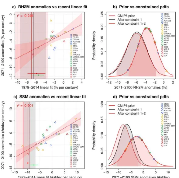
Figure 3 shows scatterplots of the long-term RH and SSM responses versus the recent linear trends estimated over the 1979–2014 period. As indicated by the squared correlations in Figures 3a and 3c, such trends explain 24 to 60% of the intermodel spread at the end of the 21st century. The idea that climate change is emerging in the instrumental record and can be used to constrain the long-term projections is not new (e.g., Knutti et al., 2017) but can be misleading if the observed trends are not dominated by anthropogenic forcings. Note that our CMIP5 ensemble (only one realization for each model) here samples both uncertainties in the model formulation and in the initial conditions. Yet internal climate variability can be considered as a ran-dom effect in these coupled simulations and has therefore a limited impact on the regression slope. More critical is the potential role of natural variability in the observed trends if one plans to use them as observational constraints. In both Figures 3a and 3c, the observed trends and their likely range (95% confi-dence interval) are shown as black lines and gray shadings, respectively. Also shown are the corresponding trends and confidence intervals in the ALL (green) and EXT (red) experiments. Not surprisingly, given the con-trasted fraction of the intermodel spread explained by the linear regressions, the confidence intervals are tighter and the difference between ALL and ANT is smaller for the SSM compared to RH index. Arguing that the human-induced linear trends represent a better constraint on the long-term response of the CMIP5 mod-els than the observed trends, the difference between ALL and ANT can be used to translate the observed trends on the x axis as represented by the maroon lines compared to the black lines. The confidence intervals are then also increased to account for the uncertainties in the ALL minus ANT differences.

Figures 3b and 3d illustrate the distribution of the CMIP5 model uncertainties and their potential reduction through the use of the emergent constraints shown in Figures 3a and 3c, respectively. The prior distribution (in red) is assumed to be Gaussian and is only estimated from the discrete realizations of the CMIP5 models. Using the observed 1979–2014 linear trends to constrain the projections through a simple calculation of con-ditional probabilities leads to a steeper distribution (in black) with a tighter 95% confidence interval (shading) and a drier ensemble mean response for both RH and SSM. This shift and narrowing is more important for soil moisture than for RH raising some questions about the consistency between both indices. Yet there is a qua-litative agreement between the two diagnostics whereby the summer drying of the northern midlatitude continents was underestimated by most CMIP5 models. Taking into account the additional constraint about the limited contribution of natural climate variability to the observed trends (cf. maroon pdfs) does not change this conclusion which is even slightly reinforced in the case of total soil moisture.

4. Summary

Several surface aridity indices have been explored in both CMIP5 models and global observations or reconstructions to assess trends over recent decades and their possible use as emergent constraints on the long-term projections. Focusing on the boreal summer midlatitude continents, the results suggest that such a strategy could be particularly efficient to constrain the late 21st century response of total soil moisture in RCP8.5 scenarios, provided the availability of reliable observations over three to four decades. In the lack of direct observations, the ERA-Interim land surface reanalysis suggests a strong underestimation of the recent and future soil drying in the CMIP5 models.

This result should be considered with caution given the nature of the ERAI-Land reanalysis (i.e., an off-line land surface simulation without data assimilation). Nevertheless, it is supported by a similar analysis based

Figure 3. (a) Scatterplot of 2071–2100 anomalies (%) versus 1979–2014 linear trends (% per century) of JJAS near-surface air relative humidity averaged over the northern midlatitude continents among a subset of 20 CMIP5 models and related linear regression (red line, 95% confidence interval in shading). (b) Prior (no observational constraints) and constrained (see text for details) pdfs of the CMIP5 anomalies (%). (c, d) Same as Figures 3a and 3b but for standardized soil moisture (SSM in standard deviation). In panels Figures 3a and 3c, vertical lines and the associated 95% confidence intervals in shading denote the observed linear trend (black, only over 1979–2010 for SSM), the ensemble mean trend simulated in ALL and ANT (green and red), and the observed linear trend attributed to anthropogenic forcings (maroon). All anomalies are derived from a unique realization of the RCP8.5 scenario and estimated against the 1971–2000 climatology from the corresponding historical simulation.

on near surface relative humidity and on more reliable observations given the assimilation of conventional synoptic measurements in the ERAI data set. In this case, the emergent constraint is, however, less efficient given the weaker link between recent and future RH changes and/or the stronger role of internal climate variability in the CMIP5 models. Moreover, results obtained with the diurnal temperature range (DTR, cf. Figures S7c and S7d) suggest a slight overestimation of the projected DTR increase in the CMIP5 models which is in apparent contradiction with the underestimated drying. While this paradox might be explained by atmospheric radiative processes, we cannot totally exclude that the surface drying found in both ERAI and ERAI-Land is somewhat overestimated.

Further studies should clarify whether this midlatitude drying is dominated by a decrease in precipitation and/or an increase in surface evapotranspiration. While Figure S7b shows a decrease in simulated precipita-tion, the trend is neither robust (i.e., data dependent) nor statistically significant in the observations. Reconstructions of global evapotranspiration are even more uncertain, and, although Douville et al. (2012) suggested a human-induced increase in the midlatitude evapotranspiration since the 1960s (cf. their Figure 1), such a result needs to be confirmed with new data sets extended to recent years. Moreover, the relative influence of changes in evapotranspiration versus precipitation might be different between the early and late 21st century. While the boreal midlatitude summer warming might first increase surface evapotran-spiration (E) without increasing precipitation (P), the induced soil drying might ultimately lead to a decrease in both P and E or at least to a weaker increase in E. This negative soil moisture feedback on E can explain why the emerging drying trend (per century) is stronger than the long-term drying (slope < 1) in the scatterplots of CMIP5 models shown in Figure 3.

Clearly, our results support the use of multiple metrics to constrain global climate projections (Knutti et al., 2017). But they also suggest that the end of model democracy is not straightforward as long as the relative merits of different metrics are not considered, both in terms of physical relevance and of observational uncer-tainty. The emerging climate change signal in the instrumental record makes the use of observed trends more and more attractive for constraining the multi-model response but might be misleading if one does not care about the anthropogenic origin of the trends. In line with Mueller and Zhang (2016), our study suggests that the recent boreal midlatitude summer drying was mainly caused by human activities, thereby supporting the use of observed trends to constrain the CMIP5 projections. Yet beyond the two-tier strategy proposed in the present study and with the forthcoming availability of CMIP6 historical simulations, further work is probably needed to take advantage of formal D&A tools in the development of observational con-straints at both global and regional scales.

References

Albergel, C., Dorigo, W., Reichle, R. H., Balsamo, G., de Rosnay, P., Muñoz-Sabater, J., … Wagner, W. (2013). Skill and global trend analysis of soil moisture from reanalyses and microwave remote sensing. Journal of Hydrometeorology, 14, 1259-1277. https://doi.org/

10.1175/JHM-D-12-0161.1, 4.

Balsamo, G., Albergel, C., Beljaars, A., Boussetta, S., Brun, E., Cloke, H., … Vitart, F. (2015). ERA-interim/land: A global land surface reanalysis data set. Hydrology and Earth System Sciences, 19(1), 389–407. https://doi.org/10.5194/hess-19-389-2015

Berg, A., Sheffield, J., & Milly, C. (2016). Divergent surface and total soil moisture projections under global warming. Geophysical Research Letters, 44, 236–244. https://doi.org/10.1002/2016GL071921

Best, R. A., Boucher, O., Collins, M., Cox, P. M., Falloon, P. D., Gedney, N., … Webb, M. J. (2007). Projected increase in continental runoff due to plant responses to increasing carbon dioxide. Nature, 448, 1037–1041.

Boé, J. (2016). Modulation of the summer hydrological cycle evolution over western Europe by anthropogenic aerosols and soil-atmosphere interactions. Geophysical Research Letters, 43, 7678–7685. https://doi.org/10.1002/2016GL069394

Dai, A. (2013). Increasing drought under global warming in observations and models. Nature Climate Change, 3, 52–58.

Dai, A., Trenberth, K. E., & Qian, T. (2004). A global dataset of palmer drought severity index for 1870–2002: Relationship with soil moisture and effects of surface warming. Journal of Climate, 5, 1117–1130.

Dee, D. P., Uppala, S. M., Simmons, A. J., Berrisford, P., Poli, P., Kobayashi, S., … Vitart, F. (2011). The ERA-interim reanalysis: Configuration and performance of the data assimilation system. Quart. Journal of the Royal Meteorological Society, 137(656), 553–597.

Douville, H., Cattiaux, J., Colin, J., Krug, E., & Thao, S. (2015). Mid-latitude daily summer temperatures reshaped by soil moisture under climate change. Geophysical Research Letters, 43, 812–818. https://doi.org/10.1002/2015GL066222

Douville, H., Chauvin, F., Royer, J.-F., Salas-Mélia, S., & Tyteca, S. (2002). Sensitivity of the hydrological cycle to increasing amounts of greenhouse gases and aerosols. Climate Dynamics, 20, 45–68.

Douville, H., Ribes, A., Decharme, B., Alkama, R., & Sheffield, J. (2012). Anthropogenic influence on multi-decadal changes in reconstructed global evapotranspiration. Nature Climate Change, 3(1), 59–62. https://doi.org/10.1038/NCLIMATE1632

Frierson, D. M., & Scheff, J. (2012). Robust future precipitation declines in CMIP5 largely reflect the poleward expansion of model subtropical dry zones. Geophysical Research Letters, 39, L18704. https://doi.org/10.1029/2012GL052910

Greve, P., Orlowsky, B., Mueller, B., Sheffield, J., Reichstein, M., & Seneviratne, S. I. (2014). Global assessment of trends in wetting and drying over land. Nature Geoscience, 7(10), 716–721. https://doi.org/10.1038/ngeo2247

Acknowledgments

The authors would like to thank all people at CNRM who are involved in the development of the ARPEGE-Climat and SURFEX models. Thanks are also due to Aurélien Ribes (for the breakdown of the observed SST variability) and Sophie Tyteca (for her efficient technical sup-port) at CNRM, as well as to the anon-ymous reviewers for their useful comments. This work was supported by the French ANR MORDICUS project (ANR-13-SENV-0002 contract). All the monthly mean prescribed SST and CNRM model outputs can be down-loaded from the CNRM anonymous ftp server upon request.

Joetzjer, E., Delire, C., Douville, H., Ciais, P., Decharme, B., Carrer, D., … Bonal, D. (2015). Improving the ISBA-CC land surface model simulation of water and carbon fluxes and stocks over the Amazon forest. Geoscientific Model Development Discussion, 8(6), 1709–1727. https://doi. org/10.5194/gmd-8-1709-2015

Joetzjer, E., Douville, H., Delire, C., Ciais, P., Decharme, B., & Tyteca, S. (2013). Hydrologic benchmarking of meteorological drought indices at interannual to climate change timescales: A case study over the Amazon and Mississippi river basins. Hydrology and Earth System Sciences, 17(12), 4885–4895. https://doi.org/10.5194/hess-17-4885-2013

Jung, M., Reichstein, M., Ciais, P., Seneviratne, S., Sheffield, J., Goulden, M., … De Jeu, R. (2010). Recent decline in the global land evapotranspiration trend due to limited moisture supply. Nature, 467(7318), 951–954. https://doi.org/10.1038/nature09396 Knutti, R., Sedláček, J., Sanderson, B. M., Lorenz, R., Fischer, E. M., & Eyring, V. (2017). A climate model projection weighting scheme

accounting for performance and interdependence. Geophysical Research Letters, 44, 1909–1918. https://doi.org/10.1002/2016GL072012 Levine, P. A., Randerson, J. T., Swenson, S. C., & Lawrence, D. M. (2016). Evaluating the strength of the land–atmosphere moisture feedback in

Earth system models using satellite observations. Hydrology and Earth System Sciences, 20(12), 4837–4856.

Mueller, B., & Zhang, X. (2016). Causes of drying trends in northern hemispheric land areas in reconstructed soil moisture data. Climatic Change, 134(1-2), 255–267.

Orlowsky, B., & Seneviratne, S. I. (2013). Elusive drought: Uncertainty in observed trends and short- and long-term CMIP5 projections. Hydrology and Earth System Sciences, 17(5), 1765–1781.

Roderick, M. L., Greve, P., & Farquhar, G. D. (2015). On the assessment of aridity with changes in atmospheric CO2. Water Resources Research,

51, 5450–5463. https://doi.org/10.1002/2015WR017031

Scheff J., & Frierson, D. M. (2015). Terrestrial aridity and its response to greenhouse warming across CMIP5 climate models. Journal of Climate, 28(14), 5583–5600. https://doi.org/10.1175/JCLI-D-14-00480.1

Schewe, J., Heinke, J., Gerten, D., Haddeland, I., Arnell, N. W., Clark, D. B., … Kabat, P. (2014). Multimodel assessment of water scarcity under climate change. Proceedings of the National Academy of Sciences of the United States of America, 111(9), 3245–3250.

Sheffield, J., Wood, E. F., & Roderick, M. L. (2012). Little change in global drought over the past 60 years. Nature, 491(7424), 435–438. https:// doi.org/10.1038/nature11575

Simmons, A. J., Willett, K. M., Jones, P. D., Thorne, P. W., & Dee, D. P. (2010). Low-frequency variations in surface atmospheric humidity, temperature, and precipitation: Inferences from reanalyses and monthly gridded observational data sets. Journal of Geophysical Research, 115, D01110. https://doi.org/10.1029/2009JD012442

Swan, A. L., Hoffman, F. M., Koven, C. D., & Renderson, J. T. (2016). Plant responses to increasing CO2reduce estimates of climate impacts on

drought severity. Proceedings of the National Academy of Science, 113(36), 10019–10024.

Trenberth, K. E., Fasullo, J. T., Branstator, G., & Phillips, A. S. (2014). Seasonal aspects of the recent pause in surface warming. Nature Climate Change, 4(10), 911–916. https://doi.org/10.1038/NCLIMATE2341

Vilesa, L., Miralles, D. G., de Jeu, R. A. M., & Dolman, A. J. (2017). Global soil moisture bimodality in satellite observations and climate models. Journal of Geophysical Research: Atmospheres, 122, 4299–4311. https://doi.org/10.1002/2016JD026099

Voldoire, A., Sanchez-Gomez, E., Salas y Mélia, D., Decharme, B., Cassou, C., Sénési, S., … Chauvin, F. (2013). The CNRM-CM5.1 global climate model: description and basic evaluation. Climate Dynamics, 40, 2091–2121. https://doi.org/10.1007/s00382-011-1259-y

Zhang, X. B., Zwiers, F. W., Hegerl, G. C., Lambert, F. H., Gillett, N. P., Solomon, S., … Nozawa, T. (2007). Detection of human influence on twentieth-century precipitation trends. Nature, 448(7152), 461–465.

Zhou, L., Dickinson, R. E., Dai, A., & Dirmeyer, P. (2010). Detection and attribution of anthropogenic forcing to diurnal temperature range changes from 1950 to 1999: Comparing multi-model simulations with observations. Climate Dynamics, 35(7-8), 1289–1307.

Supporting information for Land

Surface Cooling Induced by Sulfate

Geoengineering Constrained by

Major Volcanic Eruptions,

Geophysical Research Letters,

Land surface cooling induced by sulfate geoengineering constrained by major volcanic eruptions

Maxime Plazzotta1

*, Roland Séférian1

, Hervé Douville1

, Ben Kravitz2

and Jerry Tjiputra3

1

Centre National de Recherches Météorologiques, UMR 3589 CNRS/Météo-France, Toulouse, France

2

Atmospheric Sciences and Global Change Division, Pacific Northwest National Laboratory, Richland, Washington, USA

3

Uni Research Climate, Bjerknes Center for Climate Research, Bergen, Norway

*Corresponding author: maxime.plazzotta@meteo.fr

Contents of this file Tables S1 to S2 Figures S1 to S9

Additional Supporting Information (Files uploaded separately) Captions for Tables S1: Table S1 is to large, so I both upload it

separately and add it here by dividing it into two parts

available. Note that CCSM4 has a different emission scenario (RCP6.0) and a different injection rate (8 Tg of SO2 per year).

show in purple the multi-model regression coefficient, and in green the observational constraint mean estimate and standard deviation.

injection of 5 Tg of SO2 per year into the tropical lower stratosphere.

and global average values highlighting a fairly robust land-sea contrast in the ΨSRM

response. For each model, the number of points is determined with the number of available G4 runs. The red line shows the best linear fit (r=0.88) across all runs, while the red shade shows the uncertainty represented with the Cook’s distance around the multi-model regression.

major volcanic eruptions are pointed out and named in green.

observed LSW for Pinatubo from isccp_d2 (red) and MERRA2 (blue) data sets. Each point represents one month. Vertical solid and dashed black lines represent a volcanic aerosol detection limit (respectively at 0.010 and 0.005). Each of the four regression lines from 2 AOD reconstruction products and 2 LSW observational data sets has a strong correlation (r>0.9). b. Same relationship within the framework of models. LSW estimates come from the ensemble of 9 ESMs for the five major volcanic eruptions: Krakatoa (blue), Santa-Maria (green), Agung (yellow), El Chichon (red), and Pinatubo (purple). The black regression line is calculated across all models and all volcanic eruptions. Note that some of the Krakatoa’s AOD are high when LSW is low (blue filled points) due to a time lag for this volcano for CanESM2.

from isccp_d2 (red) and MERRA2 (blue) data sets for El Chichon (empty square) and Pinatubo (empty triangle). Vertical colored dashed lines point out the maximum correlation (in absolute value) and the corresponding lag between AOD and LSW time series. A 2-month lag emerges for MERRA2, the decrease in LSW anticipating the increase in AOD.

and gray shadings represent the models dispersion (+/- one standard deviation around the ensemble mean) respectively for El Chichon only and for the average of the five major recent eruptions. Blue and red colored lines represent reconstruction from the Pinatubo AOD-LSW relationship for isccp_d2 and MERRA2 products. The dashed blue line represents the observed time-series for MERRA2.

internal variability. For each model, the vertical blue line represents the estimate of the mean cooling obtained across all volcanic eruptions (α=5) and all runs (β from 1 to 6 depending on the model). We sampled 1000 estimates to built the red curve: each estimate is obtained by averaging “α x β” randomly drawn values. Using this approach, we justify that our estimates are robust and meaningful across the model ensemble. Indeed, the detectability of the volcanic eruptions sensitivity looking at the minimum of

year).

Ammann, C. M., Meehl, G. A., Washington, W. M., & Zender, C. S. A monthly and latitudinally varying volcanic forcing dataset in simulations of 20th century climate. Geophys. Res. Lett. 30, 1657 (2003).

Arora, V. K. et al. Carbon emission limits required to satisfy future representative concentration pathways of greenhouse gases. Geophys. Res. Lett. 38, L05805 (2011). Bentsen, M. et al. The Norwegian earth system model, NorESM1-M—Part 1: description and basic evaluation of the physical climate. Geosci. Model Dev. 6, 687-720 (2013). Collins, W. J. et al. Development and evaluation of an Earth-System model-HadGEM2. Geosci. Model Dev. 4, 1051-1075 (2011).

Gent, P. R. et al. The community climate system model version 4. J. Climate 24, 4973-4991 (2011).

Hourdin, F. et al. The art and science of climate model tuning. Bull. Am. Meteorol. Soc.

98, 589-602 (2016).

Ji, D. et al. Description and basic evaluation of Beijing Normal University Earth system model (BNU-ESM) version 1. Geosci. Model Dev. 7, 2039-2064 (2014).

Kravitz, B. et al. The geoengineering model intercomparison project (GeoMIP). Atmos. Sci. Lett. 12, 162-167 (2011).

Kravitz, B. et al. An overview of the Geoengineering Model Intercomparison Project (GeoMIP). J. Geophys. Res. Atmos. 118, 13103-13107 (2013).

Sato, M., Hansen, J. E., McCormick, M. P., & Pollack, J. B. Stratospheric aerosol optical depths, 1850–1990. J. Geophys. Res. Atmos. 98, 22987-22994 (1993).

Séférian, R. et al. Development and evaluation of CNRM Earth system model–CNRM-ESM1. Geosci. Model Dev. 9, 1423-1453 (2016).

Tjiputra, J. F. et al. Evaluation of the carbon cycle components in the Norwegian Earth System Model (NorESM). Geosci. Model Dev. 6, 301-325 (2013).

Venables, W. N., & Ripley, B. D. Random and Mixed Effects. In: Modern Applied Statistics with S. Statistics and Computing. Springer, New York, NY (2002).

Watanabe, S. et al. MIROC-ESM 2010: Model description and basic results of CMIP5-20c3m experiments. Geosci. Model Dev. 4, 845-872 (2011).

Impact de la prise en compte d’un

param`etre PAR interactif dans

Dans cette annexe, je pr´esente tr`es succinctement le travail que j’ai r´ealis´e sur le “rayonnement photosynth´etiquement actif” (photosynthetically active radia-tion, PAR). Ce param`etre d´etermine la proportion du rayonnement solaire incident r´eellement utilis´ee par la v´eg´etation lors de la photosynth`ese. Le maximum du spectre d’´emission du rayonnement solaire se trouve dans le domaine visible entre 400 et 700 nm. Mais le spectre ne se cantonne pas au domaine visible, et s’´etend sur des lon-gueurs en de¸c`a de 400nm (ultraviolet) et au del`a de 700 nm (infrarouge). Pourtant, la v´eg´etation utilise uniquement la lumi`ere visible pour effectuer la photosynth`ese.

Dans le mod`ele du CNRM, cette fraction du rayonnement est fixe temporellement et spatialement `a une valeur moyenne 0.48. Or, le rayonnement solaire est discr´etis´e en six bandes spectrales dont trois se situent dans le domaine visible. Dans le mod`ele du CNRM j’ai donc impl´ement´e une variable PAR interactive ´evolutive temporellement mais surtout spatialement. Au lieu de prendre une valeur constante de 0.48, la valeur interactive repr´esente le rapport entre le rayonnement solaire visible et le rayonnement solaire total.

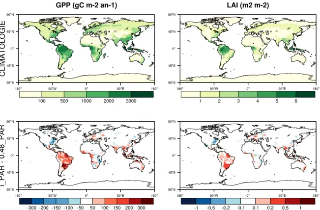
Figure C.1 – Impact du PAR interactif sur la GPP et le LAI en moyenne sur une p´eriode de 10 ans. Les panneaux du haut pr´esentent la climatologie, et les panneaux du bas repr´esentent l’anomalie entre la simulation utilisant le nouveau param`etre PAR interactif (i PAR) et la simulation utilisant la valeur fixe 0.48 (0.48 PAR).

flux brut de carbone, de l’atmosph`ere vers la biosph`ere. Le LAI (Leaf Area Index) repr´esente l’indice foliaire de la v´eg´etation, rapport entre la surface des feuilles de la plante et la surface de sol que couvre cette plante. Enfin, je pr´esente les cartes de temp´erature de surface et de pr´ecipitations.

Ce travail pr´eliminaire n´ecessite une ´evaluation compl`ete pour savoir s’il peut constituer un apport `a la mod´elisation du cycle du carbone. N´eanmoins, on peut noter la sensibilit´e des param`etres photosynth´etiques `a l’impl´ementation interactive de ce param`etre : l’impact sur l’Amazonie est significatif : augmentation de la GPP, du LAI, induisant un refroidissement local.

Enfin, notons que les valeurs de PAR simul´ees par le mod`ele s’´etendent entre 0.35 et 0.65, justifiant que la valeur 0.48 est bien trop restrictive au premier ordre. En effet, pour un rayonnement total incident identique entre deux points de grille, l’´energie r´eellement utilisable par la v´eg´etation peut varier du simple au double (pour des valeurs de PAR extrˆemes).

Figure C.2 – Impact du PAR interactif sur la TAS et les PR en moyenne sur une p´eriode de 10 ans. Les panneaux du haut pr´esentent la climatologie, et les panneaux du bas repr´esentent l’anomalie entre la simulation utilisant le nouveau param`etre PAR interactif (i PAR) et la simulation utilisant la valeur fixe 0.48 (0.48 PAR).

Comparaison des mod`eles

CNRM-ESM1 et CNRM-ESM2-1 :

cartes globales DJF et JJA des

champs de temp´erature, vent zonal

`a 850 hPa, et pr´ecipitations

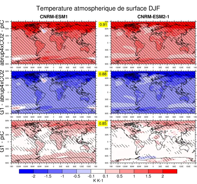
Figure D.1 – Anomalies de la temp´erature atmosph´erique de surface hivernale (DJF) entre les simulations G1, piControl et abrupt4×CO2 pour les mod`eles CNRM-ESM1 (`a gauche) et CNRM-ESM2-1 (`a droite). Pour chaque couple d’anomalies, la corr´elation spatiale entre les deux mod`eles est indiqu´ee sur fond jaune entre les deux panneaux. Les zones hachur´ees repr´esentent un niveau de significativit´e sup´erieur `a 90%, estim´e `a partir d’un test de Student sur l’´echantillon de 40 ann´ees.

d’anomalies, la corr´elation spatiale entre les deux mod`eles est indiqu´ee sur fond jaune entre les deux panneaux. Les zones hachur´ees repr´esentent un niveau de significativit´e sup´erieur `a 90%, estim´e `a partir d’un test de Student sur l’´echantillon de 40 ann´ees.

Figure D.3 – Anomalies du vent zonal `a 850 hPa en hiver (DJF) entre les simulations G1, piControl et abrupt4×CO2 pour les mod`eles CNRM-ESM1 (`a gauche) et CNRM-ESM2-1 (`a droite). Pour chaque couple d’anomalies, la corr´elation spatiale entre les deux mod`eles est indiqu´ee sur fond jaune entre les deux panneaux. Les zones hachur´ees repr´esentent un niveau de significativit´e sup´erieur `a 90%, estim´e `a partir d’un test de Student sur l’´echantillon de 40 ann´ees. La climatologie de la simulation de r´ef´erence est indiqu´ee en contours violets, par pas de 5 m.s-1_.

spatiale entre les deux mod`eles est indiqu´ee sur fond jaune entre les deux pan-neaux. Les zones hachur´ees repr´esentent un niveau de significativit´e sup´erieur `a 90%, estim´e `a partir d’un test de Student sur l’´echantillon de 40 ann´ees. La climatologie de la simulation de r´ef´erence est indiqu´ee en contours violets, par pas de 5 m.s-1_.

Figure D.5 – Anomalies des pr´ecipitations hivernales (DJF) entre les simulations G1, piControl et abrupt4×CO2 pour les mod`eles CNRM-ESM1 (`a gauche) et CNRM-ESM2-1 (`a droite). Pour chaque couple d’anomalies, la corr´elation spa-tiale entre les deux mod`eles est indiqu´ee sur fond jaune entre les deux panneaux. Les zones hachur´ees repr´esentent un niveau de significativit´e sup´erieur `a 90%, estim´e `a partir d’un test de Student sur l’´echantillon de 40 ann´ees.

tiale entre les deux mod`eles est indiqu´ee sur fond jaune entre les deux panneaux. Les zones hachur´ees repr´esentent un niveau de significativit´e sup´erieur `a 90%, estim´e `a partir d’un test de Student sur l’´echantillon de 40 ann´ees.