Identification of the accretion rate for annually resolved archives

(1)

HAL Id: hal-00297794

https://hal.archives-ouvertes.fr/hal-00297794

Submitted on 10 Apr 2006

HAL is a multi-disciplinary open access

archive for the deposit and dissemination of sci-entific research documents, whether they are pub-lished or not. The documents may come from teaching and research institutions in France or abroad, or from public or private research centers.

L’archive ouverte pluridisciplinaire HAL, est destinée au dépôt et à la diffusion de documents scientifiques de niveau recherche, publiés ou non, émanant des établissements d’enseignement et de recherche français ou étrangers, des laboratoires publics ou privés.

Identification of the accretion rate for annually resolved

F. de Ridder, A. de Brauwere, R. Pintelon, J. Schoukens, F. Dehairs

To cite this version:

F. de Ridder, A. de Brauwere, R. Pintelon, J. Schoukens, F. Dehairs. Identification of the accretion rate for annually resolved archives. Biogeosciences Discussions, European Geosciences Union, 2006, 3 (2), pp.321-344. �hal-00297794�

(2)

BGD

3, 321–344, 2006 Dating annually resolved archives F. De Ridder et al. Title Page Abstract Introduction Conclusions References Tables Figures J I J I Back Close

Full Screen / Esc

Printer-friendly Version

Interactive Discussion

EGU Biogeosciences Discuss., 3, 321–344, 2006

www.biogeosciences-discuss.net/3/321/2006/ © Author(s) 2006. This work is licensed under a Creative Commons License.

Biogeosciences Discussions

Biogeosciences Discussions is the access reviewed discussion forum of Biogeosciences

Identification of the accretion rate for

annually resolved archives

F. De Ridder1,2, A. de Brauwere2, R. Pintelon1, J. Schoukens1, and F. Dehairs2 1

Department of Fundamental Electricity and Instrumentation, Team B: System Identification and Parameter Estimation, Vrije Universiteit Brussel, Pleinlaan 2, 1050 Brussels, Belgium

2

Department of Environmental and Analytical Chemistry, Vrije Universiteit Brussel, Brussels, Belgium

Received: 22 November 2005 – Accepted: 9 January 2006 – Published: 10 April 2006 Correspondence to: F. De Ridder (federid@vub.ac.be)

(3)

BGD

Full Screen / Esc

EGU

Abstract

The past environment is often reconstructed by measuring a given proxy (e.g. δ18O) in an environmental archive, i.e. a species which gradually accumulates mass and records the current environment during this mass formation (e.g. corals, shells, trees, etc. . . ). When such an environmental proxy is measured, its values are known as

5

a function of distance. However, to relate the data to environmental variations, the date associated with each measurement, i.e. the time base, should be known. This is not straightforward solved, since species usually do not grow at constant rates. In this paper, we investigate this problem for annually resolved archives, which exhibit a certain periodicity. Such signals are often found in clams or corals. Due to variations

10

in accretion rate the data along the distance axis have a disturbed periodic profile. A method is developed to extract information about the accretion rate, such that the original (periodic) signal as function of time can be recovered. Simultaneously the exact shape of the periodic signal is estimated. The final methodology is quasi-independent of choices made by the investigator. Every step in the procedure is described in detail

15

and finally, the method is exemplified on a real world example.

1 Introduction

A problem often encountered in proxy-records is the reconstruction of the time-series, starting from measured distance series. Variations in accretion rate squeeze and stretch the distance series. This distortion results in the lengthening and shortening

20

of individual features present in the signal, a broadening of spectral peaks, as well as the appearance of extraneous spectral peaks (see e.g. De Ridder et al., 2004). Such a distortion may occur during the recording (natural or artificial) of a signal or during its passage through certain kinds of filtering media. In some cases the accretion rate itself is of more interest than the recovered signal. In other cases it may be of interest

25

(4)

BGD

Full Screen / Esc

EGU by correlating by eye. This, however, works only in the simplest cases, is not readily

quantified and is generally limited to low resolution. What makes things worse is that two investigators, who are dating the same record with such an identical method, will come to different conclusions, because they may have selected different tuning points. In the early ’80s Martinson et al. (1982) proposed an inverse approach to signal

cor-5

relating. They have presented a quantitative method for correlating a distance series with a given time series. In this paper, we go one step further and will estimate not only the accretion rate, but also the shape of the time series. To do so, we had to assume that the “true” time series is periodic. A second difference is that an automated model selection procedure is implemented, which chooses the model complexity using more

10

objective, statistical rules. As will be shown, this allows us to extract the maximum amount of significant information from noisy data.

For the scope of this paper, we have assumed that when a measured proxy record is compared with a model, three types of errors occur:

1. Stochastic noise: models and data will never match perfectly. This has two

rea-15

sons: (i) the measurements are disturbed by an unknown number of small effects, like instabilities in the measurement instrument etc. . . , and (ii) the modeled sys-tem can have a chaotic component. Fortunately, both effects can quite easily be described by an additional stochastic component in the model expression.

s_n = s_model(t_n)+ e (1)

20

where n is the sample number, s the measured signal, s_model the model, t_n the date of observation n and e the error term, describing the difference between measurements and model. The main characteristics of this component are that it is zero on the average and that it can usually be described by a normal distribution with a standard deviation, σ.

25

Stochastic errors can be reduced by

(5)

BGD

Full Screen / Esc

EGU (ii) repeated measurements, which is time consuming. Here the model and

sys-tematic errors are deterministic and will be identical in each measurement set, while the stochastic errors will differ from measurement set to measure-ment set and can thus be averaged out;

(iii) a parametric model, which can introduce additional model errors. The

5

stochastic errors inherent in each measured sample will average out when the parameters are estimated. The improved precision is mainly determined by the ration measured observation to number of parameters.

2. Model errors are non-stochastic components that are not described by the model and which are not hidden by the stochastic noise. Identifying these is possible

10

only after analyzing the stochastic properties. Systematic errors can occur due to inaccurate measurements or by un-modeled effects in the studied system and can thus be avoided by improving the accuracy of the measurement or by refining the model.

3. A special type of systematic errors, which is specific for proxy records and

sedi-15

ment analysis are dating errors (Martinson et al., 1982; Paillard et al., 1996; Yu and Ding, 1998; Lisiecki and Lisiecki, 2002; Ivany and Wilkinson, 2003). In the scope of this paper, these are catalogued as a separated third class. In this paper a strategy to remove this type of errors systematically is proposed, by refining the model.

20

The methodology proposed is based on the next remarks: in the measurement set the values of the observations are given, but the corresponding dates are missing. On the other hand, we often have a model, containing time. However, notice that each model consists of some model parameters, which can only be tuned by matching the model on the measurement set. So, in this context neither

25

the experimentalist, nor the modeler has enough information to work isolated. Here, both are combined. The focus is on annually resolved archives, which often have a clear periodic component, so the discussion can be limited to periodic

(6)

BGD

Full Screen / Esc

EGU signal models. Still, in general even climate models (Martinson et al., 1982) or

other signal models1 can be used. First the signal and time base models are explained and next solutions are given for two particular problems, i.e.

(i) gathering initial values for the parameters; and

(ii) due to the parametric representation of the time base, neighboring

observa-5

tions can be altered, which would mean that the time is locally inverted. This artifact is circumvented.

The approach is finally illustrated on two proxy records measured in clams.

2 The signal and time base model

In this and the next paragraph the formal set-up of the methodology (i.e. the equations

10

used) are briefly explained. The signal under investigation is assumed to be periodic, sampled along an equidistant distance grid. Formally, this translates to the assumption that the discrete-time signal, s_model(t_n), is given by

s_model(t_n)= A₀+

h X k=1

A_kcos(kωt_n)+A_k_+hsin(kωt_n) (2)

where t_n is the unknown time variable at sample position, n ∈ {1, . . . , N}, A₀ the o

ff-15

set, A_k and A_k_+h are the unknown amplitudes of the kth harmonic, ω is the unknown fundamental angular frequency and h the number of harmonics, yet to be identified. Changing the number of harmonics will change the complexity of the model (Fig. 1). Although the samples are equidistantly spaced along the distance axis, the time in-stance between two subsequent samples is not constant, because of variations in the

20

1

A signal model is a black box or empirical (versus physical) model describing the variation of the proxy, e.g. a sinusoidal or polynomial model.

(7)

BGD

Full Screen / Esc

EGU accretion rate. These distortions of the time base are modeled by a function, δ_n, called

the time base distortion (T.B.D.)

δ_n =

b X m=1

B_mφ_m(n) (3)

where φ is a set of b basis functions, B is a vector of length b, yet to be identified, with the unknown time base distortion parameters. The parameter b defines the complexity

5

of the time base (vide infra). Note that it is practically impossible to estimate the time base distortion directly, by comparing the measurements with the signal model (Eq. 2), because

(i) the measured record is disturbed by stochastic noise, which would be propagated into the time base distortion; and

10

(ii) the signal model’s parameters and complexity are unknown (so we can only as-sume that it is periodic, without knowing its precise shape).

The first problem is circumvented by the introduction of basis functions. We have tested trigonometric functions, Legendre polynomials and splines as basis function (Abramowitz and Segun, 1968; Dierckx, 1995). The latter seems to work best.

15

The time instances, t_n, are given by

t_n= (n + δ_n)T_s (4)

where T_s is the average sample period.

In order to overcome the second problem, all the unknowns, the model parameters and the time base distortion, are represented by some unknown parameters. For fixed

20

values of h and b, these can be grouped in a vector

θ= [ω, AT, BT]T (5)

The optimal set of parameters can be calculated by a numerical minimization algorithm, which minimizes a least squares cost function. For this task a Levenberg-Marquardt algorithm was implemented (e.g. Pintelon and Schoukens, 2001).

(8)

BGD

Full Screen / Esc

EGU

3 Starting value problem and optimization strategy

Minimizing this cost function will only be successful, if one can start from a reasonable set of initial values. Otherwise the local optimization method will possibly not be able to converge towards a good minimum. In order to minimize the risk of converging towards a bad local minimum, the optimization strategy is performed in five steps (for a structure

5

of the algorithm, see Fig. 2):

1. Initializing the frequency, ω: a non-parametric time base distortion and the cor-responding frequency can be gathered for periodic signal records, following the guidelines of (De Ridder et al., 2004);

2. Initialization of the T.B.D. parameters, B: initial values for the T.B.D. parameters

10

can be gathered by matching Eq. (3) on the non-parametric T.B.D. This can easily be done, because Eq. (3) is linear in the parameters, B. Next, Eq. (4) is used to get more precise dates of the observations.

3. Initialization of the signal parameters, A: these are gathered by matching Eq. (2) on the observations employing the previously estimated time base. An efficient

15

algorithm is described in (Pintelon and Schoukens, 1996).

4. Relaxation: alternating, the T.B.D. parameters and the signal parameters are op-timized, while the other set is remained fixed. Note that optimizing the T.B.D. pa-rameters, while the signal parameters are constant is, in fact, the parametric or-bital tuning method proposed by Martinson et al. (1982). This relaxation algorithm

20

is stopped when the largest relative variation in the parameter vector, θ, is lower than a numerical stop criterion (typically 10−3). This step in the optimization is implemented to increase the calculation speed but it will not influence the final results.

5. Final estimation of parameters: all parameter values are estimated together

em-25

(9)

BGD

Full Screen / Esc

EGU

4 Local time reversal problem

The method seems to have a major weakness: it is sensitive to time reversal problems, especially when the number of time base distortion parameters is relatively high (an example is given in Fig. 3). This is not surprising, because the noise sensitivity is larger in this case. However, we know that such time reversals are physically impossible,

5

so the algorithm has to be extended: to avoid this unrealistic behavior an inequality constraint optimization was implemented (e.g. Fletcher, 1991): in each step of the Levenberg-Marquardt algorithm a check is performed to verify if any time reversals have occurred: is the minimal sample period lower than 20% of the average sample period? If so, the constraints become active and the time base distortion at these

10

samples is fixed at this minimum for this step of the optimization routine. The dotted line in Fig. 3 shows the result after the implementation of the inequality constraint optimization.

5 Model selection criterion

If we would stop developing the algorithm at this point, the complexity of the signal

15

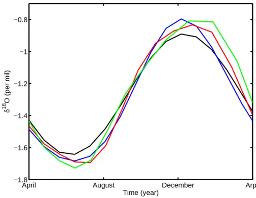
model and time base model, quantified by h and b, respectively, are still chosen by the user. Figure 4 shows the accretion rate and Fig. 5 the signal models, estimated from the same measurement record, with identically the same algorithm, but with different levels of complexity. So, two types of problems can occur:

(i) if two investigators would process the same record with the same algorithm and

20

based on the same assumptions, it is still possible that they come to different conclusions;

(ii) Maybe the true time base and/or signal models are more complex than defined by the investigator. This would mean that not all useful information is extracted from

(10)

BGD

Full Screen / Esc

EGU the data. On the other hand is the risk also present that the chosen complexity

was too high. This would result in conclusions that are not supported by the data. What is happening? And can we do anything about it? The fact that the model and time base parameters can be optimized does not tell us anything about the significance of these parameters. It is very well possible that e.g. too much time base parameters

5

are used, which would all be insignificant. These redundant parameters are only used to model the measurement noise. In this paragraph we tell how to find the optimal values for the number of harmonics, h, and for the number of T.B.D. parameters, b. To begin, we define the model complexity by the number of parameters, which are opti-mized. Increasing the model complexity will decrease the systematic errors, however,

10

at the same time the model variability increases2. Hence, it is not a good idea to se-lect the model with the smallest cost function within the set because it will continue to decrease when more parameters are added. At a certain complexity the additional parameters no longer reduce the systematic errors but are used to follow the actual noise realization on the data. As the noise varies from measurement to measurement,

15

the additional parameters increase only the model variability. However, usually we do not have repeated measurements and we would still like to draw conclusions from a model. For this reason, the cost function is extended with a model complexity term that compensates for the increasing model variability. Summarized, the model selection cri-terion, called MDL_c3, should be able to detect undermodeling (= too simple model) as

20

well as overmodeling (= too complex model). This model complexity term is dependent upon the signal-to-noise ratio and the availability of a noise model. In the examples of

2

This means that if one would redo the measurement and match the same model, with the same model complexity again, the difference between the old and new model will be larger.

3

We have followed the “minimum description length” nomenclature proposed by Rissanen (1978), which is also called the BIC criterion (Schwartz, 1978).

(11)

BGD

Full Screen / Esc

EGU this paper the criterion to be minimized had the following expression

MDL_c( ˆθ, n_θ, n_c, N)= K ( ˆθ)

N exp pc(nθ, nc, N) (6)

with penalty p_c(n_θ, n_c, N)= ln(N)(nθ− nc+ 1) N− (nθ− nc) − 2

with K ( ˆθ) the residual cost function, N the total number of observations and n_θ the number of parameters, reduced by the number of active constraints, n_c. Notice that

5

introducing a model selection criterion eliminated interferences from the user, which makes the proposed method more objective and user independent.

Practically, the user chooses the maximum values for h and b, i.e. (h, b)_max. Next, all models with a model complexity from (h, b)=(0, 0) till this maximum are optimized and Eq. (8) is used to select the best model within this set (lowest MDL_cvalue). A detailed

10

description of the model selection criteria can be found in (Akaike, 1974; Rissanen, 1978; Schwartz, 1978; De Ridder et al., 2005, de Brauwere et al., 2005).

6 Application: saxidomus giganteus

As an example, the δ18O-signals measured in Saxidomus giganteus are processed. Two specimens were sampled from the West coast of the USA in Washington state,

15

named Clam 1 and Clam 2. The large winter-summer variations are reflected in these signals (Figs. 6a and 7a) and this periodicity will be used to date the observations. The two clams lived under identical environmental conditions, so the correlation between the signals can be used to validate the method. In addition, the estimated accretion rates are compared.

20

To test the algorithm, the maximum model complexity was limited to (h, b)_max=(4, 20), i.e. four harmonics can be used to describe the signal model and 20 parameters can be used for the time base distortion. For some model complexities,

(12)

BGD

Full Screen / Esc

EGU the constraints became active. This was mostly the case when the number of time

base distortion parameters, b, became high. The results are summarized in Table 1: the lowest model selection criteria, MDL_c, values were twice found for a signal model consisting of only one harmonic (see Figs. 6 and 7). Both samples were collected in 2001 and the most recent observation was dated as 1 April, so that annual maxima

5

in δ18O correspond to winter situations. The corresponding correlation between both

records is 84% (see Fig. 8).

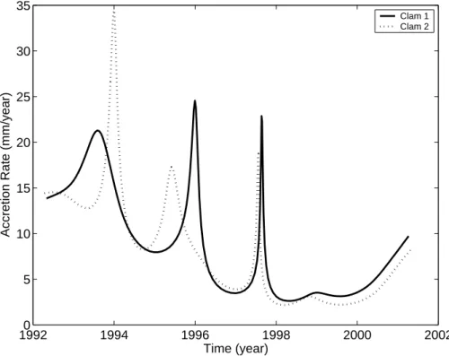
The accretion rates of both clams are shown in Fig. 9. Note that

1. Maybe annual variations in the accretion rate did occur, but such a time base distortion model was too complex according to the model selection criteria. So,

10

the quality of the data is not sufficient to support annual variations in the time base distortion;

2. The estimated accretion rates decrease slowly with age, which can be expected; 3. most variation occurs at more or less the same moments in both clams. This is

reflected in the correlation of 63% between the two accretion rate profiles. The

15

mismatch between the two peaks around 1996 can be due to errors still present in the time base, which is used to construct and date the accretion rate. An alternative explanation can be found in the fact that the accretion rate is a non-linear function of the time base distortion parameters. Consequently, small errors on these parameters can have a large influence on the accretion rate than on the

20

time base distortion itself.

The relatively high correlation illustrates that these variations are relevant (do not reflect the stochastic noise) and that they are determined not only by the age of the spec-imens, but also by external forcing. Otherwise, accretion rate would decrease much smoother with age or in a random manner. Such precise estimations of the accretion

25

(13)

BGD

Full Screen / Esc

EGU

7 Conclusion

We have presented a new method to reconstruct the time base for periodic archives. It is based on (Martinson et al., 1982) and (De Ridder et al., 2004). The novelty of this approach is that it estimates the time base together with the signal, describing the time series. The method is build around an identification approach and which has several

5

advantages:

(i) it is combined with a statistically-based model selection criterion, to choose the most appropriate model complexity;

(ii) which makes it is robust to overmodeling in the signal and time base model; and (iii) which makes it robust to undermodeling;

10

(iv) it is robust to stochastic measurement errors, since parametric signal and time base models are used,

(v) it is robust to non-sinusoidal periodic signals, because overtones are modeled too.

The combination of (i), (iv) makes it possible to separate largely the stochastic noise

15

from the significant variations. The combination of (i), (ii) and (iii) allows the user to extract the maximum amount of significant information, hidden in the record. In addition all tuning is done by the algorithm, which makes the method user-friendly and more objective. On the other hand, the algorithm does assume that the “true” record is periodic, which may not be true. A violation of this assumption may bias the final result.

20

Note that the strategy proposed here is not limited to this specific periodic signal model, although gathering initial values for arbitrary models can become a hard task.

The method has been exemplified on two records of δ18O, measured in clams. Both clams lived in the same environment, so the time series of δ18O could be used to check the robustness of the method. After optimization, the correlation between both records

(14)

BGD

Full Screen / Esc

EGU was 84%. Furthermore, the correlation between the independently estimated accretion

rates was 63%. This could indicate that also the accretion rate is changing with varying environmental conditions in a deterministic manner.

A matlab version of the algorithm is available on request.

Acknowledgements. F. De Ridder and A. de Brauwere are researcher of the Flemish Fund 5

for Scientific Research (FWO-Vlaanderen) and are grateful for their support. This work was also supported by the Belgian Government (IUAP V/22), the Flemish Government and the Vrije Universiteit Brussel (GOA22/DSWER4, GOA23-ILiNoS, and HOA9). We are grateful to D. P. Gillikin for providing data from the Saxidomus giganteus clams. Finally, we would like to thank G. Munhoven and D. Paillard for their comments and critics on this work.

10

References

Abramowitz, M. and Segun, I. A.: Handbook of Mathematical Functions with Formulas, Graphs, and Mathematical Tables, New York, Dover, 1968.

Akaike, H.: A new look at the statistical model identification, IEEE T. Automat Contr., AC-19, 716–723, 1974.

15

de Brauwere, A., De Ridder, F., Pintelon, R., Elskens, M., Schoukens, J., and Baeyens, W.: Model selection through a statistical analysis of the minimum of a Weighted Least Squares cost function, Chemometr. Intell. Lab., 76, 163–173, 2005.

De Ridder, F., Pintelon, R., Schoukens, J., Gillikin, D. P., Andr ´e, L., Baeyens, W., de Brauwere, A., and Dehairs, F.: Decoding nonlinear growth rates in biogenic environmental archives,

20

Geochem. Geophy. Geosy., 5(12), Q12015, doi:10.1029/2004GC000771, 2004.

De Ridder, F., Pintelon, R., Schoukens, J., and Gillikin, D. P.: Modified AIC and MDL model selection criteria for short data records, IEEE T. Instrum. Meas., 54(1), 144–150, 2005. Dierckx, P.: Curve and surface fitting with splines, Oxford Univ. Press, 1995.

Fletcher, R.: Practical methods of optimization, John Wiley and Sons Ltd., Chichester, 1991.

25

Golub, G. H. and Van Loan, C. F.: Matrix Computations, Johns Hopkins University Press, Baltimore, MD, 1990.

(15)

BGD

Full Screen / Esc

EGU duration of growth throughout ontogeny: an example from the Surf Clam, Spisula solidissima,

Palaios, 18, 126–137, 2003.

Lisiecki, L. E. and Lisiecki, P.: Application of dynamical programming to the correlation of pale-oclimate records, Paleoceanography, 17(D4), 1049–1061, 2002.

Paillard, D., Labeyrie, L., and Yiou, P.: Macintosh program performs time-series analysis, Eos

5

Transactions AGU, 77(39), 379, 1996.

Martinson, D. G., Menke, W., and Stoffa, P.: An inverse approach to signal correlation, J. Geophys. Res., 87(B6), 4807–4818, 1982.

Pintelon, R. and Schoukens, J.: An improved Sine-Wave Fitting Procedure for Characterizing Data Acquisition Channels, IEEE T. Instrum. Meas., 45(2), 588–593, 1996.

10

Pintelon, R. and Schoukens, J.: System Identification A Frequency Domain Approach, IEEE PRESS, New York, 2001.

Rissanen, J.: Modeling by shortest data description, Automatica, 14, 465–471, 1978. Schwarz, G.: Estimating the dimension of a model, Ann. Stat., 6(2), 461–464, 1978.

Yu, Z. W. and Ding, Z. I.: An automatic orbital tuning method for paleoclimate records, Geophys.

15

(16)

BGD

Full Screen / Esc

EGU

Table 1. Summary of the selected models used in the Saxidomus giganteus examples.

Clam 1 Clam 2 Residual cost function (per mil)2, K ( ˆθ) 3.48 4.64 Automated model selection criterion (per mil)2, MDLc 0.045 0.048

Number of observations, N 133 123

Selected number of harmonics, h 1 1

(17)

BGD

Full Screen / Esc

EGU

0 1 2 3

Signal (No Units)

Time domain

0 1 5 10

Frequency domain

0 1 2 3 Amplitude (no units)0 1 2 5 10

0 1 2 3

Time (e.g. year)

0 1 2 3 4 5 10

Frequency (e.g. 1/year) h=1

h=2

h=5

Fig. 1. Several signals are shown in the time and frequency domain. All signals are periodic,

which is best seen in the frequency domain: the only non-zero amplitudes are found at integer frequencies. Notice further that with only one harmonic, h=1, the time signal is sinusoidal, while more complex periodic signals can be described using multiple harmonics.

(18)

BGD

Full Screen / Esc

Printer-friendly Version Interactive Discussion EGU INITIALISATION RELAXATION LEVENBERG-MARQUARDT SET OF ALL OPTIMIZED MODELS frequency signal parameters time base signal parameters TBD parameters i ˆ Ǉ ... ... i ˆ_Ǉ 1 ˆ Ǉ ˆǇ2 ˆǇmax

AUTOMATED MODEL SELECTION

ˆ Ǉ

(19)

BGD

Full Screen / Esc

Printer-friendly Version Interactive Discussion EGU 20 25 30 35 40 45 50 0.5 1 1.5 2

Distance from Umbo (mm)

Time (year)

Fig. 3. Around 35 mm from the Umbo, the estimated time is constant (full line), which would

correspond to an infinite accretion rate. In order to avoid this type of un-physical solutions, an inequality constraint optimization is implemented: if negative accretion rates occur, the time base is forced to remain slightly positive (dotted line).

(20)

BGD

Full Screen / Esc

Printer-friendly Version Interactive Discussion EGU 0 1 2 3 4 5 6 7 8 9 0 10 20 30 40 50 60 70 80 Time (year)

Accretion Rate (mm/year)

Fig. 4. The accretion rates are shown for different sets of model complexity (all matched on

clam 1 (vide infra)): in black (h=1, b=5), in blue (h=2, b=10), in red (h=3, b=15) and in green (h=4, b=20). The variations increase with increasing complexity, but so far, we are not able to tell which of these accretion rates describes best reality. Note that the accretion rate of about 70 mm/year for the two most complex models is fixed at these levels due to the constraints, which have become active.

(21)

BGD

Full Screen / Esc

EGU

April August December Arpil

−1.8 −1.6 −1.4 −1.2 −1 −0.8 Time (year) δ 18 O (per mil)

Fig. 5. One period of the periodic signals is shown (matched on clam 1 (vide infra)): in black

(h=1, b=5), in blue (h=2, b=10), in red (h=3, b=15) and in green (h=4, b=20). Note that the amplitude of the black signal is different from that of the green signal. Further, the minima of the signals correspond quite well (June), but the maxima changes with about one month. Which of these models is closed to reality?

(22)

BGD

Full Screen / Esc

Printer-friendly Version Interactive Discussion EGU 10 20 30 40 50 60 70 80 90 100 −2.5 −2 −1.5 −1 −0.5 0 0.5

δ 18 0 (per mil) 1992 1994 1996 1998 2000 2002 −2.5 −2 −1.5 −1 −0.5 0 0.5 Time (year) δ 18 0 (per mil) (a) 10 20 30 40 50 60 70 80 90 100 −2.5 −2 −1.5 −1 −0.5 0 0.5

δ 18 0 (per mil) 1992 1994 1996 1998 2000 2002 −2.5 −2 −1.5 −1 −0.5 0 0.5 Time (year) δ 18 0 (per mil) (b) Fig. 6. Clam 1: (a) raw data and (b) signal on the constructed time base (full line) and the

(23)

BGD

Full Screen / Esc

Printer-friendly Version Interactive Discussion EGU 10 20 30 40 50 60 70 80 90 100 −2.5 −2 −1.5 −1 −0.5 0 0.5

δ 18 0 (per mil) 1992 1994 1996 1998 2000 2002 −2.5 −2 −1.5 −1 −0.5 0 0.5 Time (year) δ 18 0 (per mil) (a) 10 20 30 40 50 60 70 80 90 100 −2.5 −2 −1.5 −1 −0.5 0 0.5

δ 18 0 (per mil) 1992 1994 1996 1998 2000 2002 −2.5 −2 −1.5 −1 −0.5 0 0.5 Time (year) δ 18 0 (per mil) (b) Fig. 7. Clam 2: (a) raw data and (b) signal on the constructed time base (full line) and the

(24)

BGD

Full Screen / Esc

Printer-friendly Version Interactive Discussion EGU 1992 1993 1994 1995 1996 1997 1998 1999 2000 2001 2002 −2.5 −2 −1.5 −1 −0.5 0 0.5 Time (year) δ 18 0 (per mil) Clam 1 Clam 2

(25)

BGD

Full Screen / Esc

Printer-friendly Version Interactive Discussion EGU 19920 1994 1996 1998 2000 2002 5 10 15 20 25 30 35

Accretion Rate (mm/year)

Time (year)

Clam 1 Clam 2