HAL Id: hal-00316846
https://hal.archives-ouvertes.fr/hal-00316846
Submitted on 1 Jan 2001
HAL is a multi-disciplinary open access
archive for the deposit and dissemination of
sci-entific research documents, whether they are
pub-lished or not. The documents may come from
teaching and research institutions in France or
abroad, or from public or private research centers.
L’archive ouverte pluridisciplinaire HAL, est
destinée au dépôt et à la diffusion de documents
scientifiques de niveau recherche, publiés ou non,
émanant des établissements d’enseignement et de
recherche français ou étrangers, des laboratoires
publics ou privés.
southern polar cap from ground-based vertical velocity
and photometric observations
J. L. Innis, P. A. Greet, P. L. Dyson
To cite this version:
J. L. Innis, P. A. Greet, P. L. Dyson. Evidence for thermospheric gravity waves in the southern
polar cap from ground-based vertical velocity and photometric observations. Annales Geophysicae,
European Geosciences Union, 2001, 19 (5), pp.533-543. �hal-00316846�
Annales Geophysicae (2001) 19: 533–543 c European Geophysical Society 2001
Annales
Geophysicae
Evidence for thermospheric gravity waves in the southern polar cap
from ground-based vertical velocity and photometric observations
J. L. Innis1, P. A. Greet1, and P. L. Dyson21Australian Antarctic Division, Kingston, Tasmania, 7050, Australia 2La Trobe University, Bundoora, Victoria, 3083, Australia
Received: 27 November 2000 – Revised: 20 February 2001 – Accepted: 18 March 2001
Abstract. Zenith-directed Fabry-Perot Spectrometer (FPS)
and 3-Field Photometer (3FP) observations of the λ630 nm emission (∼240 km altitude) were obtained at Davis sta-tion, Antarctica, during the austral winter of 1999. Eleven nights of suitable data were searched for significant period-icities common to vertical winds from the FPS and photo-metric variations from the 3FP. Three wave-like events were found, each of around one or more hours in duration, with periods around 15 minutes, vertical velocity amplitudes near 60 m s−1, horizontal phase velocities around 300 m s−1, and horizontal wavelengths from 240 to 400 km. These charac-teristics appear consistent with polar cap gravity waves seen by other workers, and we conclude this is a likely interpre-tation of our data. Assuming a source height near 125 km altitude, we determine the approximate source location by calculating back along the wave trajectory using the gravity wave property relating angle of ascent and frequency. The wave sources appear to be in the vicinity of the poleward bor-der of the auroral oval, at magnetic local times up to 5 hours before local magnetic midnight.
Key words. Meteorology and atmospheric dynamics
(ther-mospheric dynamics; waves and tides)
1 Introduction
Generation of atmospheric gravity waves in or near the au-roral electrojets is well documented. Early evidence of iono-spheric waves travelling from the polar regions (e.g. Heisler, 1958; Munro, 1958; Georges, 1968; Testud and Vasseur, 1969), and theoretical studies (e.g. Chimonas and Hines, 1970; Richmond, 1978) have been followed by further ob-servations and interpretation (such as Spencer et al., 1976; Hernandez and Roble, 1978; Chandra et al., 1979; Crowley and Williams, 1987; Williams et al., 1988, 1993; Bristow et al., 1994, 1996; Lewis et al., 1996; Ma et al., 1998), includ-ing consideration of the consequences for the thermal
struc-Correspondence to: J. L. Innis (john.innis@aad.gov.au)
ture and dynamics of the atmosphere due to the waves (e.g. Richmond and Roble, 1979). Reviews by Francis (1975) and Hunsucker (1982) discuss early work, while Hocke and Schlegel (1996) outline results obtained from 1982 to 1996.
Optical studies also revealed evidence for gravity waves with auroral sources. Herrero et al. (1984) using a Fabry-Perot Spectrometer (FPS) observed wave-like vertical veloc-ity and temperature fluctuations in oxygen λ630 nm emission data (∼240 km altitude) at high northern latitudes, which appeared consistent with their model of a heating source at 120 km altitude. Rees et al. (1984a) showed large amplitude (100–200 m s−1), thermospheric vertical winds occur on the poleward edge of the auroral oval. Rees et al. (1984b) con-sidered the implications of these data for the generation of gravity waves.
De Deuge et al. (1994) conducted a long-term photomet-ric study over Mawson station, Antarctica, at both λ630 nm (from ∼240 km altitude) and λ558 nm (from ∼120 to 150 km altitude) wavelengths. Waves seen at λ630 nm preferentially propagated to the magnetic north of the station, with a smaller number propagating magnetic south. They accounted for this assuming that the auroral oval (the likely source of the waves) generates both poleward- and equatorward-travelling waves. At intervals of low to moderate activity the oval is mostly poleward of Mawson. During high-magnetic activ-ity, the oval may be equatorward of Mawson for an extended time. This allowed the detection of some magnetically-south directed waves.
Gravity waves in the polar cap thermosphere were seen in Dynamics Explorer–2 satellite data by Johnson et al. (1995). Fifty-one waves were detected, with typical vertical veloc-ity amplitudes of around 100 m s−1, periods around 1000 s, and they appeared to travel from the night- to the day-side. Fifteen polar cap waves were observed by MacDougall et al. (1997), using digital ionosonde data from three northern high-latitude sites, with properties comparable to those seen by Johnson et al. (1995) when differences in observational techniques were taken into account.
to detect equatorward travelling F-region gravity waves and found the source locations were on the poleward side of the auroral oval, at least during intervals of low magnetic activ-ity, when their ground-scatter observations were possible.
Innis et al. (1997, 1998) suggested the source of polar cap waves may be linked to thermospheric upward winds at the poleward edge of the auroral oval, and that wave dissipation could heat the high-latitude thermosphere. Large upward winds, up to 100 to 200 m s−1, were seen first in F-region DE-2 spacecraft data by Spencer et al. (1982) at auroral lat-itudes. Price et al. (1995) observed simultaneous upwellings in the lower and upper thermosphere (∼150 and ∼240 km altitude) on the poleward edge of the northern auroral oval, noting the upwellings were most likely due to the advec-tion of an existing region of upward winds into the instru-ment field of view. FPS λ630 nm observations by Innis et al. (1996, 1997) indicate upward winds commonly appear in the high-latitude thermosphere from a region poleward of the oval near local magnetic midnight. Using data from two Antarctic stations, separated by about 800 km, Innis et al. (1999) tracked over several hours a region of upward wind some 6 × 10¹¹m2in areal extent.
Diurnal and seasonal variations of thermospheric vertical motions have been considered by Aruliah and Rees (1995), Conde and Dyson (1995), and Smith and Hernandez (1995). Smith (1998) reviewed thermospheric vertical winds.
In 1999, we conducted observations at Davis station, Ant-arctica (geog. long. = 78.0◦ E, lat. = −68.6◦ S; invariant lat. = −74.6◦ S). Our aim was to look for the presence of thermospheric gravity waves over Davis station. We used an FPS to observe the λ630 nm oxygen emission in the vertical direction in several campaigns during the austral winter, to-gether with a multi-channel three-field photometer (3FP). We expected any thermospheric gravity waves would be revealed by vertical velocity motions in the FPS data, correlated with photometric variations in the 3FP observations. Section 2 of this paper presents a brief description of the data sets, meth-ods of reduction, and some example data. Section 3 gives details of the analysis techniques used to search for waves in the data. Results are given in Sect. 4, with a discussion of our findings in Sect. 5.
2 Experimental details
2.1 The FPS
The Davis FPS is similar in design and operation to the FPS at Mawson station, which is described by Jacka (1985). Ob-servations of a frequency-stabilised HeNe laser are used to derive the instrumental profile, while regular observations of a neon hollow-cathode lamp are used to correct for instru-mental drift. The etalon spacing was chosen so that con-tamination from sky lines from the hydroxyl molecule at λ629.799 nm and λ630.683 nm was avoided (see Innis et al., 1999). The full-angle field-of-view of the FPS was set to 0.5◦.
Three zenith-direction observing campaigns were run in 1999: 1 March to 15 April; 1 July to 15 August; and 1 September to 20 October. In the first campaign, and for the first few days of the second, one sky/neon lamp observation was obtained approximately every 420 seconds during the night. From 13 July the wavelength range scanned was re-duced to improve the time resolution, giving a cycle time of 210 seconds from this date onwards.
Raw λ630 nm sky profiles were processed to yield ver-tical winds (velocities), temperatures, and relative intensities by deconvolving the instrument function from each sky spec-trum, and then fitting a Gaussian function. (Instrumental ef-fects, such as the photomultiplier dark count, are also taken into account.) The wind, temperature, and relative inten-sity are found from the Gaussian peak position, width, and area under the curve, respectively. Uncertainties in the fitted quantities give an estimate of the observational errors. We show wind and intensity data here, and will briefly mention temperature data when relevant.
A long-standing difficulty with FPS λ630 nm oxygen au-roral/airglow observations is that the zero velocity position is extremely hard to determine, as a reference λ630 nm oxy-gen laboratory source was not available. We adopt the usual approach and determine a zero from the mean zenith wind taken over a given observing night. Aruliah and Rees (1995) concluded that this can lead to errors of the order of 5 m s−1 at geomagnetically quiet times, and up to 10 m s−1during intervals of increased activity.
2.2 The 3FP
The 3FP is described in De Deuge et al. (1994). Three circu-lar fields of diameters 3.3◦, centred on the zenith and offset from it by 4.7◦, are sequentially observed through four dif-ferent filters: λ428 nm, λ558 nm, λ630 nm, and λ730 nm. Each observation through a given filter is 2.5 seconds in du-ration, and a complete cycle running all filters through each field takes 40 seconds.
Data analysis involves resampling the data strings (via the Fourier shift theorem) from each field to a common time ori-gin. Data at times of bright aurora are rejected. A cross-spectral analysis of all three fields is performed on selected time intervals to look for the presence of common signals. Phase lags between each field indicate the direction of wave motion (see De Deuge et al., 1994, for more details). 2.3 The data
In the three zenith campaigns, the FPS was operated every night when there was no falling snow or high wind. Approx-imately 70 nights of data were obtained. We have selected intervals where the maximum amount of recorded cloudiness was 2/8 or less, giving a set of 21 nights. (An all-sky Auroral Imager, AI, observing at λ558 nm, was operated each night. These images assisted significantly in identifying cloud-free intervals, and in tracking the movement and form of auroral displays.)
J. L. Innis et al.: Thermospheric gravity waves in the southern polar cap 535
Fig. 1. FPS λ630 nm data of wind and relative intensity from DoY 255.
We see a variety of behaviour in the vertical winds on dif-ferent nights. We present four nights of data to illustrate some of these features, and show what we interpret as wave records on three of these nights. Figures 1, 2, 3 and 4 show the wind (upper panel), and relative intensity (lower panel) time series measured from the oxygen λ630 nm emission profiles on the nights of Day of Year (DoY) 255, DoY 111, DoY 202, and DoY 220, respectively, which are briefly de-scribed here.
2.3.1 DoY 255
(Ap = 31, Fig. 1). During times of moderate overhead aurora, the vertical winds are generally near zero. At intervals when the aurora is northward of Davis, we see evidence for upward (positive) winds (e.g. ∼20:30 UT). A large event occurs in the vertical wind near 22 UT, with firstly an upward wind near 150 m s−1(seen in adjacent data points), followed by a
downward wind of nearly the same magnitude some 30 min-utes later, with a smaller upward wind (∼70 m s−1) about 20 minutes after that. Such large upward (and downward) winds appear identical with the winds seen over Mawson and Davis stations, and elsewhere, poleward of the auroral oval (e.g. Innis et al., 1996, 1997, 1999). We discuss below why we believe this is not the signature of an atmospheric grav-ity wave, although it is possible that these upward winds just poleward of the auroral oval may produce, or be linked to
processes that produce such waves (e.g. Rees et al., 1984a,b; Innis et al., 1997).
2.3.2 DoY 111
(Ap = 12, Fig. 2). There was relatively little overhead aurora, apart from the start and end of the night. AI images confirm Davis was in the polar cap for most of the night. Of particular relevance here are the wind data points around 18:30-20 UT, which have the appearance of an oscillation, with a time-scale near 20 to 30 minutes and amplitude around 50 m s−1, to be discussed in the next section.
2.3.3 DoY 202
(Ap = 14, Fig. 3). Data from this night show wave-like os-cillations in the wind during two clear-sky intervals. The first, near 17 UT, shows several up/down cycles of ampli-tude around 50 m s−1, with a period near 1000 s (5 data points). The second, from ∼21 to ∼23 UT, shows a similarly sized oscillation, but with a longer period, with the sugges-tion that the period decreases during the event. AI images from both instances indicate clear sky conditions, although overhead clouds probably resulted in or contributed to the large zenith winds at ∼20 UT when the aurora was overhead. From the start of the wave-like event at ∼21:15 UT onwards, the aurora was well to the equatorward of the zenith, and at
Fig. 2. FPS λ630 nm data of wind and relative intensity from DoY 111.
times, over the Davis horizon. As discussed later, the ∼21 to ∼23 UT event may be the signature of a gravity wave.
A revision in the adopted zero level by about 50 m s−1
could change the 21–23 UT event into a series of upward wind events. The run of high positive velocities near 20 UT may give the appearance of depressing the derived zero mean calculated over the whole night. A recalculation of the mean velocity, omitting 40 data points of positive wind near 20 UT, shifts the nightly mean by only 7 m s−1. The minima in the oscillation near 22 UT, shown in Fig. 3, are near −50 m s−1, and are among the most negative of the observations obtained on this night: setting these low values to be the new zero would force almost all the other data points on this night to have positive values. We contend that a revision of ∼50 m s−1 in the zero level is not appropriate.
2.3.4 DoY 220
(Ap = 7, Fig. 4). A rapid, oscillatory signal is seen near 17 UT, an hour or so after the intensity signal falls, as Davis moves into the cap. A series of large, mostly positive wind observations are also seen around 22–23 UT. We believe the 17 UT event is probably a gravity wave signature, while the latter, mostly upward wind event is of the type previously described (Innis et al., 1996, 1997, 1999).
3 Analyses – searching for waves
3.1 General
Wave-like features in the vertical wind appear on a num-ber of nights. A quantitative assessment of these features was performed by spectral analysis of the wind and inten-sity time series. The analysis is, therefore, biassed towards the detection of periodic features and thus, a single ‘pulse-like’ gravity wave passing through the field-of-view would not be registered. To the first order, the effect of a gravity wave would be to produce a quasi-sinusoidal variation in the observables. The polar cap waves, detected by Johnson et al. (1995), showed a quasi-sinusoidal variation in vertical wind and temperature, often over several cycles. At the very least, our approach would selectively detect waves that show the most sinusoidal variation.
Large vertical velocities (including the wave-like events) are seen only when there is no bright aurora overhead. Sev-eral explanations are possible. One possibility is that the large velocities are a consequence of poor signal-to-noise data obtained at these times. We counter this, as at times, there are clear point-to-point correlations in the data, extend-ing over a number of points in the time series. In data pre-sented elsewhere (Innis et al., 1996, 1997, 1999) made at similar signal-to-noise ratios, we documented the presence of large vertical winds and our ability to measure them.
Sec-J. L. Innis et al.: Thermospheric gravity waves in the southern polar cap 537
Fig. 3. FPS λ630 nm data of wind and relative intensity from DoY 202.
ondly, bright aurora far from the zenith may, at times, scatter detectable signals into the zenith field-of-view (e.g. Price et al., 1995), particularly when clouds or haze exist, so that the larger horizontal velocity fields may be erroneously ascribed to a vertical motion. For this reason, we have selected data only from cloud-free intervals, although the possiblity exists that we may not have detected very thin clouds. In order for vertical velocity oscillations to have an origin in a scatter-ing of this form, the horizontal wind field must show a sim-ilar oscillation. Distinguishing between a directly-measured vertical velocity oscillation and a zenith-scattered horizontal velocity oscillation would require simultaneous zenith and off-zenith observations, which we do not possess. However, for the three cases we present here, DoY 111, DoY 202, and DoY 220, the vertical velocity oscillations are seen even at times where only very faint or moderate aurora is visible on the AI images (at λ558 nm), indicating that scattering of a horizontal velocity signal from a region’s bright aurora is un-likely to explain these data. A third possibility is that gravity waves (if that is what they are) are prevented from propa-gating into the region of the auroral oval. Ishii et al. (1999) note such an effect in their FPI observations, where wave-like events disappear from the wind time series when the aurora moves into the instrumental field-of-view. They speculate that the wind field generated by auroral heating disrupts the wave. A final possibility is that if the source of the waves is in
or near the oval at the height of the electrojet (∼120 km), and as the waves propagate obliquely upward, they will reach the λ630 nm emission layer at some non-negligible horizontal distance from the source (e.g. Hines, 1974; Francis, 1975). Hence, we may not be able to see waves and bright aurora together when viewing the zenith. (One of the referees dis-agreed with this suggestion, however.)
To detect a periodic signal, a number of cycles must be ob-served. On nights when overhead aurora was present for all or the majority of the night, the above suggests the chances of detection are reduced. Only 11 of the 21 nights have intervals of two or more contiguous hours with no signifi-cant overhead aurora, i.e. there are only 11 nights when we may expect to detect waves. Indeed, we find the wave-like events are from the subset of these 11 nights. The experi-ment will not, therefore, be sensitive to gravity waves with periods greater than ∼1 hour. Additionally, waves with ver-tical wavelengths significantly less than, or comparable to, the width of the λ630 nm emission (∼50 km) will not be detected.
3.2 Spectral analysis
FPS wind time series were subjected to a standard periodi-gram analysis using an FFT algorithm. A high-pass filter was applied, which removed power at periods of greater than 2 hours in length, but fully passed all signals of 1 hour or less.
Fig. 4. FPS λ630 nm data of wind and relative intensity from DoY 220.
The resulting spectra were inspected for peaks that appeared significant at the 5% level (i.e., peaks equal to or greater than twice the variance of the spectra). For the whole night wind spectra, 10 of the 21 nights showed significant peaks; in two cases, we had two significant peaks during the one night, giv-ing 12 instances in all. For these 12 cases, a dynamic spec-trum using a window width near 3 hours, stepped by 1.5 hour, was calculated to identify when, during the night, the signif-icant peak occurred. These times corresponded to when a quasi-sinusoidal variation was visibly apparent in the wind time series. To illustrate the results of the analysis, Fig. 5 shows the amplitude spectrum for the whole night wind time series for DoY 202. The peak at ∼ 0.8 mHz is significant at greater than the 3σ level. The signal that gives rise to the peak is localised in time to ∼ 21–23 UT (see Fig. 3). The peak amplitude in Fig. 5 appears reduced compared to the amplitude of the oscillation in the time series, as the spec-trum is calculated for the entire data string, i.e. the specspec-trum shows the ‘average power’ over the night, while the signal is only of a few hours duration.
Upon detection of a peak in the wind spectrum, the FPS and 3FP intensity time series were also inspected. These in-tensity time series were highly correlated, as would be ex-pected; any periodicity present in the FPS intensity was also seen in the 3FP data. The spectra from the whole night in-tensity time series tended to be dominated by auroral effects.
However, in some cases, periods seen in the wind spectra on the 10 nights appeared in the whole night intensity spectra as well. (The peak power in the intensity spectrum was nor-mally not at the same frequency as the peak power in the wind spectrum, due to auroral domination.) At certain times, there was also correlation between the wind and intensity.
The 3FP data were used to further investigate the instances where wave-like features were seen. Selections from each time series were made, typically of around 2 hours in du-ration, centred on the identified time of occurrence of the wave-like event. (Impulsive auroral events were excluded from these selections). The power spectra of the three indi-vidual time series were found. Also, the power, cross-coherency, and cross-phase spectra were calculated for each of the three field pairs (1,2), (2,3), and (3,1). In both the indi-vidual power spectra and in the cross-power spectra, a peak was identified if the signal appeared significant at the 5% or greater level (i.e. less than 5% probability of occurring by chance). Note that in order to calculate the cross-spectra, a measure of smoothing is required in the frequency domain (e.g. Kanasewich, 1981, p. 136). We used the minimum pos-sible amount of smoothing over three frequency bins. If the frequency of the cross-spectral peak was within ±1 bin (typ-ically 0.1 mHz) of the peak, as seen in the wind power spec-trum, it was assumed that the signals were of common pe-riodicity. The measured phase lags between the three fields,
J. L. Innis et al.: Thermospheric gravity waves in the southern polar cap 539
Fig. 5. Amplitude spectrum of FPS λ630 nm wind data from the night of DoY 202.
together with the frequency information, allow estimates to be made of wave speed, direction of travel, and wavelength (see De Deuge et al., 1994).
4 Results
Of the 12 cases, from 10 nights, with significant power in the FPS wind time series, there were six instances with power at a similar frequency in the FPS and 3FP intensity time se-ries, together with significant cross-spectral power between the 3FP fields. In four of the other cases, the ‘wave-like’ event in the FPS wind appeared to be due to a quasi-periodic movement into and out of the FPS field-of-view of a region of upward wind at the poleward edge of the auroral oval. One such case was on DoY 255 at ∼22 UT (Fig. 1). For these cases the FPS and 3FP intensities showed no signifi-cant power at the detected frequency, but instead, showed a decline and recovery, with a minimum centred on the time of occurrence of the wind event. This is interpreted as an inten-sity decrease as the oval moves equatorward, away from the field-of-view (bringing the region of large vertical wind into the Davis zenith), followed by a recovery, as the oval moves back towards the Davis zenith. Similar examples have been seen at Mawson (Innis et al., 1996). On 1 other night, large excursions in the wind had no apparent correlation with the 3FP data. The final case was for a wave-like event in the wind that extended into morning twilight. Data collection with the 3FP stops before the FPS, as the FPS gives greater background rejection and hence, for most of the wave-like
event, there are no 3FP data. A low-frequency rejection filter was applied to the FPS intensity data. However, the result-ing power spectrum did not show a periodicity comparable to that seen in the wind data.
Close inspection of the six cases where similar periods were detected in the wind and intensity spectra indicated that in two cases, the intensity spectral peaks arose from low-level, but impulsive, auroral events, separated in time by an interval comparable to the period of oscillation seen in the wind. However, these auroral events were not simultaneous in time with the wind oscillation, but commenced around 1 to 1.5 hour after the wind oscillation had begun. We conclude that the occurrence of peaks of comparable frequency in the wind and intensity spectra is coincidental in these cases. For a third case, the intensity time series shows much lower am-plitude variation. Analysis reveals peaks at many frequencies in the low resolution spectra. Again, we believe the pres-ence of similar signals in the wind and intensity spectra is co-incidental in this case. The wind oscillations for these three instances may have a wave origin. However, as there is only limited information regarding wave properties that could be derived from the FPS data alone, we will not discuss these cases further, except to note the periods seen in the vertical wind ranged from 15 to 30 minutes, with amplitudes from 40 to 70 m s−1.
We are left with three events, from the eleven nights of data, which are suitable for analysis, where there is a com-mon signal in the wind and intensity data; these are DoY 111 (Fig. 2); DoY 202 (Fig. 3); and DoY 220 (Fig. 4). In each
Table 1. Derived wave properties
DoY f (mHz) 1Wm s−1 1I kR 1H km vHm s−1 Geo. Azi◦ λHkm U T h Pxm s−1
111 0.7 70 0.10 15 300±40 135±45 400±50 19.5 200 202 0.8 60 0.10 12 270±30 300±40 400±50 22.0 150 220 1.1 60 0.10 09 250±20 200±70 240±20 17.0 80
case there is an interval of 1 to 2 hours where the wind shows a quasi-sinusoidal signal at a time of very low λ630 nm in-tensity emission. There is an indication for DoY 202 and DoY 220 that the period of the intensity variation is around 10% shorter than for the wind, as the intensity variation moves forward in phase, relative to the wind variation, over several cycles. Porter and Tuan (1974) and Porter et al. (1974) discuss how the phase relationships between gravity wave observables change with height. We assume any wave we detect will be moving obliquely upward, so that the mean height of wave action increases. Whether this is an expla-nation for the phase changes we observe, we are unable to determine from our λ630 nm data.
Assuming that the 3FP intensity variations were due to waves with fronts large enough to be treated as planar, we de-rived wave parameters for the three cases where the spectral analysis indicated that significant periodicities were present in wind and intensity.
The size of the intensity oscillations, during the intervals of wave-like behaviour in the wind is of the order of 50 to 100 R, based on an approximate conversion from relative to absolute intensities for the FPS. Such changes are dwarfed by moderate aurora, which is why the peak power in the whole night intensity spectra is not normally at the frequency of the wave-like feature seen in the wind. Porter et al. (1974) esti-mate that the size of the λ630 nm airglow emission changes expected, due to the passage of a gravity wave, is of the order of 100 R.
Derived wave properties are summarised in Table 1, and are further discussed in the following section. The columns are: 1) day of year the wave was observed; 2) wave frequency (in mHz); 3) amplitude of vertical wind, in m s−1. Note that the full range is twice the amplitude in this and the follow-ing; 4) amplitude in intensity, in kR; 5) amplitude of verti-cal displacement, from the measured frequency and vertiverti-cal velocity changes, in km; 6) horizontal phase velocity, vH,
from the 3FP cross-spectral analysis, in m s−1; 7) direction
of wave travel (geographic, Northward = 0◦, Eastward = 90◦,
etc.); 8) horizontal wavelength in km, from the frequency and horizontal phase speed; 9) approximate Universal Time of the middle of detected wave event, from inspection of the FPS time series; and 10) ‘wave packet’ speed, Px: an
esti-mate of the speed of energy flow (as opposed to the phase speed), in m s−1. Packet speeds come from equation 33 of Hines (1974). Here we identify the derived wave parameters as the central values of a well-defined packet. We calculated this to estimate the motion of the wave energy, rather than use phase velocity. We use a value of the Brunt-Vaisala
fre-quency of 1.3 mHz, a representative value for 240 km altitude at ∼1000 K, and note Pxis dependent on the value used.
Vertical wavelengths can be found from the wave frequen-cy, horizontal wavelength, and gravity wave dispersion rela-tion. They also depend on the adopted value of the Brunt-Vaisala frequency, particularly for the higher frequency waves. The values found are from ∼200 km to ∼400 km, with relative errors comparable to those for the horizontal wavelengths (±30 to 50%). These values are approximate, but are consistent with the constraint that we would not de-tect waves with a vertical wavelength comparable to or less than ∼50 km, the altitude width of the λ630 nm emission.
Error estimates in Table 1 come from estimated uncertain-ties in the measured phase lags from the cross-spectral anal-ysis. Trials using slightly different data intervals indicate phase errors, up to 0.1 in phase, are likely, which are propa-gated through to give the uncertainties in the other quantities. Phase relations between the observables have been investi-gated. There is significant cross-spectral power between the FPS wind and intensity on only one night, DoY 202, with marginal evidence on the others. This may be a consequence, in part, of the reduced temporal resolution of the FPS inten-sity data, as compared to the 3FP data. For DoY 202, the intensity leads the vertical wind variations by 1.9 rad, or ap-proximately 110◦.
5 Discussion
Waves listed in Table 1 have characteristics comparable with thermospheric gravity waves. While this could be due, in part, to operational limitations (for example, the FPS data would only reveal periods from ∼6 minutes to ∼1 hour), we had two instruments operating, and have selected wave-like events only when a similar periodicity was detected by both. Vertical velocity, intensity, and height changes are from the FPS; speeds, directions, and wavelengths are from the 3FP, giving some independence in the measured quantities.
Table 2 compares the waves found by Johnson et al. (1995) and MacDougall et al. (1997) with the current results, al-though our sample size is very small. We give wave pe-riods (in minutes) here, with the other symbols in the col-umn headings, as in Table 1. The agreement is good except that the vertical displacements (1H ) of MacDougall et al. (1997) are several times larger. MacDougall et al. (1997) dis-cussed how spatial resonance effects produced increased ver-tical displacements for their data, and also noted that Doppler shifting by the background wind may have produced
ob-J. L. Innis et al.: Thermospheric gravity waves in the southern polar cap 541
Table 2. Comparison of wave properties of earlier and current work. The references are – J95: Johnson et al. (1995); M97: MacDougall et al. (1997); IGD: this work.
Ref. P (mins.) 1W 1H vH λH
J95 ∼15 ∼100 10-14 ≤500 ≤500 M97 25–40 20–100 ≤60 75–400 typ. 360 IGD 15–20 ∼60 10–15 ∼300 240–400
served periods up to twice the intrinsic values. Additionally, our estimated intensity changes are consistent with gravity wave amplitudes. We therefore identify atmospheric gravity waves as the likely cause of the wave-like events in our data. Wave frequencies, horizontal velocities, and horizontal wavelengths are comparable to those of medium-scale waves (Georges, 1968; Hunsucker, 1982). We have no measure-ments of the background winds, and hence do not know the true (intrinsic) frequencies of the waves.
No significant temperature variations were seen to accom-pany the waves. The region poleward of the austral auroral oval shows a marked spatial gradient in temperature (Innis et al., 1997, 1998). Temperatures measured some 400 km to the poleward could be several hundred degrees higher than those measured in the oval. We suspect that a similar gradient ex-ists over Davis, and as the region moves slightly, relative to the station, it gives rise to measurable but seemingly random temperature changes, which dominate the time series.
Using the known properties of gravity waves the source position can be estimated. We assume that the source al-titude is ∼125 km, near the representative electrojet height, and our observations of λ630 nm emission are from ∼240 km altitude. Wave frequency determines the angle of energy as-cent (e.g. Hines, 1974), allowing us to estimate the horizontal distance from source to station.
For waves of frequency much greater than the inertial fre-quency, the angle of energy ascent is tan−1(k/m), where k and m are the horizontal and vertical wavenumbers, related to each other and the wave frequency by the gravity wave dis-persion relation. Use of this relation, again, ignoring inertial effects, gives:
|k/m| = ( q
(N2/ω2−1) )−1 (1)
where N is the Brunt-Vaisala frequency and ω is the wave frequency. The Brunt-Vaisala frequency, and hence angle-of-ascent, changes with altitude. We used the measured wave frequencies and a calculation of N with altitude to determine the local wave ascent angle, in 25 km altitude steps, from the assumed source height to the λ630 nm emission height, and hence find the source distances. We assume the waves travel directly from source to the region of observation, and are not reflected from the ground en route. Distances derived are very dependent on the value of the N at each height. We also neglect any effect from background winds. Davis-source distances found must be regarded as estimates only.
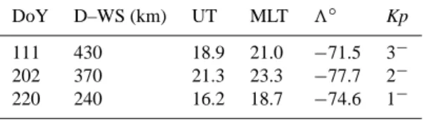
Table 3. Calculated Davis–wave source distance (D-WS), approxi-mate mid-time of wave generation (UT and MLT), magnetic latitude of source, and Kp at launch.
DoY D–WS (km) UT MLT 3◦ Kp
111 430 18.9 21.0 −71.5 3− 202 370 21.3 23.3 −77.7 2− 220 240 16.2 18.7 −74.6 1−
From the travel directions and Davis-source distances, we find the approximate source location by calculating back, in time, along the wave path, correcting for the Coriolis effect. A wave-launch time can also be found, strictly speaking, the mid-time of wave production, as time integrated prop-erties are measured. Converting the source geographic loca-tion into geomagnetic coordinates via the GEO-CGM pro-gram gives an estimate of the time of wave launch in mag-netic local time (MLT). Davis-source distances, wave launch times (in UT and magnetic local time), the calculated ge-omagnetic latitude (3) of the source, and the 3-hourly Kp index at launch are given in Table 3. Calculated source posi-tions for the waves range from 3 ∼ −71 to −78◦, and have an approximate mid-time of generation ranging from 19 to 23 hours MLT.
All-sky data taken up to ∼1 hour before the calculated wave launch times were inspected, and for DoY 111 and DoY 220 the poleward edge of the oval was well to the mag-netic north of Davis. For DoY 202 overhead aurora was seen up to 30 minutes before launch; this is the wave with a source location well to the magnetic south of Davis. On this night the 3-hourly Kp in the 18–21 UT interval was 5−. This was just prior to the estimated mid-time of launch. It seems likely that the oval was over Davis at this time, following a pole-ward sub-storm surge.
The latitude of the oval can be estimated via the Fel’dshteyn (1963) parameterisation of Holzworth and Meng (1975). For low activity, the poleward boundary is near geomagnetic lati-tude 3 = −73◦, and the equatorward border near 3 ∼ −69◦,
at midnight MLT. For moderate activity the corresponding latitudes are −72◦ and −65◦, respectively. Siscoe (1991)
notes the poleward border of the oval is much more dynamic than the equatorward border.
The waves have sources near or somewhat poleward of the poleward edge of the representative, near-midnight, au-roral oval. However, because of the uncertainties in the exact time of launch, and the rapid and large movement of the oval, we cannot determine the exact source position relative to the instantaneous oval. Attempts to address this question fur-ther, using both our ground-based AI data (as noted above) or satellite images, are subject to the uncertainty in the loca-tion of the wave source. We can conclude, however, that a source near the poleward auroral oval boundary is consistent with aspects of the results of De Deuge et al. (1994). Hall et al. (1999) also found evidence for wave sources slightly poleward of the usual (northern) auroral zone. Bristow et al.
(1994) found the sources of northern hemisphere medium-scale waves seen during daylight hours were either near lo-cal magnetic noon at 3 ∼ +80◦, or 3 ∼ +75◦and 16 hours
MLT. Interestingly, both locations are also just poleward of the low activity auroral oval at these MLTs, and the second is comparable (albeit, in the opposite hemisphere) to the cal-culated source position of the DoY 220 wave.
Magnetic local times of wave launch can be compared to when upward winds were seen over Mawson station (In-nis et al., 1997, Fig. 1, magnetic midnight at Mawson is ∼22:30 UT). Vertical winds at Mawson were seen from ∼18 hours to ∼04 hours MLT, with most occurring from ∼22 hours to ∼01 hours MLT. Upward wind events and wave generation appear to be linked to processes occurring on the poleward edge of the night-side oval, in the hours preceeding magnetic midnight. However, a direct connection between these two phenomena cannot yet be considered established.
Existence of high-latitude sources of equatorward propa-gating waves has been known for some time (see references cited earlier). It is reasonable to expect such sources can generate poleward propagating waves as well. For example, Mayr et al. (1990) interpret certain DE-2 observations by a model which includes both an equatorward and a poleward travelling wave. Modelling studies by Millward et al. (1993) and Balthazor and Moffett (1999) identify the generation of poleward- and equatorward-travelling waves in response to a high-latitude electric field enhancement. The waves detected in this work appear to be generated in or near the auroral oval, although their exact origin is not yet clear.
Only a small number of waves were seen in our data, but as noted, there is evidence for wave activity on at least three of the eleven nights when conditions were suitable for detec-tion. The waves border on the detection limit of our current FPS, and it is likely that comparable or smaller amplitude waves could be present and not be detected. MacDougall et al. (1997) noted their data indicated small vertical veloc-ity oscillations were almost always present, but the weaker oscillations, some of them probably due to lower amplitude waves, were not suitable for analysis. Hall et al. (1999) report similar findings for equatorward propagating waves. Additionally, our analysis selects only periodic oscillations. It would be important to quantify the properties of smaller amplitude oscillations, and possible non-periodic wave vari-ations, in order to obtain a more complete understanding of the polar cap wave spectrum. Establishing the nature and number of polar cap waves may be important for understand-ing the detailed dynamics and thermodynamics of the polar cap. An analysis of 5 years of 3FP data from Davis is in progress.
6 Conclusion
We have performed a detailed search for periodic variations in the vertical wind and photometric intensity time series from FPS and 3FP data from Davis station in 1999. There is evidence for a small number of oscillations consistent with
polar cap gravity waves. Assuming a wave source at the auroral electrojet height of ∼125 km, and wave ascent an-gles consistent with the properties of gravity waves, we find source locations for the waves appear to be in or near the poleward edge of the auroral oval, at magnetic local times up to 5 hours before magnetic midnight.
Acknowledgements. Dr. Vladimir Papitashvili (University of
Michi-gan) supplied the fortran program GEO-CGM and information re-garding its operation. NASA National Space Science Data Cen-ter provided software for calculating the Fel’dshteyn auroral ovals. Support for the operation of the Davis FPS is from the Australian Antarctic Division (AAD), the Antarctic Science Advisory Com-mittee, and the Australian Research Council. Ray Morris (AAD) provided useful comments on the draft manuscript. We thank Lloyd Symons and Frances Phillips for assistance with the FPS, 3FP, and AI in 1999, and the other members of the Davis 1999 Australian National Antarctic Research Expeditions for their support. John In-nis acknowledges the hospitality of the University of Alaska, Fair-banks, during part of the time this paper was in preparation. We thank the referees for a careful reading of the manuscript and help-ful comments.
Topical Editor M. Lester thanks two referees for their help in evaluating this paper.
References
Aruliah, A. L. and Rees, D., The trouble with thermospheric vertical winds: geomagnetic, seasonal and solar cycle dependence at high latitudes, J. Atmos. Terr. Phys., 57, 597–609, 1995.
Balthazor, R. L. and Moffett, R. J., Morphology of large-scale traveling atmospheric disturbances in the polar thermosphere, J. Geophys. Res., 104, 15–24, 1999.
Bristow, W. A., Greenwald, R. A., and Samson, J. C., Identification of high-latitude acoustic gravity waves sources using the Goose Bay HF radar, J. Geophys. Res., 99, 319–331, 1994.
Bristow, W. A., Greenwald, R. A., and Villain, J. P., On the sea-sonal dependence of medium-scale atmospheric gravity waves in the upper atmosphere at high latitudes, J. Geophys. Res., 101, 15685–15699, 1996.
Chandra, S., Krankowsky, D., Lammerzahl, P., and Spencer, N. W., Auroral origin of medium scale gravity waves in neutral compo-sition and temperature, J. Geophys. Res., 84, 1891–1897, 1979. Chimonas, G. and Hines, C. O., Atmospheric gravity waves
launched by auroral currents, Planet. Space Sci., 18, 565–582, 1970.
Conde, M. and Dyson, P. L., Thermospheric vertical winds above Mawson, Antarctica, J. Atmos. Terr. Phys., 57, 589–597, 1995. Crowley, G. and Williams, P. J. S., Observations of the source and
propagation of atmospheric gravity waves, Nature, 328, 231– 233, 1987.
De Deuge, M. A., Greet, P. A., and Jacka, F., Optical observations of gravity waves in the auroral zone, J. Atmos. Terr. Phys., 56, 617–629, 1994.
Fel’dshteyn, Y. I., Some problems concerning the morphology of auroras and magnetic disturbances at high latitudes, Geomagn. Aeronomy, 3, 183–192, 1963.
Francis, S. H., Global propagation of atmospheric gravity waves: A review, J. Atmos. Terr. Phys., 37, 1011–1054, 1975.
Georges, T. M., HF doppler studies of travelling ionospheric dis-trubances, J. Atmos. Terr. Phys., 30, 735–746, 1968.
J. L. Innis et al.: Thermospheric gravity waves in the southern polar cap 543
Hall, G. E., MacDougall, J. W., Cecile, J.-F., Moorcroft, D. R., and St.-Maurice, J. P., Finding gravity wave source positions using the Super Dual Auroral Radar Network, J. Geophys. Res., 104, 67–78, 1999.
Heisler, L. H., Anomalies in ionosonde records due to travelling ionospheric disturbances, Aust. J. Phys., 11, 79–90, 1958. Hernandez, G. and Roble, R. G., Observations of large-scale
ther-mospheric waves during geomagnetic storms, J. Geophys. Res., 83, 5531–5538, 1978.
Herrero, F. A., Mayr, H. G., Harris, I., Varosi, F., and Meriwether, J. W. Jr., Thermospheric gravity waves near the source: compar-ison of variations in neutral temperature and vertical velocity at Sondre Stromfjord, Geophys. Res. Lett., 1, 939–942, 1984. Hines, C. O., Propagation velocities and speeds in ionospheric
waves: A review, J. Atmos. Terr. Phys., 36, 1179–1204, 1974. Hocke, K. and Schlegel, K., A review of atmospheric gravity waves
and travelling ionospheric disturbances: 1982–1995, Ann. Geo-physicae, 14, 917–940, 1996.
Holzworth, R. H. and Meng, C.-I., Mathematical representation of the auroral oval, Geophys. Res. Lett., 2, 377–380, 1975. Hunsucker, R. D., Atmospheric gravity waves generated in the
high-latitude ionosphere: A review, Rev. Geophys. Space Res., 20, 293–315, 1982.
Innis, J. L., Greet, P. A., and Dyson, P. L., Fabry-Perot spectrometer observations of the auroral oval/polar cap boundary above Maw-son, Antarctica, J. Atmos. Terr. Phys., 58, 1973–1988, 1996. Innis, J. L., Dyson, P. L., and Greet, P. A., Further observations
of the thermospheric vertical wind at the auroral oval/polar cap boundary, J. Atmos. Sol.-Terr. Phys., 59, 2009–2022, 1997. Innis, J. L., Greet, P. A., and Dyson, P. L., Are polar cap gravity
waves a heat source for the high-latitude thermosphere?, Geo-phys. Res. Lett., 25, 1487–1490, 1998.
Innis, J. L., Greet, P. A., Murphy, D. J., Conde, M. G., and Dyson, P. L., A large vertical wind in the thermosphere at the auroral oval/polar cap boundary seen simultaneously from Mawson and Davis, Antarctica, J. Atmos. Sol.-Terr. Phys., 61, 1047–1058, 1999.
Ishii, M., Oyama, S., Nozawa, S., Fujii, R., Sagawa, E., Watari, S., and Shinagawa, H., Dynamics of the neutral wind in the po-lar region observed with two Fabry-Perot inteferometers, Earth Planets Space, 51, 833–844, 1999.
Jacka, F., Application of Fabry-Perot spectrometers for measure-ment of upper atmosphere temperatures and winds, Handbook for MAP, 13, 19–40, 1985.
Johnson, F. S., Hanson, W. B., Hodges, R. R., Coley, W. R., Carig-nan, G. R., and Spencer, N. W., Gravity waves near 300 km over the polar caps, J. Geophys. Res., 100, 23993–24002, 1995. Kanasewich, E. R., Time sequence analysis in geophysics,
Univer-sity of Alberta Press, Alberta, 1981
Lewis, R. V., Williams, P. J. S., Millward, G. H., and Quegan, S., The generation and propagation of atmospheric gravity waves from activity in the auroral electrojet, J. Atmos. Terr. Phys., 58, 807–820, 1996.
Ma, S. Y., Schlegel, K., Xu, J. S., Case studies of the propaga-tion characteristics of auroral TIDs with EISCAT CP2 data us-ing maximum entropy cross-spectral analysis, Ann. Geophysi-cae, 16, 161–167, 1998.
MacDougall, J. W., Hall, G. E., and Hayashi, K., F-region gravity waves in the central polar cap, J. Geophys. Res., 102, 14513– 14530, 1997.
Mayr, H. G., Harris, I., Herrero, F. A., Spencer, N. W., Varosi, F.,
and Pesnell, W. D., Thermospheric gravity waves: observa-tions and interpretation using the transfer function model (TEM), Space Sci. Rev., 54, 297–375, 1990.
Millward, G. H., Quegan, S., Moffet, R. J., Fuller-Rowell, T. J., and Rees, D., A modelling study of the coupled ionospheric and ther-mospheric response to an enhanced high-latitude electric field event, Planet. Space Sci., 41, 45–56, 1993.
Munro, G. H, Travelling ionospheric disturbances in the F-region, Aust. J. Phys., 11, 91–112, 1958.
Porter, H. S., Silverman, S. M., and Tuan, T. F., On the behavior of airglow under the influence of gravity waves, J. Geophys. Res., 79, 3827–3833, 1974.
Porter, H. S. and Tuan, T. F., On the behavior of the F–layer under the influence of gravity waves, J. Atmos. Terr. Phys., 36, 135– 157, 1974.
Price, G. D., Smith, R. W., and Hernandez, G., Simultaneous mea-surements of large vertical winds in the upper and lower thermo-sphere, J. Atmos. Terr. Phys., 57, 631–643, 1995.
Rees, D., Smith, R. W., Charelton, P. J., McCormac, F. G., Lloyd, N., and Steen, ˚A., The generation of vertical thermospheric winds and gravity waves at auroral latitudes–I. Observations of vertical winds, Planet Space Sci., 32, 667–684, 1984a.
Rees, D., Smith, M. F., and Gordon, R., The generation of vertical thermospheric winds and gravity waves at auroral latitudes–II. Theory and numerical modelling of vertical winds, Planet. Space Sci., 32, 685–705, 1984b.
Richmond, A. D., Gravity wave generation, propagation, and dis-sipation in the thermosphere, J. Geophys. Res., 83, 4131–4145, 1978.
Richmond, A. D. and Roble, R. G., Dynamic effects of aurora-generated gravity waves on the mid-latitude ionosphere, J. At-mos. Terr. Phys., 41, 841–852, 1979.
Siscoe, G. L., What determines the size of the auroral oval?, Auroral Physics, 159–175, eds. C.-I. Meng, M.J. Rycroft, and L.A. Frank, Cambridge University Press, 1991.
Smith, R. W., Vertical winds: a tutorial, J. Atmos. Sol.-Terr. Phys., 60, 1425–1434, 1998.
Smith, R. W. and Hernandez, G., Vertical winds in the thermosphere within the polar cap, J. Atmos. Terr. Phys., 57, 611–620, 1995. Spencer, N. W., Theis, R. F., Wharton, L. E., and Carignan, G. R.,
Local vertical motions and kinetic temperatures from AE–C as evidence for aurora induced gravity waves, Geophys. Res. Lett., 3, 313–316, 1976.
Spencer, N. W., Wharton, L. E., Carignan, G. R., and Maurer, J. C., Thermospheric zonal winds, vertical motions and temperatures as measured from Dynamics Explorer, Geophys. Res. Lett., 9, 953–956, 1982.
Testud, J. and Vasseur, G., Ondes de gravit´e dans la thermosph`ere, Ann. G´eophys., 25, 525–546, 1969.
Williams, P. J. S., Crowley, G., Schlegel, K., Virdi, T. S., McCrea, I., Watkins, G., Wade, N., Hargreaves, J. K., Lachlan-Cope, T., Muller, H., Baldwin, J. E., Warner, P., van Eyken, A. P., Hap-good, M. A., and Rodger, A. S., The generation and propagation of atmospheric gravity waves observed during the Worldwide At-mospheric Gravity-wave Study (WAGS), J. Atmos. Terr. Phys., 50, 323–338, 1988.
Williams, P. J. S., Virdi, T. S., Lewis, R. V., Lester, M., Rodger, A. S., McCrea, I. W., and Freeman, K. S. C., Worldwide atmo-spheric gravity-wave study in the European sector, 1985–1990, J. Atmos. Terr. Phys., 55, 683–696, 1993.