HAL Id: hal-00295734
https://hal.archives-ouvertes.fr/hal-00295734
Submitted on 8 Sep 2005
HAL is a multi-disciplinary open access
archive for the deposit and dissemination of
sci-entific research documents, whether they are
pub-lished or not. The documents may come from
teaching and research institutions in France or
abroad, or from public or private research centers.
L’archive ouverte pluridisciplinaire HAL, est
destinée au dépôt et à la diffusion de documents
scientifiques de niveau recherche, publiés ou non,
émanant des établissements d’enseignement et de
recherche français ou étrangers, des laboratoires
publics ou privés.
CLABAUTAIR: a new algorithm for retrieving
three-dimensional cloud structure from airborne
microphysical measurements
R. Scheirer, S. Schmidt
To cite this version:
R. Scheirer, S. Schmidt. CLABAUTAIR: a new algorithm for retrieving three-dimensional cloud
structure from airborne microphysical measurements. Atmospheric Chemistry and Physics, European
Geosciences Union, 2005, 5 (9), pp.2333-2340. �hal-00295734�
SRef-ID: 1680-7324/acp/2005-5-2333 European Geosciences Union
Chemistry
and Physics
CLABAUTAIR: a new algorithm for retrieving three-dimensional
cloud structure from airborne microphysical measurements
R. Scheirer1and S. Schmidt2
1Institut f¨ur Physik der Atmosph¨are, DLR, Oberpfaffenhofen, Germany 2Leibniz-Institute for Tropospheric Research, Leipzig, Germany
Received: 20 October 2004 – Published in Atmos. Chem. Phys. Discuss.: 23 December 2004 Revised: 8 June 2005 – Accepted: 24 August 2005 – Published: 8 September 2005
Abstract. A new algorithm is presented to reproduce the
three-dimensional structure of clouds from airborne mea-surements of microphysical parameters. Data from individ-ual flight legs are scanned for characteristic patterns, and the autocorrelation functions for several directions are used to extrapolate the observations along the flight path to a full three-dimensional distribution of the cloud field. Thereby, the mean measured profiles of microphysical parameters are imposed to the cloud field by mapping the measured prob-ability density functions onto the model layers. The algo-rithm was tested by simulating flight legs through synthetic clouds (by means of Large Eddy Simulations (LES)) and ap-plied to a stratocumulus cloud case measured during the first field experiment of the EC project INSPECTRO (INfluence of clouds on the SPECtral actinic flux in the lower TROpo-sphere) in East Anglia, UK. The number and position of the flight tracks determine the quality of the retrieved cloud field. If they provide a representative sample of the entire field, the derived pattern closely resembles the statistical properties of the real cloud field.
1 Introduction
According to IPCC (2001), the parameterization of the cloud-radiation interaction is one of the largest sources of uncertainty in our prediction of future climate. To improve such parameterizations, detailed three-dimensional (3-D) ra-diative transfer studies are required, to quantify the impact of cloud inhomogeneity on the radiation budget.
A challenge in three-dimensional (3-D) radiative transfer is the generation of realistic clouds as input for sophisticated radiative transfer models (e.g. Borde and Isaka, 1996; Petty, 2002). Currently, it is not possible to derive the required
Correspondence to: R. Scheirer
distribution of liquid water content and droplet sizes from observations of a single instrument. Radar and lidar instru-ments (or even better combinations of both) are excellent in retrieving 1-D profiles or cross sections if they have scan-ning facilities. For the retrieval of 3-D structures (if there is no special 3-D scanning facility) they are reliant on hor-izontal wind and a horhor-izontal isotropic cloud field (Evans and Wiscombe, 2004). Passive satellite remote sensing in-struments may provide a detailed horizontal distribution but fail to give reliable information about vertical profiles (e.g. Crewell et al., 1999). In-situ observations, on the other hand, may give data for any location but are usually restricted to only a few point measurements, e.g. along an aircraft flight track. Physical cloud-models (e.g. LES) can provide the full 3-D information of all needed microphysical properties in a realistic manner (Stevens and Lenschow, 2001) but much ef-fort is needed to make them reproduce the properties of mea-sured cloud fields.
Clouds vary significantly in the three spatial dimensions and in time. Common airborne instruments sample volumes in the magnitude of a few liters during a single leg while cu-mulus clouds, for example, often cover a volume of around 109m3. The major part of the clouds are thus not consid-ered for its characterization which is a significant limitation because of the cloud’s large variability (Evans et al., 2003). Therefore, aircraft measurements alone seem to be gener-ally not sufficient to characterize the properties of inhomo-geneous cloud layers.
On the other hand, the heterogeneous structure of cloud fields is often characterized by strong vertical and horizontal correlations (with correlation lengths depending for example on turbulent cell-size or topography), allowing to general-ize “needle in a haystack”, that is very sparse, but inline (i.e. taken during flight legs on a more or less straight line) aircraft measurements for the whole cloud. This structure is orga-nized by entrainment and turbulence at a spectrum of length scales. For micro-scale turbulence this is shown by Shaw et
2334 R. Scheirer and S. Schmidt: Retrieving cloud structure from airborne measurements
X
Y
Y
X
Y
X
Y
X
d)
b)
c)
a)
?
Fig. 1. The four main steps of CLABAUTAIR. This figure illustrates an approach to retrieve 3-D clouds from aircraft measurements.
al. (1998). The basic assumption behind the algorithm pre-sented here is that the atmospheric conditions determining the turbulent spectrum do not change markedly within the model domain. For homogeneous conditions within a limited area and time period, a similar behavior of the corresponding cloud field is expected. Thus, in some cases such as for strat-iform overcast or broken cloud fields, aircraft line measure-ments along a limited number of flight legs are representative for the whole layer under stable conditions. For example, Los and Duynkerke (2000) and R¨ais¨anen et al. (2003) gen-erated two-dimensional cloud fields from in-cloud aircraft measurements. However, they required some assumptions about cloud top and base structure, and about the profile of microphysical parameters.
This study introduces a new algorithm which generates 3-D cloud fields representing the statistical properties of a measured cloud field by using in situ data of liquid water con-tent and effective radius. In Sect. 2, the extrapolation of the 3-D structure from one-dimensional aircraft measurements, and thus the filling of the gaps is described. Subsequently, the algorithm is applied to a synthetic cloud field (Sect. 3) and to a measured cloud case (Sect. 4), and a preliminary discussion of its applicability is given.
2 Algorithm
An automated algorithm (cloud liquid water content and ef-fective radius retrieval by an automated use of aircraft
mea-surements (CLABAUTAIR)) has been developed with the in-tention to generate a 3-D cloud field which reproduces the statistical properties of the microphysical aircraft measure-ments. The measurements of liquid water content (LWC) and effective radius (Reff) are scanned, and the probability density functions PDFs as well as the autocorrelation func-tions are determined for every layer, defined by the user. The patterns which are found in the autocorrelation functions are then used to extrapolate the aircraft data to a complete 3-D field.
This method is illustrated in Figs. 1a–d. Starting with mea-surements in a single horizontal layer the main directions sampled by the aircraft are identified. This means, the data-points are sampled by relative angular bins (e.g. directions from one point to each other point) layer by layer, to spot long straight lines of measurements (Fig. 1a). This is neces-sary to avoid aliasing due to the connection of different flight legs and thus to correlate only data collected within a time interval during which the cloud can be considered constant. Next, the autocorrelation functions along these directions are calculated (Fig. 1b). As far as the cloud movement is slow compared to the aircraft’s speed and cloud structure is stable, advection should not be a problem since the autocorrelation is not seriously affected.
Then the measured LWC and Reff are replaced by their anomalies (i.e. deviations from the layers mean) and used for the initial field. Since it is a ground-fixed (Eulerian) co-ordinate system, the measurements have to be shifted with the cloud movement vector which may differ from the wind
vector (e.g. for orographic clouds). To extrapolate the obser-vations, individual empty boxes are randomly selected within the 3-D space. The requested parameters ξ (anomaly of LWC or Reff) for each of these boxes are calculated by a weighted average over the I filled boxes along the J main directions (Fig. 1c). Horizontal anisotropies are taken into account by assigning each autocorrelation function to a specific direc-tion. The weighting is performed by the autocorrelation co-efficient r valid for the distance δ=|x−xi,j|between the
cen-ter of the current (already filled) box at (xi,j) and the ith box
under calculation for the j th direction at (x) (marked with a question mark in Fig. 1c):
ξ(x) = J P j =1 I (j ) P i=1 rj(|x − xi,j|)ξ(xi,j) J P j =1 I (j ) P i=1 rj(|x − xi,j|) . (1)
If the weighting sum
J X j =1 I (j ) X i=1 rj(|x − xi,j|) (2)
fails to reach a certain threshold, calculation of ξ(x) will be postponed. Initially1this threshold is set to 3 to take into ac-count only calculations with a minimum attendance of con-tributing boxes. Due to the use of anomalies instead of abso-lute values this approach is also meaningful in case of neg-ative autocorrelation coefficients. Adjacent boxes from the next layer above and below the chosen one (if already cal-culated) are taken into account with a fixed weight2of 0.95. This step is repeated until all boxes are filled. Finally, the PDF of the measurements (including the cloud-free parts to permit cloud fractions smaller than 1) are mapped onto the thus derived spatial distributions. This mapping is done for all cloudy layers separately by first calculating the cloud frac-tion cf from measurements. Then setting (1−cf)Ntot(Ntotis the total box number per layer) boxes with the lowest value of the anomalies to zero. For the remaining boxes, a modified random number generator that reproduces any given distribu-tion (in this case the requested PDFs) is used. The genera-tor is started cf Ntot times and finally the values reproduced this way are assigned to the remaining boxes according to the sorting order (the largest reproduced value to the box with the largest anomaly-value, the second largest reproduced value to the second largest anomaly, and so on). Figure 1d shows 1If this threshold results in accepting less than 1% of the
calcu-lations it will be reduced temporarily.
2Actually this weight depends on the vertical resolution but for
magnitudes used in this study, the stated weight is reasonable. In the moment we are collecting profiles of LWC and Reffto calculate
res-olution dependent vertical correlation coefficients to base our pre-sumptions on facts, but anyway the vertical correlation coefficient can not be measured for any individual case hence it must be pa-rameterized.
the final cloud field. This last step ensures to keep the re-produced cloud field close to the measurements. At the same time it roughens the field that was smoothed by averaging previously. In a further consequence the structure or spa-tial pattern of this field is only determined by the sorting se-quence resulting from the weighted averaging, performed by Eq. (1).
The possible spatial resolution depends on the number, the direction, and the length of the flight legs, the sampling rate, and on the autocorrelation function. For the cases used in this study, horizontal resolutions between 40 m and 250 m and vertical resolutions between 20 m and 100 m were used.
3 Test of the method
The algorithm was tested with a synthetic cloud field. A large eddy simulation (LES) of a stratocumulus field pro-vided by the Intercomparison of 3-D Radiation Codes (I3RC, at http://i3rc.gsfc.nasa.gov) was chosen for this test. The LES cloud field has a horizontal resolution of 55 m and a vertical resolution of 25 m. With 64 times 64 boxes the do-main size is 3.5×3.5 km2. The clouds are located between 400 m and 800 m altitude. Within this cloud field samples were taken by virtual flights. Each single flight (out of 200 in total) starts at the center of the area at the ground with a random direction and an ascent angel of 10◦. A new direc-tion is selected by random if the border is reached. If cloud top is exceeded, the descent starts in the same manner but at a flatter angle (0.5◦). Samples are taken every 10 m with a random error of ±5% added to the data. A cloud retrieval is based on about 10 to 20 flight-legs (depending on random directions). The distance covered by the aircraft within the cloudy layers is constant. For the ascent we got (climbing height 400 m, 10◦ascending angle) about 2304 m and for the
descent (0.5◦ descending angle) about 45 837 m. In result
typically about 2% of the total model boxes are described by virtual measurements so that about 98% had to be calculated by our algorithm.
For the retrieved cloud field, the horizontal resolution was set to 43 m and the vertical to 39 m to avoid the unrealistic case of model boxes that fit perfectly to the source cloud. Three examples of different flight patterns and the result-ing retrievals are given in Fig. 2. We found that the gain in information by following the same flight track at differ-ent altitudes is marginal (left column) because of the large vertical correlation of microphysical properties. Therefore we recommend random-like flight patterns (middle and right column) to get more independent information and to sample a larger area.
A comparison of original and reproduced power-spectra is shown in Fig. 3 These spectra were averaged over three hor-izontal tracks in E-W direction with about 1.5 km N-S sepa-ration. The different colors represent the three different real-izations of the original cloud as shown in Fig. 2. The power
2336 R. Scheirer and S. Schmidt: Retrieving cloud structure from airborne measurements
Fig. 2. Three examples of different flight patterns within a LES cloud field (upper row, 3.5×3.5 km2). Red arrows mark ascending and blue arrows descending legs. Considered are only flight legs meeting the cloudy altitudes (400 m–800 m). The retrieved cloud structures are given in the lower row (3.526×3.526 km2). The plotted parameter is the liquid water path in arbitrary units just to give an impression of the cloud structures. 1 10 1 10 100 1000 LES version 0 version 1 version 2 Pn n [1/km]
Fig. 3. Comparison of original (black) and reconstructed (colored) power-spectra. Different colors distinguish between different real-izations. All spectra are averages over 3 horizontal legs.
spectrum from the original LES cloud (black line) shows a step at a wavenumber of 6 km−1which cannot be seen in the reproduced power spectra. This step is most likely the re-sult of LES internal low-pass filtering. Due to crossing the boxes in different than right angles more variability is found on smaller scales. Therefore, the reproduced field does not exhibit this break in the power spectrum.
0 10 20 30 Optical Thickness 0.00 0.02 0.04 0.06 0.08 0.10 Rel. Frequency Original Cloud Retrieval (Triangle Flight) Retrieval Mean (200 Random Flights) 68% Confidence Interval
Fig. 4. Frequency of optical thicknesses for the original cloud field (green), the retrieval from triangular flight (red), and the mean of 200 retrievals (blue). The shaded area marks the 68% confidence interval.
Figure 4 shows the frequency of optical thicknesses for the original cloud field as well as for the mean of 200 retrievals based on random flights. The original cloud fraction is 0.926 while the retrieval-mean gives 0.959 with a standard devia-tion of 0.018. This overestimadevia-tion of cloud-fracdevia-tion could
Fig. 5. Two-dimensional PDF of the measured liquid water content and the effective drop radius at three altitudes to illustrate the vertical distribution of horizontal data spread.
be a hint that the assumed vertical correlation coefficient of 0.95 is too small for the given vertical resolution, because the minimum in cloud fraction is realized with a maximum overlap. Any deviation from this maximum overlap towards a random or even minimum overlap increases the cloud frac-tion. Therefore the vertical correlation coefficient that de-termines the overlap could be responsible for this bias. The under-representations of extreme optical thicknesses in Fig. 4 by simulated cloud fields may also vanish if a larger vertical correlation coefficient would be applied. Columns with very large and very small τ should grow at the expense of columns with medium τ . The complete distribution should be shifted towards the original one.
For the cloud volume the retrieval provides a mean of 1.860 km3and a standard deviation of 0.123 km3 while the original volume is 1.874 km3. So we found CLABAUTAIR to reproduce the cloud fields features in a reasonable accu-racy.
4 Application to field measurements
4.1 Aircraft data
The first application of the algorithm to in-situ microphysical data was performed for a cloud situation which was measured during the first field experiment of the EC project INSPEC-TRO (influence of clouds on the spectral actinic flux in the lower troposphere) on 14 September 2002, on the coast of East Anglia, United Kingdom. On this day, a stable stra-tus layer which was moving into land at a speed of about 10 m/sec was observed between 500 and 1100 m altitude. The microphysical measurements used for this study were performed with a two-propeller research aircraft, a Parte-navia P68B, which was equipped with meteorological, mi-crophysical, and radiation instrumentation. The microphys-ical cloud properties were measured with a Fast Forward Scattering Spectrometer Probe (Fast-FSSP, Brenguier et al.,
1998) and a Particle Volume Monitor (PVM-100, Gerber et al., 1994). The Fast-FSSP measures the cloud drop size dis-tribution by detecting the forward scattering signal of each individual droplet passing a laser beam. From the drop size distribution, bulk parameters such as the LWC, the drop con-centration, and Reffcan be derived (Schmidt, 2004). In con-trast, the PVM-100A measures the LWC directly by detect-ing the scatterdetect-ing signal of an ensemble of droplets. For this study, the LWC measurements by the PVM-100A were used because of the high accuracy and temporal resolution of the data. The effective droplet radius Reff was derived from the FSSP measurements because of its higher accuracy for this parameter.
In order to examine the three-dimensional cloud structure, several ascents and descents through the cloud layer were flown by the aircraft. In addition, one triangular flight pat-tern within the layer was performed. Figure 5 shows the two-dimensional PDFs of the LWC and Reff for three dif-ferent altitudes. They were determined by combining the measurements of the PVM-100A and the Fast-FSSP, and bin-ning them into several height layers. The color scale in the plots corresponds to the probability of a particular LWC and
Reff at the respective level. These two-dimensional PDFs
reflect the microphysical properties accumulated throughout the cloud layer. The layer cloud fraction as a macrophysical property is also deduced from the microphysical measure-ments. The horizontal structure is contained in the autocor-relation functions which are calculated for the three legs of the triangle.
4.2 Retrieved cloud fields
For the INSPECTRO cloud case which is described in Sect. 4.1, the output of the algorithm was quantitatively com-pared with the measurements by analyzing the measured and retrieved profiles of the LWC and the power spectra along horizontal lines.
2338 R. Scheirer and S. Schmidt: Retrieving cloud structure from airborne measurements
−3
Fig. 6. Measured and reconstructed LWC profile. Note that the range of measurements does not fit exactly to the range of recon-structed LWCs. See text for details.
In Fig. 6, measured and reconstructed profiles of the LWC are displayed. The circles show the PVM-100A measure-ments. The cloud top and base heights vary approximately within 200 m. At 800 m, the horizontal flight pattern was per-formed. The range of LWC values measured at this altitude reflects the high variability which prevails even in a stratus layer. The solid blue line shows the mean reconstructed LWC profile. The error bars indicate the standard deviation which was found throughout the grid. It reproduces well the range of LWC values which were measured during the horizontal leg. The dashed and dash-dotted blue lines correspond to the minimum and maximum LWC values, respectively, which are generated at the levels. One may expect that due to the approach described in Sect. 2 the range of reproduced LWC should exactly fit to the range of measurements. Deviations in the maximum are mainly induced by the resolution of the stored PDF or by dominating measurements3with no liquid water found (which are not shown in Fig. 6). The underes-timation of the reproduced minimum can also be explained by a consideration of zero-values. In general, the determi-nation of the reproduced cloud field to the measured span of microphysical properties should only become a problem if the measurements are not representative. Though it is rather unlikely to measure exactly the minimum and maximum of LWC and Reff within the present domain, even so one may expect to get a quantitative overview in the sense that the 3Since we used a random number generator able to reproduce
any given distribution function (see Sect. 2), the reproduced values may not fill the whole range of the original measurements if there is a dominating part in this range. Figure 6 for example provides many zero values in altitudes between 1000 m and 1100 m. Therefore only a few boxes in this layer need an assigned LWC and Reff. That is why the population could be found too small to cover the whole measured range. 0.1 1 1E-5 1E-4 1E-3 0.01 0.1 1 Power Spectra
measured along track reconstructed along track across track n -5/3 P n [(g/m 3 /(1/km)) 2 /(1/km)] n [1/km]
Fig. 7. Power Spectra calculated from in situ aircraft measurements (black dotted) of the LWC and its reconstruction (colored). Also shown is the k−5/3scaling law (thin solid line).
dominant modes and the general shape of the real distribu-tion are met by the measurements. Deviadistribu-tions are unlikely to alter the reproduced cloud substantially. Since one can never rule out the possibility to have the extrema included in the measured data, an extension of the range of values in the re-produced cloud beyond the actually measured range does not seem to be justified.
The horizontal structure of the measured and reconstructed cloud is compared in Fig. 7 by means of power spectra P (k) where k denotes the wavenumber. The dotted line with open circles shows the power spectrum which was calculated from PVM-100A measurements along one of the legs of the tri-angular pattern within the cloud layer (about 27 km length). The measurements are in agreement with the k−5/3scaling law (thin solid line) which is typically found for real clouds (Davis et al., 1996). The power spectra from the reproduced cloud were obtained by calculating power spectra over hori-zontal lines throughout the grid and by subsequent averaging. The direction of the lines was chosen along and across the flight leg whose power spectrum is displayed. The red line shows the averaged power spectrum of lines parallel to the leg direction. In general the k−5/3scaling is well reproduced. The blue line shows the averaged power spectrum from lines across the leg direction. In this case, the characteristic of this curve shows a better agreement to the measurements. The power spectra for the PVM-100A data measured along other legs of the in-cloud pattern are similar to the power spectrum which is displayed in Fig. 7. Thus, the differences between power spectra along different directions of the reproduced cloud field cannot be explained by the measurements. How-ever, the power spectra of the reproduced cloud field agree with the observations within the range of measurement un-certainty.
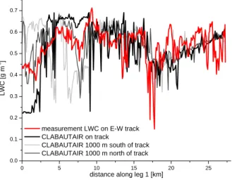
Finally Fig. 8 gives an impression of the structure and the variability of an in situ LWC measurement series. The red
0 5 10 15 20 25 0.0 0.1 0.2 0.3 0.4 0.5 0.6 0.7
measurement LWC on E-W track CLABAUTAIR on track
CLABAUTAIR 1000 m south of track CLABAUTAIR 1000 m north of track
LWC [g m
-3]
distance along leg 1 [km]
Fig. 8. Measured and reconstructed LWC series along an approxi-mately 27 km flight leg.
line shows the measurements along a horizontal leg – the black and gray lines show reproductions. The thick black line is directly on the flight track whereas the thinner gray lines are 1000 m off the original track.
5 Conclusions
A new algorithm for the retrieval of statistical properties of 3-D cloud fields based on aircraft measurements has been developed.
Testing our algorithm with a complete LES cloud field, we found a promising agreement between the original and retrieved cloud features. The retrieval mean cloud-fraction provides an error of about 3.6% and the retrieval mean cloud-volume an error of about 0.8%. For the sampling of cloud fields we recommend to follow random-like instead of flight patterns that imply similar paths at different altitudes.
From an application to real measurements we learned that within the measurement uncertainty, the characteristics of the simulated clouds agree with the observed counterparts.
It must be stated that the presented algorithm is limited to a moderate wind-speed and stable conditions, i.e. no signifi-cant change in the cloud pattern should occur during the mea-surements (no rapid convective growth). In our algorithm the overlap statistics is determined by the vertical correlation co-efficient. We found some hints that the presumed value of 0.95 could be too small and probably depending on the ver-tical resolution.
Rather than reproducing the original cloud situation, CLABAUTAIR supplies a cloud field whose statistical prop-erties match the aircraft measurements. This could also be valid for the spiky behavior (the intermittency, e.g. Davis et al., 1994) of natural clouds, if found within the measure-ments, i.e. if the database is really representative. Due to a general decrease of the autocorrelation function with
dis-tance, the uncertainty of the estimation increases with the distance to the measurements. We recommend to chose evenly distributed flight legs with several (random-like) ori-entations to sample as much independent information as pos-sible and to avoid unrealistic smoothing. Nevertheless, addi-tional work will be done on validation and improvement of the presented algorithm. Advanced tests (including radiative transfer tests) and comparisons with different approaches in retrieving cloud properties are in preparation.
Acknowledgements. This work was funded by the European project INSPECTRO (Influence of clouds on the spectral actinic flux in the lower troposphere), contract EVK2-2001-00135. Enviscope GmbH, Frankfurt, Germany, operated the aircraft during the experiment: Thanks to R. Maser, D. Schell, and H. Franke, and to the pilot B. Schumacher. L. Hinkelman, Langley Research Center, Hampton, USA, provided us with LES cloud fields used for preliminary tests.
Edited by: W. Conant
References
Borde, R. and Isaka, H.: Radiative transfer in multifractal clouds, J. Geophys. Res., 101(D23), 29 461–29 478, 1996.
Brenguier, J. L., Bourrianne, T., Coelho, A., Isbert, J., Peytavi, R., Trevarin, D., and Wechsler, P.: Improvements of droplet size distribution measurements with the Fast-FSSP (Forward Scatter-ing Spectrometer Probe), J. Atmos. Oceanic Technol., 15, 1077– 1090, 1998.
Crewell, S., Hasse, G., L¨ohnert, U., Mebold, H., and Simmer, C.: A Ground Based Multi-Sensor System for the Remote Sensing of Clouds, Phys. Chem. Earth (B), 24, 207–211, 1999.
Davis, A., Marshak, A., Wiscombe, W., and Cahalan, R.: Multifrac-tal characterizations of nonstationarity and intermittency in geo-physical fields: Observed, retrieved, or simulated, J. Geophys. Res., 99(D4), 8055–8072, 1994.
Davis, A., Marshak, A., Wiscombe, W., and Cahalan, R.: Scale In-variance of Liquid Water Distributions in Marine Stratocumulus. Part I: Spectral Properties and Stationarity Issues, J. Atmos. Sci., 53, 1538–1558, 1996.
Evans, K. F., Lawson, R. P., Zmarzly, P., O’Connor, D., and Wis-combe, W. J.: In situ cloud sensing with multiple scattering li-dar: Simulations and demonstration, J. Atmos. Ocean Tech., 20, 1505–1522, 2003.
Evans, K. F. and Wiscombe, W. J.: An algorithm for generating stochastic cloud fields from radar profile statistics, Atmos. Res., 72, 263–289, doi:10.1016/j.atmosres.2004.03.016, 2004. Gerber, H., Ahrends, B. G., and Ackerman, A. S.: New
micro-physics sensor for aircraft use, Atmos. Res., 31,, 235–252, 1994. IPCC: Climate change 2001: The scientific basis. Third assess-ment of the Intergovernassess-mental Panel on Climate Change (IPCC), edited by: Houghton, J. T., Ding, Y., Griggs, D. J., Noguer, M., van der Linden, P. J., Dai, X., Maskell, K., and Johnson, C. A., Cambridge Univ. Press, New York, USA, 2001.
Los, A. and Duynkerke, P. G.: Microphysical and radiative proper-ties of inhomogeneous stratocumulus: Observations and model simulations, Quart. J. R. Meteorol. Soc., 126, 3287–3307, 2000.
2340 R. Scheirer and S. Schmidt: Retrieving cloud structure from airborne measurements Pawlowska, H., Brenguier, J. L., and Salut, G.: Optimal Nonlinear
Estimation for cloud Particle Measurements, J. Atmos. Ocean Tech., 14, 88–104, 1997.
Petty, G. W.: Area-Average Solar Radiative Transfer in Three-Dimensionally Inhomogeneous Clouds: The Independently Scat-tering Cloudlet Model, J. Atmos. Sci., 59, 2910–2929, 2002. R¨ais¨anen, P., Isaac, G. A., Barker, H. W., and Gultepe, I.: Solar
ra-diative transfer for stratiform clouds with horizontal variations in liquid-water path and droplet effective radius, Quart. J. R. Mete-orol. Soc., 129, 2135–2149, 2003.
Schmidt, S.: Influence of Cloud Inhomogeneities on Solar Spec-tral Radiation, Ph.D. thesis, 105 pp., Univ. Leipzig, Germany, Leipzig, 9. July 2004.
Shaw, R. A., Reade, W. C., Collins, L. R., and Verlinde, J.: Prefer-ential concentration of cloud droplets by turbulence: Effects on the early evolution of cumulus cloud droplet spectra, J. Atmos. Sci., 55, 1965–1976, 1998.
Stevens, B. and Lenschow, D. H.: Observations, experiments and large eddy simulation, Bull. Amer. Meteor. Soc., 82, 283–294, 2001.