ORIGINAL PAPER
Overestimates of maternity and population growth rates
in multi-annual breeders
Guillaume Chapron&Robert Wielgus&
Amaury Lambert
Received: 10 February 2012 / Revised: 8 August 2012 / Accepted: 27 September 2012 / Published online: 11 October 2012 # Springer-Verlag Berlin Heidelberg 2012
Abstract There has been limited attention to estimating maternity rate because it appears to be relatively simple. However, when used for multi-annual breeder species, such as the largest carnivores, the most common estimators intro-duce an upward bias by excluding unproductive females. Using a simulated dataset based on published data, we com-pare the accuracy of maternity estimates derived from stan-dard methods against estimates derived from an alternative
method. We show that standard methods overestimate mater-nity rates in the presence of unsuccessful pregnancies. Importantly, population growth rates derived from a matrix model parameterized with the biased estimates may indicate increasing populations although the populations are stable or even declining. We recommend the abandonment of the bi-ased standard methods and to instead use the unbibi-ased alter-native method for population projections and assessments of population viability.
Keywords Maternity rate . Bias . Grizzly bear . Ursus arctos . Growth rate
Introduction
Improving management recommendations from population models is dependent upon parameterizing them with all available information in an unbiased way. For simple matrix and stage-structured population models, at least two kinds of demographic parameters are needed: survival and maternity rates. Estimating survival has been the focus of extensive research and can be done following well-established meth-ods (Thomson et al.2008; Williams et al.2002). Estimating maternity rate appears to be simpler and does not require a careful attention because accurate and unbiased estimates of maternity rate Mx (i.e., the average number of offspring this year for each of the mothers this year) are relatively easily obtained for annual breeders: one simply censuses the num-ber of offspring (No) and females (Nf), and the resulting ratio (No/Nf) provides the maternity rate for that year (Akçakaya et al. 1999). This method is, however, inade-quate for multi-annual breeders with extended birth intervals such as the largest carnivores. Three methods that were described in the study of McLellan (1989) for grizzly bears (Ursus arctos horribilis) are generally used. In Method 1
Communicated by M. Artois
Electronic supplementary material The online version of this article (doi:10.1007/s10344-012-0671-x) contains supplementary material, which is available to authorized users.
G. Chapron (*)
Grimsö Wildlife Research Station, Department of Ecology, Swedish University of Agricultural Sciences,
73091 Riddarhyttan, Sweden
e-mail: [email protected] G. Chapron
Conservation Biology Division, Institute of Ecology and Evolution, University of Bern,
Baltzerstrasse 6,
CH–3012 Bern, Switzerland R. Wielgus
Département Ecologie et Gestion de la Biodiversité, Museum National d’Histoire Naturelle,
57 rue Cuvier,
75231 Paris Cedex 05, France R. Wielgus
Large Carnivore Conservation Laboratory, Department of Natural Resource Sciences, Washington State University,
Pullman, WA 99164-6410, USA A. Lambert
Laboratoire de Probabilités et Modèles Aléatoires, UPMC Université Paris,
06, Case courrier 188, 4, Place Jussieu, 75252 Paris Cedex 05, France
(M1), reproductive rate equalled to “the total number of cubs observed divided by the total number of bear years required to produce them”. In Method 2 (M2), the repro-ductive rate equalled to “the average of each individual’s rate”. In Method 3 (M3), the reproductive rate equalled to the “average litter size divided by the average interbirth interval”. The author added that M1 and M2 included “in-formation only from female bears that were radio-tracked through at least one interbirth interval”, and on the contrary, more information was available for estimating the reproduc-tive rate using M3 because “all litter size data could be used”. An improvement of M3 appeared later in the study of Eberhardt et al. (1994) and Hovey and McLellan (1996) who developed bootstrapped estimates for Mx and associated 95 % confidence intervals for grizzly bears, using mean litter size divided by mean birth interval ratio with individual litters and birth intervals as sample units. Nevertheless, the original M3 remains the most widely used and standard method to estimate reproductive rate not only for grizzly bears but also for other large carnivores such as leopards, mountain lions, or tigers (Boyce et al.2001; Eberhardt et al.1994; Karanth and Stith1999; Logan and Sweanor2001; Mace and Waller1998; McLellan1989; McLoughlin et al.2003a; Miller1997; Pease and Mattson 1999; Schwartz et al. 2003; Wakkinen and Kasworm2004; Wielgus 2002; Wielgus and Bunnell 1994,
2000; Wielgus et al. 1994; Kerley et al.2003; Owen et al.
2010).
The problem with using these three methods is the potential for biasing estimates of Mx upwards, hence overestimating population growth and viability. It can be intuitively under-stood that no observation of newborns (afterwards termed “litter sizes of zero”) will not readily be included in calculating mean litter size. It can be equally understood that birth inter-vals (e.g., number of years between successive, successful births) must be closed to calculate mean birth interval, i.e., each individual needs at least two reproductive events to have a complete interval. Hence, litter sizes of zero and indetermi-nate or open-ended birth intervals are excluded in methods M1, M2, and M3. This potential bias could be particularly severe in unproductive populations where females commonly fail to produce a litter or have birth intervals longer than the period of study. These unproductive animals would be exclud-ed, yielding an upwardly biased estimate of Mx. Hovey and McLellan (1996) recognized this problem of a potential bias but believed it was unimportant in their grizzly bear study because only four of 14 females with observed litters failed to provide a closed interval. However, it should be mentioned that only 60 % (14 of 23) adult females were observed to produce litters in their study.
Further studies have tried to address the bias potentially introduced using methods M1, M2, and M3. Some researchers (Lambert et al. 2006) modified the standard mean litter size/mean birth interval ratio by estimating
percentage of unproductive females (those with litters of zero and indeterminate birth intervals) and multiplying the reciprocal of this percentage by the standard ratio estimate. Others (Chapron et al. 2003; McLoughlin et al. 2003b; Wielgus et al. 2001) estimated Mx using a probabilistic approach—which incorporates the probabilities of produc-ing from 0 to N offsprproduc-ing on an annual basis. Schwartz and White (2008) recognized the bias of McLellan (1989) methods and proposed a completely different approach through computing transition probabilities between female states defined as female alone, with cubs, yearlings, or 2-year olds. Garshelis et al. (2005) mentioned the potential bias in the standard method (only 13 birth intervals were closed compared to 23 open-ended intervals in their study), and they calculated Mx by proposing an alternative method (labeled M4) which is to divide each year the number of offspring by the number of females and then to compute the arithmetic mean over years. They found that their estimate of grizzly bear Mx was also among the lowest ever recorded and attributed that to some combina-tion of real biological differences and/or biased overesti-mates in other studies.
If these four different methods used to parameterize population models do not give the same results, then some conservation assessments and management strate-gies may be hazardous while appearing safe if Mx is biased upwards. Are some populations of multi-annual breeders previously estimated to be growing using the standard method M3 actually declining? Is the alterna-tive method M4 always accurate? How large is the bias in the standard method M3 and should all analyses and recommendations based on that method be reassessed using the alternative method M4? In this paper, we compare McLellan (1989) M1, M2, and mostly M3 computations of reproductive rates for multi-annual breeders against the alter-native method M4 to estimate maternity rate Mx using simu-lated data and taking the grizzly bear as an illustrative example. We compare the outcomes of each method and how they are affected by sampling duration (years of moni-toring), sample size (number of females), and population parameters. We also compare how method M3 of estimating Mx affects modeled population growth rates and provide a theoretical quantification of the bias introduced by method M3.
Methods
Illustrative example
We first consider an illustrative example based on a representative grizzly bear dataset (Table 1) to allow one to understand how methods M1, M2, M3, and M4
differ. Based on the second author knowledge of bear biology, we generate a dataset with 12 adult females studied over 6 years (a typical graduate student or agency project on large carnivores). Females in this example give birth to one to four cubs every 2–4 years, as is the accepted norm for most grizzly bear popula-tions (Schwartz et al. 2003). Environmental stochasticity is built into the dataset with good and bad years (e.g., year 10good, year 60bad) to reflect typical booms and busts centered on bear foods such as berry crops, salm-on, and ungulate prey (Wielgus 2002).
With method M1, one computes the sum of all litters resulting from a closed interbirth interval (those litters are italics and marked by "a" in Table 1) and divide it by the sum of all closed interbirth interval durations (shown in italics in Table 1). For the illustrative dataset, the M1 method returns Mx0(2+1+2+2+3)/(3+3+2+4+ 3)00.67 cubs/female/year. Note that an interbirth inter-val is seen as “how long it has required to produce a litter since the last one” in agreement with McLellan (1989), and, therefore, we count for each interval only the litter at the end of the interval and not the one at the beginning.
With method M2, one computes a maternity rate for each female by dividing the sum of their litter sizes (at the end of closed interbirth intervals—like M1) by the sum of their closed interbirth interval durations and then computes the arithmetic means of these individual rates.
For the illustrative dataset, the M2 method returns: Mx0 (2/3 + 1/3 + 2/2 + 2/4 + 3/3)/500.7 cubs/female/year.
With method M3, one divides the average litter size by the average closed interbirth interval duration. For the illus-trative dataset, the M3 method gives an average litter size of (3 + 2 + 2 + 2 + 3 + 1 + 1 + 2 + 2 + 4 + 2 + 2 + 2 + 3 + 2)/1502.2 and an average interbirth interval of (3+3 +2+4+ 3)/503 and returns Mx02.2/300.73 cubs/female/year.
With the alternative method M4, one first computes an average maternity rate for each year, dividing the total number of cubs this year by the total number of monitored females, and then computes the arithmetic mean of these yearly rates. For the illustrative dataset, the M4 method returns Mx0(13/8+6/11+4/12+2/12+8/10+0/8)/600.58 cubs/female/year.
In this illustrative example, an obvious major drawback of methods M1, M2, and M3 is that they ignore females with interbirth intervals longer than the monitoring duration. As a consequence, seven females (#1, #3, #4, #8, #10, #11, and #12) are not included, and the Mx estimate uses only data from five of the 12 females in our sample—similar to the proportions (1/2) reported by Hovey and McLellan (1996) and (1/3) Garshelis et al. (2005). As precised by McLellan (1989), the standard method M3 uses more data, because all litter size data could be used to compute mean litter size; however, seven females are still excluded to compute mean interbirth interval. This comparison shows that the Mx estimates with M1, M2, or M3 are much larger (0.67–0.73) than with M4 (0.58) simply because of the bias of excluding open-ended intervals.
Simulated datasets
We then simulate life history datasets using a grizzly bear stochastic individual-based model parameterized with known demographic parameters and calculate Mx estimates using M1, M2, M3, and the alternative M4 methods. This approach, commonly termed recovering parameters from simulated data, allows us to check the accuracy of these different methods because the true value of maternity rate is known and can be calculated based on model parameters (see Section 1 inSupplementary Material).
We simulate the fate of a given number of female grizzly bears. Females give birth to litter whose size is drawn from a tabulated distribution, giving the specific probability qnof
having n00 to three cubs. Unsuccessful females (those with zero cubs) return in estrus and attempt to give birth again the year after. Successfully breeding females raise their cubs and do not breed again until either all the cubs have died before reaching age of 3 years or have naturally dispersed when reaching age of 3 years. We run our model for both a productive, unhunted population and an unproductive, hunted population. Parameters, such as age-specific survival
Table 1 Illustrative life history dataset giving the reproductive status for 12 grizzly bear females during 6 years
Year 1 Year 2 Year 3 Year 4 Year 5 Year 6
F1 – 3a 3 3 0 0 F2 2a 2 2 2a 0 0 F3 0 0 2a 2 2 0 F4 3a 3 3 3 – – F5 – 1a 1 1 1a 1 F6 2a 2 2a 2 2 2 F7 4a 4 4 4 2a – F8 0 0 0 0 2a 0 F9 – 2a 2 2 3a 3 F10 0 0 0 0 0 – F11 – – 0 0 0 0 F12 2a 0 0 0 – –
Values show the numbers of cubs following a female. Zeros are unsuccessful pregnancies, and en dashes are females that were not followed this year (not yet marked or had left the sample). For each female, items set in italics indicate a closed interbirth interval. Methods M1 and M2 consider interbirth intervals as the duration required to produce a litter; hence, their calculations include only litters at the end of closed interbirth intervals
probabilities, are obtained from the Selkirk grizzly bear population for the unhunted case and from the Kananaskis grizzly bear population for the hunted case (see Section 2 in
Supplementary Material). Starting from a population con-sisting of females with random numbers of cubs, the model runs for a number of time steps corresponding to the study duration and records litter size over years for all the simu-lated females, and this process is iterated 10,000 times. For both unhunted and hunted populations, we use the model to generate life history datasets, from one to 10 radio-tracked females from 1 to 10 years. The program estimates maternity rates using methods M1, M2, M3, and the M4 alternative. Using values of qnand survival rates from the unhunted and
hunted populations, we compare the exact value of Mx (see Section 1 inSupplementary Material) with estimates obtained by the four methods applied to our simulated dataset.
We then use an age-structured female Leslie matrix mod-el (Caswmod-ell2001) to analyze how asymptotic growth rateλ would be affected by biased estimates of Mx. For both
unhunted and hunted population consisting of 10 females, we calculate the mean of Mx estimated by method M3 from the simulated data and obtain growth rate as the largest real eigenvalue of the Leslie matrix. Finally, we examine how the probability of unsuccessful pregnancy q0may affect the
bias on estimates of Mx using method M3 (see Section 4 in
Supplementary Material).
Results
We find similar inconsistent results between methods M1, M2, and M3 and the M4 alternative. Method M4 returns on average the exact same value as the one computed directly from model parameters (unhunted: Mx00.72, hunted: Mx00.49).
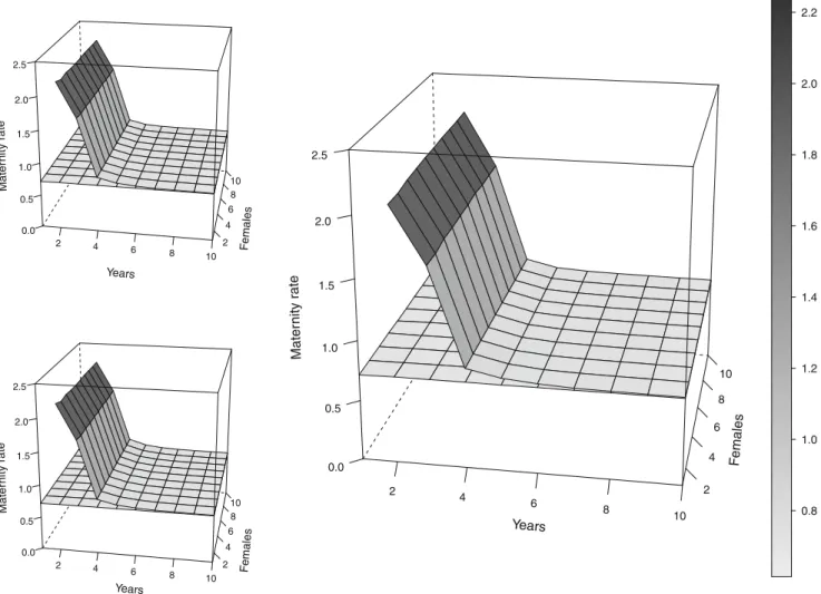
For the simulated unhunted population (Fig.1), the value of Mx computed from the alternative method M4 is consistent across numbers of monitoring years and numbers of monitored females at Mx00.72 (SD varying according to sampling
2 4 6 8 10 2 4 6 8 10 0.0 0.5 1.0 1.5 2.0 2.5 Years Females Mater n ity r a te 2 4 6 8 10 2 4 6 8 10 0.0 0.5 1.0 1.5 2.0 2.5 Years Females Mater n ity r a te 2 4 6 8 10 2 4 6 8 10 0.0 0.5 1.0 1.5 2.0 2.5 Years F emales Mater nity r ate 0.8 1.0 1.2 1.4 1.6 1.8 2.0 2.2
Fig. 1 Maternity rate Mx averaged estimates with simulated data for an unhunted population as a function of numbers of monitored years and females. Unit for maternity rate and on the gray scale is in cubs/ female/year. M1 top left, M2 bottom left, M3 right, M4 is the flat
surface shown on all figures. Note that methods M1, M2, and M3 cannot be used for study duration of 1 year. The exact correct value is Mx00.72 cubs/female/year
duration and sample size). By contrast, methods M1, M2, and M3 are upward-biased and duration-dependent. With method M3, a grizzly bear population of 10 females would, on average, have an Mx estimate of 1.69±0.53 if population was monitored during 3 years, 0.82±0.24 if population was monitored during 4 years, and 0.75±0.08 if population was monitored during 5 years. Varying the sample size of monitored females does not affect the bias introduced by methods M1, M2, and M3.
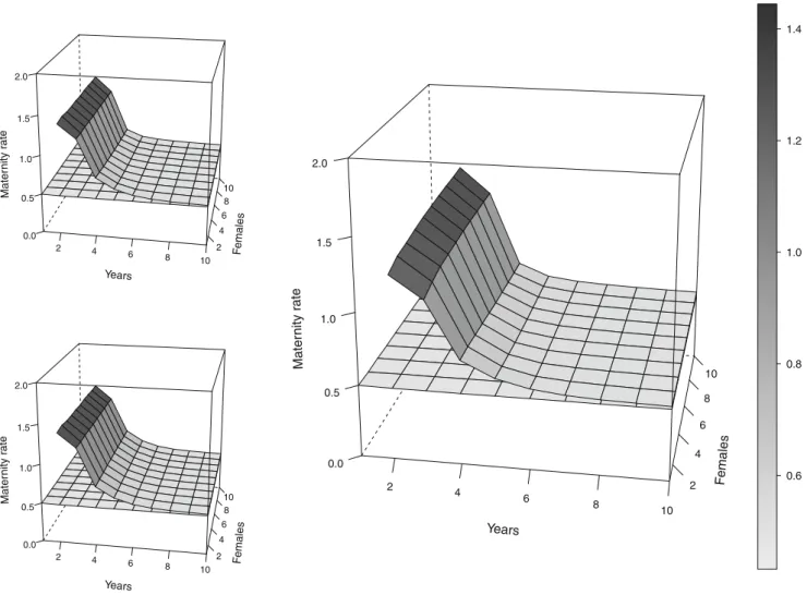
For the simulated hunted population, the bias is worse (Fig. 2). The value of Mx computed from the alternative method M4 is consistent across numbers of monitoring years and monitored females at Mx00.49 (SD varying according to sampling duration and sample size). By con-trast, methods M1, M2, and M3 are upward-biased and duration-dependent. With method M3, a grizzly bear popu-lation of 10 females would, on average, have an Mx estimate of 1.20±0.31 if population was monitored during 3 years, 0.66±0.20 if population was monitored during 4 years, and 0.57 ± 0.09 if population was monitored during 5 years.
Varying the sample size of monitored females does not affect the bias introduced by methods M1, M2, and M3.
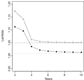
As a consequence of the upward bias in Mx, the standard method M3 overestimates population growth (Fig. 3). For the unhunted population monitored 3 years, method M3 returns a growing population (λ01.143), but the unbiased M4 method returns a much lower growth rate (λ01.049) and matches the true population growth rate. For the hunted population monitored over 3 years, method M3 returns a growing population (λ01.097), but the unbiased M4 meth-od indicates the population is stable (λ01.008) and matches the true population growth rate.
The bias in Mx using the standard M3 method increases with probability of unsuccessful pregnancies q0. For either the
unhunted or hunted population, the bias is nonexistent when this probability is 0, but reaches +10 % for q000.23, +25 % for
q000.43, and +50 % for q000.6 (hunted case on Fig.4). For
extremely unproductive populations (q000.8), method M3
overestimates Mx by 136 %. 2 4 6 8 10 2 4 6 8 10 0.0 0.5 1.0 1.5 2.0 Years Females Mater n ity r a te 2 4 6 8 10 2 4 6 8 10 0.0 0.5 1.0 1.5 2.0 Years Females Mater nity r a te 2 4 6 8 10 2 4 6 8 10 0.0 0.5 1.0 1.5 2.0 Years Females Mater nity r ate 0.6 0.8 1.0 1.2 1.4
Fig. 2 Maternity rate Mx averaged estimates with simulated data for a hunted population as a function of numbers of monitored years and females. Unit for maternity rate and on the gray scale is in cubs/female/
year. M1 top left, M2 bottom left, M3 right, M4 is the flat surface shown on all figures. Note that methods M1, M2, and M3 cannot be used for study duration of 1 year. The exact correct value is Mx00.49 cubs/female/year
Discussion
Our results indicates that methods M1, M2, and M3 yield overestimated, inconsistent, and duration-dependent estimates of Mx. Increasing the sampling duration to about 7–8 years would lower the bias. To completely eliminate the bias, all females in the sample would need to produce young, and the sampling duration would need to last an infinite number of years, which are both unrealistic. Increasing the sample size of monitored females does not decrease the bias. We agree that low precision is an important problem for low sample sizes; however, our point here is to show that even by considering that all individuals in a population could be observed, methods M1, M2, and M3 would still not return the correct value of maternity rate. We show that the bias from using the M3
standard method is a continuously growing function of the probability of unsuccessful pregnancies, and this method can therefore not detect a reduction of maternity rate due to an increase of unsuccessful pregnancies. By contrast, the M4 alternative yields unbiased estimates of Mx regardless of numbers of monitored females and duration of monitoring. In particular, method M4 does not introduce bias for data collected over short periods because it is not dependent on the existence of closed interbirth intervals; even though pre-cision at small sample size will be an issue (e.g., (Devenish Nelson et al.2010)).
The bias is greater in the unproductive, hunted popula-tions than in the productive, unhunted population for two reasons. First, the hunted population has a higher percentage of unproductive (no cubs) estrous females per year (20 vs. 12 %) and these “zero” females would be excluded in the method M3. Second, the hunted population has a smaller mean litter size, which has a higher probability of disappear-ing. Loss of a litter then results in more females moving to the estrous condition, and estrous females have a higher proba-bility of being a“zero” in the unproductive population.
We report estimates of Mx for each method as average values from 10,000 simulated datasets. Because our demo-graphic model is stochastic, it introduces a random variability in the data simulation process. For example, while averaged M4 estimates are a flat surface equal in all points to the correct value of Mx on Figs.1 and2, each individual M4 estimate from a single dataset may not necessarily be equal to the correct value—also the case for dataset obtained in real field conditions. However, this should not suggest an inaccuracy of method M4. As shown in Section 4 of the Supplementary Material, the density distribution of Mx estimates from method M4 is symmetrical and centered around the correct value (contrary to estimates from methods M1, M2, and M3), which reveals that the variation in Mx estimates from method M4 is not caused by any overestimating bias but simply by the stochasticity in the data.
These simulated results are consistent with the empirical data reported by Garshelis et al. (2005). They used the unbi-ased M4 method and reported an unexpectedly low Mx com-pared to other North American grizzly bear populations (0.24 vs. 0.32). They attributed their relatively low value of Mx due to some combination of real biological differences and/or bias in the other studies. We concur with Garshelis et al. (2005) that they found an unexpectedly small Mx and that the differences in estimated Mx were substantial—but the evidence presented here suggests that the main cause may be bias in other studies using the biased method M3 (Eberhardt et al. 1994; Hovey and McLellan1996; Miller1997), not an abnormally small Mx in their study area. We suspect that estimates of Mx reported in the literature using method M3, including our own previous work (Wielgus et al. 1994), may be biased overestimates. Despite a low elasticity of λ to Mx (Wielgus
2 4 6 8 10 0.95 1.00 1.05 1.10 1.15 1.20 Years Lambda
Fig. 3 Estimate ofλ when using Mx computed by method M3 with simulated data for hunted (black squares) and unhunted (empty circles) populations with 10 females as a function of monitoring duration. Pop-ulation growth rateλ computed with exact method M4 is 1.049 (unhunted population, dashed line) and 1.008 (hunted population, dotted line)
0.0 0.2 0.4 0.6 0.8 0 5 0 1 00 150
Probability of unsuccessful pregnancy
Ov
erestimate of Mx in %
Fig. 4 Overestimate b of Mx computed from its analytical expression derived in theMethodsSection, when using the M3 method (hunted population– continuous line, unhunted population – dashed line), as a function of probability of unsuccessful pregnancy q0
et al.2001), the bias was large enough to overestimateλ and have a stable, or even moderately declining, population con-sidered as a growing one.
These results suggest that previous reports of high popula-tion growth, λ01.08 (Hovey and McLellan1996), λ01.07 (Eberhardt et al. 1994), may be due to use of the biased estimates of Mx and not real gains in population numbers. For example, Wielgus and Bunnell (1994) and Wakkinen and Kasworm (2004) reported that the threatened Selkirk Mountain grizzly bears were stable and/or increasing, but both used the biased method M3. The results of the present paper suggest that the threatened Selkirk population may not be increasing towards recovery, but may be in fact, only stable or declining. The same conclusion may apply to the threatened Yaak population (Wakkinen and Kasworm2004)—it may be
declining much more rapidly than previously reported. Our results should incline researchers to abandon the use of the biased standard method M3 for species characterized by ex-tended parental care and instead to use the unbiased method M4 for population projections and assessments of population viability.
Acknowledgments Funding and support was provided by the Centre National de la Recherche Scientifique Laboratoire d’Ecologie; Museum National d’Histoire Naturelle Département Ecologie et Gestion de la Biodiversité; National Science Foundation; US Department of Energy, Bonneville Power Administration, Fish and Wildlife Program; Université d’Angers; Université Pierre et Marie Curie; Swedish University of Agricultural Sciences; and Washington State University.
References
Akçakaya HR, Burgman MA, Ginzburg LR (1999) Applied population ecology: principles and computer exercises using RAMAS EcoLab 2.0. Sinauer Associates, Sunderland
Boyce MS, Blanchard BM, Knight RR, Servheen C (2001) Population viability for grizzly bears: a critical review. International Association for Bear Research and Management - Monograph Series 4 Caswell H (2001) Matrix population models: construction, analysis,
and interpretation. Sinauer Associates, Sunderland
Chapron G, Quenette PY, Legendre S, Clobert J (2003) Which future for the French Pyrenean brown bear (Ursus arctos) population? An approach using stage-structured deterministic and stochastic models. Comptes Rendus - Biologies 326(suppl 1):S174–S182 Devenish Nelson ES, Harris S, Soulsbury CD, Richards SA, Stephens
PA (2010) Uncertainty in population growth rates: determining confidence intervals from point estimates of parameters. PLoS One 5(10):e13628. doi:10.1371/journal.pone.0013628
Eberhardt LL, Blanchard BM, Knight RR (1994) Population trend of the Yellowstone grizzly bear as estimated from reproductive and survival rates. Can J Zool 72(2):360–363
Garshelis DL, Gibeau ML, Herrero S (2005) Grizzly bear demograph-ics in and around Banff National Park and Kananaskis Country, Alberta. J Wildl Manag 69(1):277–297
Hovey FW, McLellan BN (1996) Estimating population growth of grizzly bears from the Flathead River drainage using computer simulations of reproduction and survival rates. Can J Zool 74 (8):1409–1416
Karanth UK, Stith BM (1999) Prey depletion as a critical determinant of tiger population viability. In: Seidensticker J, Christie S, Jackson P (eds) Riding the tiger: tiger conservation in human-dominated landscapes. Cambridge University Press, Cambridge, UK, pp 110–113
Kerley LL, Goodrich JM, Miquelle DG, Smirnov EN, Quigley HB, Hornocker MG (2003) Reproductive parameters of wild female Amur (Siberian) tigers (Panthera tigris altaica). J Mammal 84 (1):288–298
Lambert CMS, Wielgus RB, Robinson HS, Katnik DD, Cruickshank HS, Clarke R, Almack J (2006) Cougar population dynamics and viability in the Pacific Northwest. J Wildl Manag 70(1):246–254 Logan KA, Sweanor LL (2001) Desert puma: evolutionary ecology and
conservation of an enduring carnivore. Island Press, California Mace RD, Waller JS (1998) Demography and population trend of
grizzly bears in the Swan Mountains, Montana. Conserv Biol 12 (5):1005–1016
McLellan BN (1989) Dynamics of a grizzly bear population during a period of industrial resource extraction. III. Natality and rate of increase. Can J Zool 67(8):1865–1868
McLoughlin PD, Taylor MK, Cluff HD, Gau RJ, Mulders R, Case RL, Boutin S, Messier F (2003a) Demography of barren-ground griz-zly bears. Can J Zool 81(2):294–301
McLoughlin PD, Taylor MK, Cluff HD, Gau RJ, Mulders R, Case RL, Messier F (2003b) Population viability of barren-ground grizzly bears in Nunavut and the Northwest Territories. Arctic 56(2):185–190 Miller SD (1997) Impacts of heavy hunting pressure on the density and
demographics of brown bear populations in southcentral Alaska. Federal Aid in Wildlife Restoration, Research Final Report, Study 4.26, June 1997
Owen C, Niemann S, Slotow R (2010) Copulatory parameters and reproductive success of wild leopards in South Africa. J Mammal 91(5):1178–1187
Pease CM, Mattson DJ (1999) Demography of the Yellowstone grizzly bears. Ecology 80(3):957–975
Schwartz CC, White GC (2008) Estimating reproductive rates for female bears: proportions versus transition probabilities. Ursus 19(1):1–12 Schwartz CC, Keating KA, Reynolds Iii HV, Barnes VG Jr, Sellers RA, Swenson JE, Miller SD, McLellan BN, Keay J, McCann R, Gibeau M, Wakkinen WF, Mace RD, Kasworm W, Smith R, Herrero S (2003) Reproductive maturation and senescence in the female brown bear. Ursus 14(2):109–119
Thomson DL, Cooch EG, Conroy MJ (2008) Modeling demographic processes in marked populations. Springer, New York
Wakkinen WL, Kasworm WF (2004) Demographics and population trends of grizzly bears in the Cabinet-Yaak and Selkirk ecosys-tems of British Columbia, Idaho, Montana, and Washington. Ursus 15(1):65–75
Wielgus RB (2002) Minimum viable population and reserve sizes for naturally regulated grizzly bears in British Columbia. Biol Conserv 106(3):381–388
Wielgus RB, Bunnell FL (1994) Dynamics of a small, hunted brown bear Ursus arctos population in southwestern Alberta, Canada. Biol Conserv 67(2):161–166
Wielgus RB, Bunnell FL (2000) Possible negative effects of adult male mortality on female grizzly bear reproduction. Biol Conserv 93 (2):145–154
Wielgus RB, Bunnell FL, Wakkinen WL, Zager PE (1994) Population dynamics of Selkirk Mountain grizzly bears. J Wildl Manag 58 (2):266–272
Wielgus RB, Sarrazin F, Ferriere R, Clobert J (2001) Estimating effects of adult male mortality on grizzly bear population growth and persistence using matrix models. Biol Conserv 98(3):293–303 Williams BK, Nichols JD, Conroy MJ (2002) Analysis and
manage-ment of animal populations: modeling, estimation, and decision making. Academic, San Diego