Design of a film cooled MEMS micro turbine

Design of a film cooled MEMS micro turbine

by

Baudoin Philippon

Dipl6me d'ing6nieur, Ecole Polytechnique (June 1998)

Submitted to the Department of Aeronautics and Astronautics

in partial fulfillment of the requirements for the degree of

Master of Science in Aeronautics and Astronautics

at the

MASSACHUSETTS INSTITUTE OF TECHNOLOGY

May 2001

MASSACHUSETTS INSTITUTE OF TECHNOLOGY

SEP

11 2001

LIBRARIES

@ Massachusetts Institute of Technology 2001. All rights reserved.

rfr

Author ...

Certified by...

Certified by...

Department of Aeronautics and Astronautics

6::31

f

May 18, 2001

...

;-

...

Professor Alan H. Epstein

R. C. Maclaurin Professor of Aeronautics and Astronautics

Thesis Supervisor

.. . . . . . . . . ... . . . . . . .. . . .

I/ T YDr Chon Tn

Senior Research Scientist, Gas Turbine Laboratory

Thesis Supervisor

Design of a film cooled MEMS micro turbine

Baudoin Philippon

Submitted to the Department of Aeronautics and Astronautics on May 18, 2001, in partial fulfillment of the

requirements for the degree of

Master of Science in Aeronautics and Astronautics

Abstract

As part of an effort to develop a portable power generation system, a fluid dynamics and ther-mal transfer investigation of a micro radial inflow turbine was carried out.

The 3-D numerical performance assessment revealed that the baseline 2-D designed turbine stage was not matched to the baseline compressor, resulting in off design operation. The CFD pre-dicts that the baseline turbine has a total to static efficiency of 29%, and does not provide enough power to drive the compressor at the matched pressure ratio of 1.65. Reasons for this low efficiency are the blockage due to end walls effects and to the exit right angle turn, and 3-D secondary flows in the blade passage leading to boundary layer separation.

The turbine was then redesigned. An analytical design procedure, based on a mean line analysis and correlations from 3-D CFD solutions was formulated and validated against numerical results. It was shown that significant performance gains could be achieved by increasing the turbine exit area to reduce the exit viscous loss and by increasing the blade exit angle. Shaping of the exit diffuser turned out not to be viable because of the difficulties in keeping the boundary layer attached. An improved turbine was then designed. Numerical simulations of the improved design predicted a 20% gain in efficiency, at a matched pressure ratio of 2.1.

Still, the turbine cannot drive the compressor. The turbine is conduction cooled by the com-pressor, but the large heat addition to the compressor flow causes a 30% drop in efficiency. Film cooling schemes for the turbine were investigated. An axisymmetric model showed that a coolant layer flowing radially inward may sustain the adverse centrifugal force at design speed. Film cooling schemes were then proposed for disk and blade cooling. Effectiveness drivers are surface coverage, thermal mixing with the main flow, and coolant matching. The overall peak cooling effectiveness of the proposed cooling schemes was approximately 30% for a 30% coolant flow.

Thesis Supervisor: Professor Alan H. Epstein

Title: R. C. Maclaurin Professor of Aeronautics and Astronautics Thesis Supervisor: Dr. Choon S. Tan

Acknowledgments

I would like to express my gratitude to Prof. Alan Epstein for his encouraging support, and for his many insightful suggestions throughout this project. By allowing me to work in this micro engine project as the "turbine guy" for two years, he gave me a challenging position and a lot to learn I also wish to thank Dr. Choon Tan for his constant encouraging support. His valuable guidance, direction, and insistence through the course of this research are much appreciated. In addition, I would like to acknowledge the guidance of Dr. Yifang Gong, and thank him for his help and his suggestions which lead to many improvements in the project.

Finally, I would like to thank all people of the micro engine project for making the past couple of years a memorable experience as a foreign student at MIT. I will definitely recommend this kind of experience!

This work was sponsored by the United States Army Research Office and the Defense Advanced Researched Project Agency.

Contents

1 Introduction

1.1 Background . . . . 1.2 The MIT Micro Engine ... ...

1.3 Challenges for the Turbomachinery . . . . 1.4 Goals and Content of the Thesis . . . .

1.5 Contribution of the Research . . . . 2 Assessment of the Baseline Turbine Stage

2.1 Consistency of the boundary conditions set . . . . .

2.2 Exploration of the Design Space . . . . 2.3 End Wall and 3-D Effects Dominate over 2-D Flow . 2.4 1-D Design Procedure using 3-D Simulations Results

2.4.1 Outline of Design Approach . . . . 2.4.2 1-D Design Procedure Validation . . . .

3 Design Improvement Techniques

3.1 Increasing Turbine Exit Area . . . .

3.2 Increasing NGV Turning . . . .

3.3 Exit Diffuser Shaping . . . .

3.4 Comparison of Baseline and Improved Turbine Stage 3.4.1

3.4.2 3.4.3

Presentation of the Baseline and Improved Turbine Stage Comparison at Expected Operating Point . . . . Comparison of Performance Maps . . . . 4 Cooling Studies

4.1 Cycle Analysis with Conduction Cooling only . . . . 4.1.1 Cycle Analysis . . . . 4.1.2 Discussion on Heat Transfer Predictions . . . . 4.2 Primary Study of Film Cooling: Risks and Potential Effectiveness 4.2.1 General Considerations on Film Cooling . . . . 4.2.2 Coolant Layer Centrifugation on a Rotating Disk (2-D)

4.2.3 Effectiveness of Disk Film Cooling (2-D CFD) . . . .

4.2.4 Effectiveness of Blade Film Cooling (2-D CFD) . . . .

4.3 Detailed Study of Disk Film Cooling (3-D CFD) . . . .

(2-11 11 11 12 14 15 16 17 19 20 25 25 28 31 31 32 36 38 39 40 43 51 51 51 52 55 55 59 63 66 71 D

.

.

.

4.3.1 Advantages and Disadvantages of Injection from the Static Structure and from the R otor . . . . 4.3.2 Disk Cooling with Injection from the Static Structure . . . . 4.3.3 Disk Cooling with Injection from the Rotor . . . .

5 Conclusion and Recommendations

5.1 Conclusions on Performance Improvements and Film Cooling . . . .

5.2 Future W ork . . . . A Validation of Fluent

A .1 The Fluent Code . . . . A.1.1 The Segregated Solver . . . .

A.1.2 The Coupled Solver . . . . A.2 Validation in 2-D (Turbine Geometry) . . . .

B Discussion on the Effect of the Journal Bearing Flow

C Discussion on Typical Flow Features in the Micro Turbine C.1 Flow in the NGV for an Inlet Pressure of 2.1 atm . . . . C.2 Flow in the Rotor for an Inlet Pressure of 1.8 atm . . . . C.3 Flow in the Rotor Matched to the Compressor . . . .

72 72 81 90 90 92 94 94 95 96 96 98 101 103 104 106 . . . . . . . . . . . .

List of Figures

1-1 Cross-section of the demo-engine . . . . 12

1-2 Picture of an early version of the baseline geometry turbine (October 1999 geometry) 13 2-1 3-D rotor calculations performed viewed in a Reynolds-Rossby number design space 20 2-2 2-D/3-D exit loss coefficient in the nozzle guide vanes (400 pm height, baseline design) vs. exit Reynolds number . . . . 21

2-3 NGV loss coefficient for 3 different wall shear conditions . . . . 23

2-4 Axial Mach number at the turbine exit annulus after the right angle exit turn (base-line design) . . . . 24

2-5 Description of the iterative turbine stage design . . . . 26

2-6 Correlation for the NGV loss coefficient . . . . 29

2-7 Correlations for loss coefficient at the turbine exit right angle turn . . . . 30

3-1 Parametric study: turbine stage efficiency vs. rotor exit radius (NGV turning con-stant at 74 degrees) . . . . 33

3-2 Fraction of the exit area used for exit mass through flow . . . . 33

3-3 Parametric study: NGV turning vs. turbine stage efficiency (Rotor exit radius constant at 2.0 m m ) . . . . 35

3-4 Parametric study: NGV turning vs. turbine mass flow (Rotor exit radius constant at 2.0 m m ) . . . . 36

3-5 Schematic of the turbine rotor with a shaped exit diffuser . . . . 38

3-6 Perspective of the grid for baseline nozzle guide vane . . . . 40

3-7 Perspective of the grid for baseline turbine rotor (top) and improved turbine rotor (bottom ) . . . . 41

3-8 Top view of the baseline turbine stage (top) and the improved turbine stage (bottom) (outer diameters of the rotor and stator are indicated) . . . . 42

3-9 Baseline stage (top) and improved stage (bottom): shaft work and loss distribution at the predicted operating point . . . . 44

3-10 Performance map: efficiency contours of baseline design (top) and improved design (bottom ) . . . . 46

3-11 Relative velocity vectors at mid span, for the improved rotor, at PR = 1.55 and 120% design speed . . . . 47

3-12 Performance map: shaft work contours (reference = 80 W) of baseline design (top) and improved design (bottom) . . . . 48

3-13 Performance map: disk Stanton number contours of baseline design (top) and im-proved design (bottom ) . . . . 49

3-14 Performance map: blade Stanton number contours of baseline design (top) and im-proved design (bottom ) . . . . 50

4-1 Normalized heat flux in the turbine rotor for various designs (see equation 4.3) . . . 52

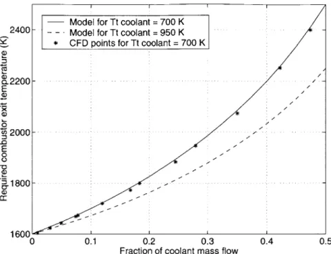
4-2 Required combustor exit temperature to reach a mass-average inlet total temperature

of 1,600 K with a cooling scheme . . . . 58

4-3 Minimum Rossby number to avoid coolant centrifugation of a cold film on a rotating disk, inlet total temperature 1600 K . . . . 61

4-4 Minimum Rossby number to avoid coolant centrifugation of a cold film on a rotating disk, inlet total temperature 1800 K (thin lines are Ttiniet = 1,600 K, figure 4-3) . . 62

4-5 Schematic of the 2-D axisymmetric geometry . . . . 63

4-6 Cooling effectiveness of radial injection over a 2-D rotating disk . . . . 65

4-7 Schematic of the 2-D axisymmetric geometry with a 15 p m step between the vanes exit and the rotor inlet . . . . 66

4-8 Cooling effectiveness of radial injection over a 2-D rotating disk with a 15 pm step) . 67

4-9 View of the improved blade with coolant injectors at the leading edge . . . . 69

4-10 Pressure surface blade cooling: isothermal cooling effectiveness and required coolant pressure for a 30 pm slot . . . . 70

4-11 Suction surface blade cooling: isothermal cooling effectiveness and required coolant pressure for a 30 pm slot . . . . 71 4-12 Blade cooling: turbine work variation due to coolant injection . . . . 72

4-13 Required compressor pressure to inject coolant at 77 degrees matched to the im-proved turbine . . . . 76

4-14 3-D cooling effectiveness ON THE ROTOR for 3 coolant injection conditions (radial,

77 degrees, 77 degrees high pressure) . . . . 77

4-15 3-D cooling effectiveness ON THE DISK for 3 coolant injection conditions (radial,

77 degrees, 77 degrees high pressure) . . . . 78

4-16 3D cooling effectiveness ON THE BLADES for 3 coolant injection conditions (radial,

77 degrees, 77 degrees high pressure) . . . . 79

4-17 3-D cooling effect on shaft work for 3 coolant injection conditions (radial, 77 degrees,

77 degrees high pressure) . . . . 80

4-18 3-D cooling effectiveness ON THE DISK for 77 degree injection, for coolant temper-atures equal to 700 K, 900 K, and 1100 K . . . . 82

4-19 Top view of a blade passage with first cooling slot geometry . . . . 84 4-20 Top view of a blade passage with second cooling slot geometry . . . . 85

4-21 Disk cooling effectiveness ON THE ROTOR of two cooling configurations with in-jection from the disk . . . . 86

4-22 Disk cooling effectiveness ON THE DISK of two cooling configurations with injection

from the disk . . . . 87

4-23 Disk cooling effectiveness ON THE BLADES of two cooling configurations with injection from the disk . . . . 88

4-24 Shaft work variation of two cooling configurations with injection from the disk . . . 89 5-1 Disk cooling injection from the rotor, with an additional cover plate to turn the

B-1 Impact of the journal bearing flow on the turbine rotor efficiency (Baseline design) . 100 B-2 Cooling effectiveness of the flow coming from the journal bearing (Baseline design).. 100

C-1 Reversible term of entropy in the NGV, for the baseline design (left) and improved

design (right), at 2.5% span (top), 50% span (middle), and 97.5% span (bottom), for an inlet pressure of 2.1 atm . . . 107

C-2 Irreversible term of local entropy production in the NGV, for the baseline design

(left) and improved design (right), at 2.5% span (top), 50% span (middle), and

97.5% span (bottom), for an inlet pressure of 2.1 atm . . . 108 C-3 Total pressure in the NGV, for the baseline design (left) and improved design (right),

at 2.5% span (top), 50% span (middle), and 97.5% span (bottom), for an inlet pressure of 2.1 atm . . . 109 C-4 Total temperature in the NGV, for the baseline design (left) and improved design

(right), at 2.5% span (top), 50% span (middle), and 97.5% span (bottom), for an inlet pressure of 2.1 atm . . . 110

C-5 Mach number in the NGV, for the baseline design (left) and improved design (right),

at 2.5% span (top), 50% span (middle), and 97.5% span (bottom), for an inlet pressure of 2.1 atm . . . .111

C-6 Path lines in the NGV, for the baseline design (left) and improved design (right),

starting at 2.5% span (top), starting at 50% span (middle), and starting at 97.5% span (bottom), for an inlet pressure of 2.1 atm . . . 112

C-7 Normalized absolute swirl in the rotor, for the baseline design (left) and improved

design (right), at 2.5% span (top), 50% span (middle), and 97.5% span (bottom), for an inlet pressure of 1.8 atm . . . 113

C-8 Reversible term of entropy in the rotor, for the baseline design (left) and improved

design (right), at 2.5% span (top), 50% span (middle), and 97.5% span (bottom), for an inlet pressure of 1.8 atm . . . 114

C-9 Irreversible term of local entropy production in the rotor, for the baseline design (left)

and improved design (right), at 2.5% span (top), 50% span (middle), and 97.5% span (bottom), for an inlet pressure of 1.8 atm . . . 115

C-10 Static pressure in the rotor, for the baseline design (left) and improved design (right),

at 2.5% span (top), 50% span (middle), and 97.5% span (bottom), for an inlet pressure of 1.8 atm . . . 116

C-11 Static temperature in the rotor, for the baseline design (left) and improved design

(right), at 2.5% span (top), 50% span (middle), and 97.5% span (bottom), for an inlet pressure of 1.8 atm . . . 117

C-12 Path lines in the rotor, for the baseline design (left) and improved design (right),

starting at 2.5% span (top), starting at 50% span (middle), and starting at 97.5% span (bottom), for an inlet pressure of 1.8 atm . . . 118

C-13 Swirl relative to inlet (top), local irreversible entropy production (middle), and static

pressure contours (bottom) for the baseline rotor (left) and the improved rotor (right) at their respective matched operating point (see table 3.2) . . . 119

List of Tables

2.1 Geometrical parameters explored . . . . 27

2.2 Operating parameters explored . . . . 27

3.1 Summary of design characteristics of the baseline turbine design and the improved stage... ... 39

3.2 Summary of stage performance of the baseline and improved design . . . . 43

3.3 Reference and design quantities for the turbine maps . . . . 44

4.1 Physical scales used in dimensionless equations . . . . 59

4.2 Advantages and disadvantages of coolant injection from a static or rotating structure 73 4.3 Boundary conditions for the coolant layer, in the three disk cooling cases with injec-tion from the static structure . . . . 75

A.1 Fluent 2-D/MISES comparison for baseline NGV . . . . 97

Nomenclature

Roman

Loss coefficient (dimensionless), defined as C, = _{Pt out -P}in

jPt

~t

Mass flow (g.s 1

) Static pressure (Pa)

Heat transfer, positive to the fluid (W)

Reynolds number (dimensionless), based on the specified length and location Static temperature (K)

Vector position

Ratio of the total pressure at the rotor inlet to a total pressure of reference Rotation speed (rad.s-1₎

Ratio of the total temperature at the rotor inlet to a total temperature of reference

In the absolute non-rotating frame

At the engine exit, after the exhaust right angle At the inlet

At the blade trailing edge In the rotor rotating frame

Total quantity in the absolute frame

Denotes a quantity on the wall surface, either blade or end wall

CI M rh P

Q

u

Greek

Subscripts

Chapter 1

Introduction

1.1

Background

Advances in micro machining techniques have lead to the development of numerous Micro Electro-Mechanical Systems, known as MEMS, with applications in virtually every scientific field such as medicine, electronics or aeronautics. Specifically, the current development of micro-scale power generation systems demonstrate new directions in concepts for portable, disposable and low cost systems.

An MIT program proposes to demonstrate the feasibility of a micro gas turbine engine. Based on a Brayton cycle, this micro engine benefits from the square-cube law: at the scale of a shirt button, its power density could be an order of magnitude larger than conventionally sized gas turbine engines (Epstein et al [3]).

Applications include portable power generation (with a power density twenty times that of batteries), micro blowers and compressors, micro rocket engines, and propulsion for micro air vehicles. The effort is supported jointly by the Army Research Office and the Defense Advance Research Project Agency (DARPA).

1.2

The MIT Micro Engine

Although based on the same fundamental principles, the MIT micro-engine cannot simply mimic conventional gas turbine engines since it must take into account specific issues related to the micro

Starting

Air In Compressor Inlet

3.7 mm

Exhaust Turbine Combustor

21 mm

Figure 1-1: Cross-section of the demo-engine

scale of the device. The original baseline design is presented in Epstein et al [4]. Calculations showed that such a micro gas engine could produce up to 50 W of electrical power for portable power generation, or 0.2 N of thrust for a micro air vehicle.

The general approach of the engine is close to that of the first jet engines in the late fourties and to current auxiliary power units. The micro engine consists of a single stage centrifugal compressor, an annular combustor and a radial inflow turbine to spin the compressor and provide extra power for the output (as shaft torque). Because of the required rotational speed, the rotor is supported on air bearings. Two thrust bearings support the thrust load along the longitudinal axis and a journal bearing supports the radial rotor load. A detailed discussion of the operating modes of the journal bearing can be found under Piekos et al [10]. A cross sectional view of the baseline engine is presented in figure 1-1. A photo of the baseline turbine is shown in 1-2.

1.3

Challenges for the Turbomachinery

At this size, thermodynamics is the same as for conventional gas turbine engines, but mechanics and thus the optimum design trade-offs do change with scale. Moreover, fabrication constraints in the micro scale prevent simply scaling down conventional turbomachinery. Design studies have demonstrated the governing micro engine parameters, pointing out where they differ from those of conventional engines. The work to date has emphasized the following points:

e Centrifugal stress at the turbine blade roots dominates but is compatible with the choice of

silicon and silicon carbide for fabrication reasons. The softening temperature of silicon at the design rotation speed of 1.2 million RPM is 950 K, so the turbine rotor temperature must be

maintained below this level.

" Very low Reynolds number is not a barrier to break-even. It was shown, using

computa-tional analysis and experimental data, that the design of turbomachinery components with acceptable adiabatic efficiency was possible. Still, as the Reynolds number in the compressor reaches 25,000 and 1,500 in the turbine, its influence remains strong and any improvement in the cycle pressure ratio leads to significant gains in component efficiency.

" Fabrication restricted to pure 2-D extrusion is a direct consequence of the micro machining

techniques chosen. It precludes 3-D shape optimization, while all out-of-plane flow turns must be right angles, which produces significant blockage and viscous loss.

" Large heat fluxes derive from the small scale and high thermal conductivity of the material.

To maintain the turbine rotor temperature below 950 K, it is currently cooled by thermal conduction to the compressor. But this heat addition drastically reduces the compressor performance, a major parameter in a turbojet efficiency and power output. So, other tech-niques must be explored to maximize turbine gas temperature while limiting heat flux to the

compressor.

1.4

Goals and Content of the Thesis

The goals of this thesis are to explore the turbine design space, to determine the parameters governing turbine efficiency and heat flux, and then to propose a new film cooled turbine design with improved component efficiency.

The second chapter presents the initial design space exploration: the analysis performed on the nozzle guide vanes and the turbine rotor concluded that viscous loss on end walls are an important design factor (section 2.3). A new design procedure is introduced to remedy the short comings of the previous 2-D only design procedure (section 2.4).

The third chapter focuses on using the new design procedure to realize improved designs. The baseline design is compared with an improved design proposed for fabrication (section 3.4).

The fourth chapter deals with heat transfer in the micro engine, and presents a risk and per-formance analysis of film cooling on both the turbine disk and the turbine blades.

The last chapter presents the summary and conclusions of the research, as well as recommen-dations for future work.

1.5

Contribution of the Research

The research presented in this thesis has taken several steps in the development of the micro engine turbine design:

e

designs presented in the third chapter. They can be used in cycle and systems analysis and are provided as a "best guess" as no experimental data is yet available. It was shown that matching issues lead to unacceptable performance of the baseline design.

e

Based on mean line analysis and 3-D CFD experience, the model was used to improve the component efficiency by more than 20% to bring it up to 55%, closer to the expected turbine performance in the early cycle studies.

e

addi-tion to the compressor. It is shown that reverse flow in the coolant layer due to centrifugal forces is not a limit in the planned operating range, and that turbine disk cooling can be very effective if sufficient coolant pressure is available.

Chapter 2

Assessment of the Baseline Turbine

Stage

The baseline turbine was designed and optimized in 2-D by Harold Youngren [2]using a numer-ical code called MISES (Multiple blade Interacting Stream tube Euler Solver). This code creates a 2-D mesh on a stream tube around the blades given by an inviscid Euler analysis, then uses the boundary layer theory to compute the flow near the blade surface.

Then we performed a 3-D analysis of this design using a 3-D Reynolds averaged, steady, Navier-Stokes solver called Fluent (presentation and validation of this code is in appendix A). We found that the 2-D designed components were seriously mismatched in 3-D, due to end walls effects and blockage at the exit right angle turn. Unmatched components result in off design operation of the blade rows, which can drop turbine performance and engine efficiency. So this chapter discusses the CFD analysis of the baseline turbine stage design with particular attention to the issue of tur-bine matching.

First, we discuss boundary conditions chosen for consistency set for each blade row. Confidence in the numerics are then generated through an exploration of the design space. The next section shows that end wall effects are dominant in the demo engine for etch depths up to 400 im. Last, an alternative design method, based on mean line analysis with correlations from 3-D numerical solutions, is explained and validated.

2.1

Consistency of the boundary conditions set

The performance estimation rests on several crucial considerations to provide accurate and con-sistent results within the scope of the chosen assumptions. A validation study has been performed to gain confidence in the 3-D, Reynolds averaged, Navier-Stokes numerical tool, Fluent. Both the code description and the validation study can be found in appendix A.

Also important are the boundary conditions used in the calculations and the understanding of how they impact the final accuracy.

The first group summarizes the matching effort undertaken throughout this research and are a basic requirement for accuracy.

" Pressure matching. We mean by that the total pressure at the NGV exit is equal to the total

pressure at the rotor inlet. Those values have to be precisely matched at a constant radial plane (r = 3mm).

" Mass flow matching. We also demand the mass flow in the NGV to be equal to the mass flow

in the rotor. As calculations for the NGV and the rotor are done independently, we need to iterate on the NGV inlet total pressure and on the NGV exit static pressure to match the rotor mass flow. Practically, this is done using interpolations among at least four NGV cases

(two NGV inlet conditions and two NGV outlet conditions).

" Temperature matching. The temperature at the vane exit is equal to the temperature at

the rotor inlet. This requirement is approximately respected in the simulations, where to-tal temperatures are imposed at the NGV inlet and rotor inlet. Adiabatic calculations are performed in the NGV for several reasons. First, the NGV viscous loss does not decrease drastically with heat transfer, so adiabatic calculations overestimate only slightly the NGV pressure loss. Second, the total temperature does not change throughout the NGV passage, so we don't have to iterate on the NGV inlet total temperature until the NGV exit reaches the required 1,600 K. So, using adiabatic calculations in the NGV saves computer time while providing realistic results for the matching process.

the required number of different operating conditions. It was applied to the total pressure between the nozzle guide vanes exit and the rotor inlet, to the turbine shaft work and to the heat flux to the turbine wall.

Compressor matching. Matching the compressor means matching the rotation speed, the

mass flow, the pressure ratio, and the power. In the design procedure suggested later in this chapter, the aim is to match the rotation speed, the pressure ratio and the mass flow and to design a turbine rotor with the highest possible efficiency. As described in the next chapter, this is insufficient: the power required by the compressor is still not balanced by the turbine power. Reducing the heat flux to the compressor is necessary. At this point, the cycle analysis is more complex and is not treated herein.

The second group deals more with assumptions used to reduce the numerical work load. It is true that higher precision may result if the following assumptions were not made, but the goal of the research is to obtain governing parameters and general trends rather than to reach a precision expensive both in time and computer resources. The assumptions are:

" Steady calculations provides sufficiently good performance estimations for design purposes.

On the other hand, this ignores unsteady phenomena such as wake-blade interaction. But we do not expect this to be an important factor given the expected accuracy of the calculations and the required performance of the turbine stage.

" Uniform inflow conditions were stipulated at boundaries. When the outflow of one simulation

was used as input in another, total quantities and tangential velocity were mass-averaged while static quantities and radial velocity were area-averaged. To validate this assumption, a

complete simulation of the turbine stage was performed. The flow quantities at the interface between the NGV and the rotor were circumferentially averaged by the code, so the rotor inlet conditions were non uniform in the longitudinal direction. The full stage efficiency was only 2% lower than the efficiency predicted using uniform inflow conditions for the rotor. We will generalize this to all results presented in the thesis.

" No boundary layers were specified at the domain inlet. Instead, the computational domain was

and allow for an onset of viscous and thermal boundary layers. Due to the higher shear near a boundary layer starting point, we can expect both the viscous loss and the heat flux to be overestimated by this technique.

To assess the accuracy of these performance predictions, we consider the impact of:

* NGV-rotor flow temperature matching. Currently, only pressure and mass flow are matched

precisely, so that there is a temperature discontinuity between the nozzle guide vanes and the turbine rotor: the computed total temperature at the NGV exit is approximately 10% lower than the total temperature imposed at the rotor inlet. Consequently, the "matched" point would be at a slightly lower mass flow, the total pressure between the NGV and rotor being also reduced. Because the total temperature drop in the NGV is due solely to heat transfer to the static structure, and heat transfer depends linearly on the temperature difference between the wall and the inlet, improved estimates for the wall temperatures would be needed.

" Flow from the journal bearing. There is a 15 micron wide gap between the NGV exit and the

rotor inlet, through which approximately 5% of the main flow passes at design speed. This

flow, which is studied in appendix B, reduces the turbine performance in two ways. First, it

leaves the journal bearing gap at an angle of 90 degrees to the main flow, thus disrupting the boundary layers and mismatching the rotor blades inlet flow angle. Second, as its temperature is lower than the main flow (between the estimated static structure temperature of 1,200 K and the rotor temperature of 950 K), less work can be extracted from this cold layer than from the turbine main flow. In our performance estimations, a correlation of shaft work reduction versus the fraction of the flow coming from the journal bearing has been calculated in 3-D and used thereafter.

2.2

Exploration of the Design Space

The design space has conceptually a large number of dimensions, so it is truly impossible to present it on a two dimensional sheet of paper. Even in the limited scope of this research, many ideas have been explored (some unsuccessfully) in aerodynamic performance and cooling.

+ * * + 4 + * + + ++ + ++ * + +, * * * * * 0

0

Reynolds number (based

1

on inlet conditions)

Figure 2-1: 3-D rotor calculations performed viewed in a Reynolds-Rossby number design space

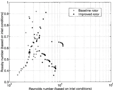
and Rossby number (presented in appendix A). Major calculations are shown in figure 2-1. The points are fairly well distributed indicating an effort to simulate the flow under various conditions.

A shift of Reynolds number to higher values to the right is visible from the baseline rotor to the

improved rotor. It is due essentially to the improved compressor design and improved matching, which resulted in a higher total pressure available at the rotor inlet, thus increasing Reynolds num-ber.

To illustrate the work done and point out several flow features, some calculations are presented in appendix C.

2.3

End Wall and 3-D Effects Dominate over 2-D Flow

Early calculations showed that the mass flows predicted in 3-D were generally 30 to 40% lower than those predicted in 2-D. This pointed out the need for metrics to measure the blockage and

0.5. CD 0I) N 0 C W 0.3 0 %0. 0 (0 0 Lii 0.1 103

Exit Reynolds number

Figure 2-2: 2-D/3-D exit loss coefficient in the nozzle guide vanes (400 pm height, baseline design) vs. exit Reynolds number

viscous loss due to low Reynolds number in the nozzle guide vanes and the turbine rotor.

First, for the blockage due to viscous loss in the nozzle guide vanes, a loss coefficient was defined as follows:

C= Pt in-Ft out (2.1)

Pt out - Pout

This represents the total pressure drop in the nozzle guide vanes (due to viscous loss) over the dynamic pressure at the passage exit (radius r = 3 mm).

Results are shown in figure 2-2, where the loss coefficient of the baseline NGV obtained with Fluent in 2-D and 3-D are compared. As shown in the validation process in appendix A, MISES and Fluent in 2-D are in excellent agreement. So for 2-D calculations, Fluent has been chosen to make a fair back-to-back comparison.

In conventional modern turbines, the level of loss in 3-D is approximately 3 times higher than

*-- 3D loss coefficient - - 2D loss coefficient F F -- I-- -~ + 1-.. ... .... 10 4

that in 2-D. In our case, the factor is closer to 4 in this back-to-back comparison, prompting the need for further analysis to determine the source of the higher loss: the boundary layer on the blade surface, the boundary layer on the end wall surface, or the interaction of the two.

In numerical simulation, it is possible to set a no-shear condition on one wall independently of the other, so that we were able to compute the viscous loss due solely to the blade surface and solely due to the end wall surface. Figure 2-3 shows the 3-D computed loss coefficients.

Clearly, viscous loss on end walls is dominant. They represent roughly 2/3 of the loss in the nozzle guide vanes. The fact that the sum of the loss coefficients for viscous end walls only and viscous blade only approximates the total loss coefficient suggests that the interaction between the two boundary layers is not an important factor. Strong secondary flow is observed on the NGV blade surface. We can conclude they are due to the strong pressure gradient in the blade passage influencing the end wall boundary layers. Increasing the etch depth above 400 microns would help reduce this secondary flow and the associated 3-D loss.

The other dominant source of blockage is the right angle, out-of-plane turn downstream of the rotor exit. As mentioned in the introduction, manufacturing constrains the design to 2-D etching, so that all turns in the longitudinal axis are right angles. This sharp, right angle turn separates the boundary layer, which produces significant recirculation and flow blockage.

To assess the reduction of effective exit area, we examine the axial Mach number at the turbine exit, after the right angle turn. Figure 2-4 shows the exit Mach number of the baseline turbine, operating close to the predicted matched operating point (PR = 1.65). The axial Mach number

is at least 20% lower than its maximum value in the dark area, and is even negative in regions of reverse flow indicating a recirculation near the turn. In the baseline case, the effective area is

30% lower than the physical flow area. It will be shown in section 3.1 in the next chapter that

the effective area is even smaller in the improved turbine while the right angle turn causes fewer loss.

Since the baseline design, based on 2-D CFD, does not take into account these 2 sources of blockage, the mass flow we can expect in 3-D and in the experiment will be significantly lower than the nominal design value. Thus, the velocity triangles are largely off-design, both for the compressor and the turbine. For instance, the predicted turbine efficiency in 3-D with Fluent is

0.3 C 60.2 0 CO) CD 0 x w 0.1

End wall and blade viscous Viscous end wall only Viscous blade only

Figure 2-3: NGV loss coefficient for 3 different wall shear conditions

0.5 0.4 0.3 0.2 0.1 -0.0 -0.1 -0.2 -0.3 Figure 2-4: Axial Mach design)

30% at this operating point, instead of approximately 60% predicted by MISES.

For this reason, there is a need for another design procedure, resting more on a prediction of the blockage to yield the desired velocity triangles. 3-D CFD provides such a prediction capability

(2-D CFD may be sufficient for the right angle turn). This is the objective of the next section.

2.4

1-D Design Procedure using 3-D Simulations Results

The proposed design procedure is simple. It is based on a mean line analysis (as described in Kerrebrock [9]), computing pressures, temperatures and velocities at each station: NGV inlet,

NGV outlet, rotor inlet, rotor outlet, and stage exit.

However, 3-D effects must be taken into consideration early in the design process, so they are included either as correlations from 3-D solutions or best guesses. The result of this is an iterative algorithm which computes the stage mass flow, the rotor blade leading edge and trailing edge angles, specified operating conditions (total pressure and total temperature at the turbine stage inlet, static pressure at the turbine stage outlet, rotation speed).

In the following sections, the design procedure is described and validated.

2.4.1 Outline of Design Approach

Figure 2-5 depicts the user inputs and the iterative process. The procedure is flexible, because many geometrical and operational inputs can be chosen. So parametric studies can be performed on any parameter or set of parameters.

The geometrical inputs are summarized in table 2.1. The operational inputs are shown in table 2.2. Typically, one wants to design a turbine stage given some operational requirements such as those specified in the second table. So the optimization is carried out mostly on the geometrical parameters.

It should be noted first that most operational parameters can be updated as experience builds, so that the procedure accuracy can increase with time. Second, a rotor passage efficiency is required: it represents the total to total isentropic efficiency of the blade passage only, excluding effects such as the exit right angle turn. It turns out that this efficiency is fairly constant. The rotor efficiency predicted in 2-D is a good first guess for this parameter.

Set stage geometry

(Blade height, inlet and exit radii, NGV turning)

I

Set stage flow conditions

(tinlet' inlet' outlet

Assume inlet mass flow

I

I

NGV loss coefficient = f(Reynolds or NGV turning)

(From 3D CFD)

Determine velocity triangles

(Rotor efficiency from 3D experience)

Exit loss = f(exit Mach number)

(From 3D CFD)

Determine outlet pressure

I

I

ZZIEIZ

I

Turbine stage performance

Figure 2-5: Description of the iterative turbine stage design

I

h..- I

PP-

_I

I

I

I

Parameter Value or range

NGV blade height (pim) 400

NGV inlet radius (mm) 4.8

NGV outlet radius (mm) 3.04

NGV leading edge angle (degree) 0

NGV trailing edge angle (degree) 60-85

Rotor blade height (pm) 400

Rotor inlet radius (mm) 1.5-3

Rotor outlet radius (mm) 1.5-3

Table 2.1: Geometrical parameters explored

Parameters Value or range

Stage inlet total pressure (atm) 1.5-3

Stage inlet total temperature (K) 1,600

NGV loss coefficient (-) Correlation

NGV heat transfer estimation (W) 60

Rotor speed (RPM) 1.2 million

Rotor passage adiabatic efficiency (-) 0.75

Rotor deviation (degree) 0-20

Rotor heat transfer estimation (W) 60

Viscous loss of the exit right angle turn (-) Correlation Stage exit static pressure (atm) 1

2.4.2

1-D Design Procedure Validation

In table 2.2, two important parameters require a correlation: the nozzle guide vane loss and the exit right angle turn loss. Those correlations have been established using a number of CFD cases.

For the NGV loss coefficient correlation presented in figure 2-6, different vane geometries were drawn and simulated in 3-D with Fluent. The correlation adopted for the design procedure captures the trend of increasing loss with increased turning to the first order. The fact that the loss coefficient increases again at angles close to 60 degrees may mean that more cases would be required. This is not so important for us as the baseline design has already a high turning angle, about 74 degrees. It can also be noted that groupings represent the same geometry at different operating Reynolds numbers, so that they have in each group an almost constant exit angle but diminishing loss with increasing Reynolds number. The correlation does not currently take this effect into account.

The trend of highly increasing loss for angles above 70 degrees is what we expected, although it is not possible to compare these results with correlations published in the literature such as the D-factor. Our NGV geometries seem to have too high diffusion factors because the exit velocity is very close to the maximum velocity along the blades, and Fluent cannot do post processing on streamlines (which is necessary to calculate the diffusion factor). The trend of increasing loss for angles below 70 degrees is probably wrong as we expect the loss to decrease continuously with the exit angle. We could improve the correlation using more designs, but as we are more interested in higher angles this is not necessary now.

The other correlation is that of the exhaust right angle loss as a function of the Mach number (figure 2-7). For low velocities, viscous loss generally scales with the square of the Mach number, so the initial correlation fit on baseline turbine data was of the form:

C, = 1 +#M 2 (2.2)

As it can be seen on the graph, the baseline turbine has a fairly high Mach number just before the exit turn. Later, after many 3-D simulations of the improved turbine, more data was available at lower Mach numbers, so that a better fit was made, using the same form specified in the equation above. The latter can be used now for further designs, because it covers a wide range of exit Mach numbers so that extrapolation is not needed.

65 70 75

NGV exit angle

P

Figure 2-6: Correlation for the NGV loss coefficient

0.8 C 0 0~ 0 az 0.2' 6 + CFD data

Correlation used in model o CFD data on improved design

- + -+ + + .... .. . .. . .. . .. . .+ . . . . . .. . . . . .. . . . .. . .. . .. .. . .. .. . .. . . .. .. . . 0 85 ).6 0.4

0 + CFD data on baseline design

Correlation based on baseline design, used in model

1.2 - o _{CFD data on improved design}

Updated correlation based on both designs

-C o ++ Wo ₊₊ 0 ol. ++ + 0 00 01 + 1.q +0 L..0 +

~1

Mach number at the blade passage exit

Figure 2-7: Correlations for loss coefficient at the turbine exit right angle turn

It may be interesting to see if 2-D axisymmetric CFD (eventually with swirl) predicts the same level of loss as a function of the Mach number. If so, then the phenomenon is truly 2-D which would simplify the 3-D computations and the design procedure.

In this last section, we have implemented a 1-D design procedure which takes into account some

3-D effects. The object of the next chapter is to use this design procedure, using parametric studies,

Chapter 3

Design Improvement Techniques

As explained in the introduction, the 3-D CFD analysis suggests that the baseline turbine design has low efficiency. So a thoughtful and comprehensive improvement effort has been undertaken to bring the turbine efficiency up to a level required by the cycle analysis, around 60%.

This study identified one major efficiency driver, the exit area of the turbine, presented in section 3.1. Another driver, the nozzle guide vane turning, was shown to be both required and beneficial to the cycle performance (section 3.2). In section 3.3, an approach to reducing the exit loss and increasing the effective exit area is presented. Although it was unsuccessful, it illustrates the method used in the other sections. Finally, a detailed back-to-back comparison of the baseline and improved turbine stage performance is shown.

3.1

Increasing Turbine Exit Area

There are many reasons to increase the turbine exit area. First, the baseline turbine operates off design, so that it cannot extract enough enthalpy from the flow. Consequently, the flow exiting the rotor blade passage has a high velocity, a high swirl, and suffers a high viscous loss at the exit right angle turn because of this high dynamic head. Second, the exit right angle turn produces a separation of the boundary layer with a large recirculation zone, so that the exit area available to the flow is reduced, increasing velocities and loss.

In order to quantify the gain achievable, we used a two step method. The first was to identify the sources of loss and inefficiency in the baseline design. Residual swirl, exit loss, and exit kinetic

energy account for 49% of total loss. The second step was to use the design procedure described in the previous chapter to identify what fraction of this 49% can be recovered1 _{: results are discussed}

below.

Figure 3-1 shows the impact on the rotor exit radius of the turbine isentropic efficiency. The blade leading edge radius is constant. The efficiency improvement is on the order of 5 points, but we must remember that the current baseline turbine is not matched: we can expect a much higher increase when matched. The main reason for this improvement is the reduction of exit Mach number, leading to a drop in exit viscous loss. This can be seen by analyzing the exit right angle turn loss in each design.

For a given inlet radius there is a physical limitation in the increase of the rotor exit radius, which is set by the blade deviation and the requirement of zero swirl at the blade passage exit. As the flow tangential velocity must match the disk speed at the exit radius, both the blade angle and the flow velocity become large at large exit radii. At this point, we can expect the flow deviation. Several rotor exit radii were tested, with relevant cases at 2, 2.2 and 2.3 mm. It turned out that the stage efficiency did not improve significantly above 2.0 mm for a fixed inlet radius of 3 mm.

To confirm the effect of the increased exit radius, the fraction of the exit area which is used

by the through flow was computed, for both the baseline and improved design. Results plotted

in figure 3-2 confirm that in the baseline design, the effective exit area was 30% lower than the geometric exit area, leading to an increased exit Mach number and viscous loss. The redesign effort increased the nonuniformity at the exit to allow for a lower exit velocity.

3.2

Increasing NGV Turning

In this section, we analyze a much more subtle source of improvement, changing the nozzle guide vanes exit angle. This is motivated by two reasons.

The first reason is that examination of the rotor calculations showed an efficiency improvement 'It must be understood that the fraction of loss we want to recover cannot be set arbitrarily as a design goal. Modifying the design means also changing the operating point, so that a gain on one side could provoke increased loss. The design procedure is very helpful in the sense that it gives a realistic upper bound of the expected gain

0.65 0.64 P 0.63 C .0 0.62 PR= 1.65 --C., a, 0.6 PR=2 0.59 .. ... . .58 1.5 1.6 1.7 1.8 1.9 2 2.1 2.2

Rotor exit radius (mm)

1.65

2.3 2.4 2.5

Figure 3-1: Parametric study: turbine stage efficiency vs. rotor exit radius (NGV turning constant at 74 degrees) 1 0.8-0 C,, E 0.6 -0 C . U-.4 0.2 0 - * - -K-/- -* ..-... _{- Baseline}

design--*- Improved design (Exit area increased by 91%)

-_Uniform exit, no back flow

0.2 0.4 0.6

Fraction of exit area used

0.8 1

Figure 3-2: Fraction of the exit area used for exit mass through flow R = 2

-at higher flow angles than th-at delivered by the baseline NGV. So increasing the loading on the

NGV may help if the efficiency improvement is not offset by the NGV loss increase. The baseline

turbine stage has a reaction of 0.27, so this redesign effort will tend to decrease the reaction. Usually, impulse turbines (reaction equal to zero) have a lower efficiency because they have a small pressure drop in the rotor and thus more viscous loss, so our redesign effort may not be successful. As the design procedure integrates a vane loss coefficient which depends on the turning angle, as shown in section 2.4.2 page 28, we can find the optimum NGV angle for stage efficiency and know if we should increase or decrease the reaction.

Figure 3-3 shows that the baseline nozzle guide vanes already have a well chosen exit angle at 74 degrees. The graph shows also that an increase of a few degrees may gain a few points of efficiency. The higher the pressure ratio, the larger the gain. If we add the fact that in the design procedure, the pressure ratio (and thus the Reynolds number) does not affect the nozzle guide vane loss coefficient, we can expect a larger gain when the stage pressure ratio increases with the new compressor design (from 1.65 for the baseline to 2.1 for the improved compressor). Anticipation of engine future growth and gain in Reynolds number may be a good reason to increase the NGV turning angle.

The second reason to increase the NGV exit angle is the need to control the turbine stage mass flow. For the baseline design, we have demonstrated previously in section 2.3 that the mass flow predicted by the 3-D CFD is less than the design mass flow. The baseline turbine operating at a pressure ratio of 1.65 (near the optimum of the baseline compressor) requires a blade height of 450 pm to pass the design mass flow. This is equivalent to a blade height 12% higher than that of the compressor. If the turbine blade height is set as a requirement, then we can exercise this control on the mass flow to match the compressor mass flow from a specified blade height.

The nozzle guide vane exit angle exercises a tight control on the stage mass flow, well before choking, because of the large pressure drop in the vanes and the associated impact on the stage performance. As sketched in figure 3-4, the mass flow varies considerably from the design value of

0.36 g/s. In order to match the improved turbine stage to the improved compressor (hollow blades,

open trailing edge), the NGV was rotated by 4 degrees. The resulting turbine mass flow computed in 3-D matched that predicted by the design procedure. This implies the turbine etch depth can be the same as that of the compressor if the compressor delivers the expected pressure ratio of 2.1

0.66 PR =2 0.64->-0.62 a PR071.6 0.58 -0.56 -PR 2 0.54-0.52 60 65 70 75 80 85

NGV exit angle (degrees)

Figure 3-3: Parametric study: NGV turning vs. turbine stage efficiency (Rotor exit radius constant at 2.0 mm)

w1.2 PR 2 E 0.8 0 D 0.6 6 70 7 80 8 E S0.4 ... . .2 60 65 70 75 80 85

NGV exit angle (degrees)

Figure 3-4: Parametric study: NGV turning vs. turbine mass flow (Rotor exit radius constant at 2.0 mm)

at a mass flow of 0.29 g.s-1.

3.3

Exit Diffuser Shaping

We present here an effort to reduce the viscous loss at the exit right angle turn and to decrease the exit flow kinetic energy2

The initial analysis, performed on the baseline turbine, estimated the combined loss and kinetic energy at the stage exit as 27% of the total power available (figure 3-9 page 44).

Before geometric design, it is useful to make a rough estimation of the fraction we could recover, to set a realistic design goal. This process, used in the other sections, is illustrated here:

2_{Reducing the exit flow kinetic energy means a reduction in the engine thrust and higher power extraction under}

the form of shaft power. This is desired for the portable power generation with a generator mounted on the compressor, but not for a micro jet engine.

e Choose simplifying assumptions to estimate best scenario: in our case, we assumed we could avoid viscous loss in the shaped exit diffuser (in particular no separation) and that the flow can be diffused to the maximum available exit area, down to the minimum velocity satisfying mass conservation. Using this set of assumptions, it was determined that 21% out of 27% might be recovered.

" Redistribution of the recovered work: the work which is recovered is not recovered fully as

shaft work, because the operating point is displaced by the design change. So marginally, we can reasonably assume that the recovered work is redistributed between the remaining categories, proportionally to their current relative importance. In the case of the baseline design, the shaft work would then increase from 30% to 38%.

" Decision to pursue: the estimated gain of 8% of shaft work is valuable, so the decision was

taken to design a shaped exit diffuser and estimate its performance with CFD.

The first geometric iteration was designed by Professor Mark Drela, using the 2-D code MISES and operating data from Fluent in 3-D. A quick optimization resulted in the shape drawn in figure

3-5.

The first 3-D calculations showed that the concept did not look promising:

" 2-D design predicts that a very long diffuser is required to increase the effective area. In

other words, the boundary layer is very sensitive to diffusion and attempts to increase the area abruptly lead to separation.

" 3-D simulations confirmed that: the boundary layer separated very soon in the diffuser, so

that there was no increase in effective exit area compared to a case with a sharp right angle turn.

" Because of the diffuser length, viscous loss was not negligible.

* Finally, the shaft work increase was only on the order of 1% rather than the 8% expected. This 1% improvement may be due to CFD uncertainties, so it is not significant.

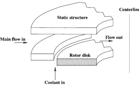
Centerline

Rotor disk

Rotor inlet

Exit diffuser

I

Rotor hub

hrust bearing

Rotor outlet

Figure 3-5: Schematic of the turbine rotor with a shaped exit diffuser

* Shaped diffuser are usually not robust to off design operation and there is still a large uncer-tainty in the operating point of the micro engine.

" Manufacturing of a curved shape is difficult in silicon (other materials may be used, but must

sustain high temperature).

For the reasons above, the concept was put aside to give more time to work on film cooling studies.

3.4

Comparison of Baseline and Improved Turbine Stage

This section focuses on the comparison of the baseline design with the improved design. Three types of information are presented.

The first is simply a view of the turbine stage geometry, along with views of the mesh used to simulate the flow with Fluent.

The second is a comparison of the expected operating point of the stages, at 100% design speed, with a balance of mass flow and pressure (but not heat flux or shaft work). It is very important

Metrics Baseline stage Improved stage Nozzle Guide Vane Baseline design (8 blades) Baseline + 4 degrees

NGV exit angle (degree) 74 77

Rotor inlet radius (mm) 2.5 2.96

Rotor exit radius (mm) 1.5 2

Number of rotor blades 15 20 (21 for fabrication)

Table 3.1: Summary of design characteristics of the baseline turbine design and the improved stage

to remember that the baseline turbine stage is coupled to the baseline compressor, whereas the improved turbine stage is coupled to the improved compressor rotor with hollow blades and open trailing edge.

Third performance maps of the turbines are presented. They provide data for comparison across an operating range.

3.4.1 Presentation of the Baseline and Improved Turbine Stage

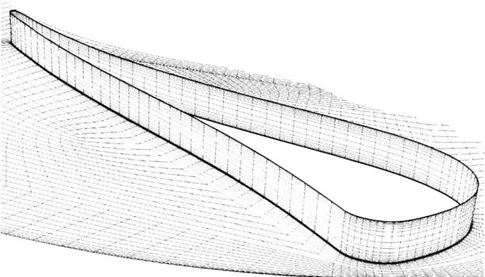
Figure 3-6 and 3-7 show example of the meshes which were used for the computations. The

number of nodes ranged from 100,000 to 150,000 to allow for fast computations and design studies. Boundary layers are resolved on end walls, on the blade surface (including the blade tip) and appear on the figures as dark and thick lines. The new stator is not included because the only difference from the baseline stator is a rotation of 4 degrees as detailed in table 3.1.

A top view of the baseline and improved turbine stage is presented in figure 3-8. The improved

rotor is quite different, because the leading edge radius has been moved upstream up to 2.96 mm and the trailing edge radius moved upstream to 2 mm to increase the exit area as explained in the first section of this chapter. All calculations on this rotor have been performed with a 20 blades rotor, but to limit unsteady interaction with the nozzle guide vane wake, a 21 blades rotor is proposed for fabrication. The impact of the addition of a blade has been assessed on another design (iteration 3) and has showed a 1.5% efficiency improvement and 0.5% mass flow decrease.