From an initial data to a global solution of the nonlinear Schrödinger equation: a building process

HAL Id: hal-01298989

https://hal.sorbonne-universite.fr/hal-01298989

HAL is a multi-disciplinary open access

archive for the deposit and dissemination of sci-entific research documents, whether they are pub-lished or not. The documents may come from teaching and research institutions in France or

L’archive ouverte pluridisciplinaire HAL, est destinée au dépôt et à la diffusion de documents scientifiques de niveau recherche, publiés ou non, émanant des établissements d’enseignement et de recherche français ou étrangers, des laboratoires

From an initial data to a global solution of the nonlinear

Schrödinger equation: a building process

Jean-Yves Chemin, Claire David

To cite this version:

Jean-Yves Chemin, Claire David. From an initial data to a global solution of the nonlinear Schrödinger equation: a building process. International Mathematics Research Notices, Oxford University Press (OUP), 2015, 2016 (8), pp.2376-2396. �10.1093/imrn/rnv199�. �hal-01298989�

From an initial data to a global solution of the nonlinear

Schrödinger equation: a building process

Jean-Yves Chemin, Claire David June 9, 2015

Université Pierre et Marie Curie-Paris 6 Laboratoire Jacques Louis Lions - UMR 7598

Boîte courrier 187, 4 place Jussieu, F-75252 Paris cedex 05, France

Abstract

The purpose of this work is to construct a continuous map from the homogeneous Besov space ˙B2,40 (R2) in the set G of initial data in ˙B2,40 (R2) which gives birth to global solution of

the mass critical non linear Schrödinger equation in the space L4_(R1+2_{). We use the fact that}

solutions of scale which are different enough almost do not interact; the main point is that we determine a condition about the size of the scale which depends continuously on the data.

1

Introduction

We consider in the space R2 _{the non linear Schrödinger equation of the type}

(GN LSm) {

i∂tu + ∆u = P3(u, u)

u_|t=0 = u0(x) (1)

where P3 is a homogeneous polynomial of order 3 in z and z. Let us observe that if we define uλ(t, x) =

λu(λ2t, λx) for a solution of (GN LSm) then uλ is also a solution. As we work in R2, the L2 norm, which represents the total mass, is invariant under this scaling transformation. This family of equations is thus called "mass critical".

As done for instance in [4], Strichartz estimate for the Schrödinger equation claims that for any couples (pj, qj)

2 p_j+

2

q_j = 1 and (pj, qj)̸= (2, ∞) =⇒ ∥u∥Lp1(I;Lq1(R2)). ∥u(I −_)∥

L2_(R2₎+∥i∂_t+ ∆u∥

Lp′2(I;Lq′2(R2₎₎.

(2) It is now classical to prove, with a fixed point argument, that Equation (GN LSm) is locally well posed for initial data in L2(R2), and globally well posed for small initial data in L2(R2). More precisely, we have the following theorem (see for instance [4]).

Theorem 1.1. Let u0 be an initial data in L2(R2). Then a positive time T exists such that there is

a unique solution to (GN LSm) in L4([0, T ]× R2). Moreover, a positive constant c0 exists such that,

if ∥u0∥L2_(R2₎ is less than or equal to c₀, the solution is global and belongs to L4(R1+2) and

∫

R1+2|u(t, x)|

4_{dxdt. ∥u}

0∥4_L2_(R2₎. (3)

Let us mention that some important particular cases of (GN LSm) have been intensively studied: the case when P3(u, u) =|u|2u, called defocusing case and the case when P3(u, u) =−|u|2u called the

focusing case. In the defocusing case, B. Dodson proves in [8] that for any initial data in L2(R2), a unique global solution exists in L4(R1+2) ; he proved in [9] that it was also the case in the focusing case when the mass of the initial data was less than the mass of the ground state. In the works [12] and [13], refined blow phenomena are described for initial data closed to the ground state.

In the present work, we proved general results far away from using the refined structure of the focusing or defocusing case. As observed by P. Gérard in an unpublished work (see the text [15] by F. Planchon and references therein), it is possible to improve a little this result using Besov spaces. For technical reasons, we prefer to use a continuous version of the Littlewood-Paley theory. Let us consider a radial function φ in D(Rd\ {0}) such that

φ(ξ) = f (|ξ|) with ∫ _∞ 0 f (r−1)dr r = 1 and thus ∫ _∞ 0 φ(µ−1ξ)dµ µ = 1 because the measure µ−1dµ is invariant under dilatation. Let us define ∆µa def= F−1

(

φ(µ−1ξ)ba(ξ)). Now let us recall the definition of Besov spaces.

Definition 1.1. We define the Besov space as the space of tempered distributions such that ∥u∥_B˙s p,r(Rd) def = µs∥∆µu∥Lp Lr_(R+_;dµ µ) .

The space ˙B_2,40 (R2), bigger than L2(R2) = ˙B_2,20 (R2), has the same scaling. One has the follow-ing result [4].

Theorem 1.2. Let u0 be an initial data in ˙B02,4(R2). Then a positive time T exists such that there is

a unique solution to (GN LSm) in L4([0, T ]× R2). Moreover, a positive constant c0 exists such that,

if ∥u0∥_B˙0

2,4(R2) is less than or equal to c0, the solution is global and belongs to L

4_(R1+2_{) and} ∫ R1+2|u(t, x)| 4_{dxdt. ∥u} 0∥4_B˙0 2,4 . (4)

It is proved in [15], which moreover proves the global existence of weak solutions for small initial data in B_2,0_∞. Let us give some sketchy indications about the proof of this theorem. Using an improvement of Strichartz inequality (2) proved by J. Bourgain in [2], we get

∥eit∆_u

0∥L4_(R1+2₎. ∥u₀∥_B˙0

2,4(R2). (5)

Then it is possible to make a fixed point theorem in the space L4_{([0, T ]× R}2_{). Let us point out that}

if u is a solution to (GN LSm) in the space L4([0, T ]× R2) then w = u− eit∆u0 satisfies

(i∂tw + ∆w) = P3(u, u)∈ L

4

3([0, T ]× R2) and w

|t=0 = 0.

Strichartz estimate (2) with (p2, q2) = (4, 4) and (p1, q1) = (∞, 2) implies that u − eit∆u0 belongs to

the space L∞([0, T ]; L2(R2)).

Definition 1.2. Let us denote byG the set of all initial data in ˙B_2,40 (R2) such that a global solution of (GN LSm) exists in L4(R1+2).

It is classical that the set G is an open subset of ˙B_2,40 (R2). Indeed, if u0 belongs to G, and v0

to ˙B0

2,4(R2), one can search the solution associated with u0+ v0 under the form u + v, where u is the

solution associated with u0. Elementary computations lead to

i∂tv + ∆v = E(u, v) with E(u, v)(t, x) . |v(t, x)| (

|u(t, x)|2_{+|v(t, x)|}2)_.

Inequalities (5) and (2) allow to prove that if v0 is small enough in the norm ˙B02,4(R2), then fixed point

argument works in the space L4(R1+2) for v.

The purpose of this work is to prove the following theorem. Theorem 1.3. A continuous function F from ˙B0

2,4(R2) intoG, and a constant C0 exist, such that

As far as we know, there is no results of this type in the literature. The motivation of this result is to catch some informations about the setG in the spirit of the works [5] by J.-Y. Chemin and I. Gallagher or [7] by J.-Y. Chemin, I. Gallagher and P. Zhang is the context of homogeneous incompressible Navier-Stokes equation. Unfortunately, the method presented here does not give any relevant result in the Navier-Stokes equation because in this case, it can be checked that the function F of our theorem (as constructed here) takes its value in a small ball of the space BM O−1 and thus is a small data in the sense of H. Koch and D. Tataru’s theorem (see [10]).

Let us discuss the choice of the space ˙B_2,40 (R2). We treated the case of L2(R2) in [6]. The two cases are closed technically. In the present state of the art, the biggest Besov space for which the free solution of the Schrödinger equation belongs to L4(R1+2), is ˙B_2,40 (R2).

2

Structure of the proof

The idea is to make the function v small by multiplication, and then to copy, as many times as required, a dilatation of the (now small) function. Let us introduce, for p in [1,∞[, the following notation:

π_S(p)vdef= v ∥v∥Lp and π_SBv = v ∥v∥_B˙0 2,4 ·

The first step consists in the definition of a functionF on ˙B0_2,4(R2)×R₊⋆ ×R+, with values in ˙B2,40 (R2),

which make explicit the idea explained above.

Definition 2.1. Let us consider a smooth function χ defined onR+such that χ_[

0,1₄]= 0 and χ[3 4,+∞[

= 1. Let us defineF from ˙B0_2,4(R2)× R₊⋆ × R+ into ˙B2,40 (R2) as follows

F(v, Λ, λ) =

[λ]

∑ j=0

Λ−jv(Λ−j·)+ χ (λ− [λ]) Λ−[λ]−1v(Λ−[λ]−1·).

We can wonder why we use dilation and not an other group of transformations that preserves the set of solutions of the equation to construct our function F . Here the key point is the continuity of F which comes from forthcoming Lemma 2.3. We have no idea how to prove such a lemma in another case of group, in particular in the case of the group of translations. The main properties of F are described hereafter.

Proposition 2.1. The mapF is continuous from ˙B_2,40 (R2)× R₊⋆ × R+ into ˙B02,4(R2). Moreover, there

exists a positive constant C and a continuous function Λ0 from ]1, +∞[×S( ˙B02,4(R2)) into R+ such

that, for any v in ˙B_2,40 (R2) different from 0, we have Λ> Λ0(λ + 1, π_SBv) =⇒ 1 C(λ + 1)∥v∥ 4 ˙ B0 2,4(R2)6 ∥F(v, Λ, λ)∥ 4 ˙ B0 2,4(R2)6 C(λ + 1) ∥v∥ 4 ˙ B0 2,4(R2). (6)

This proposition means that functions, the scales of which are different enough, are, in some sense, "orthogonal" in the Besov space ˙B_2,40 (R2). The main point of the proposition is that the choice of the scales size can be made continuously with respect to the function v.

Proposition 2.2. Let Bc0 be the open centered ball, the radius c0 of which is given by Theorem 1.2. There exists a continuous function Λ1 from ]1,∞[×Bc0 into ]0, +∞[ such that for any v in Bc0,

Λ> Λ1(λ + 1 , v) =⇒ F(v, Λ, λ) ∈ G.

The proof of this proposition relies on the idea that two solutions of an evolution equations with scales that are different enough almost do not interact. The idea which is now currently used goes back to the works of H. Bahouri and P. Gérard (see [1]) and F. Merle and L. Vega (see [14]). Again, it is related to the fact that the choice of the size can be made continuously with respect to the function v.

These two propositions imply Theorem 1.3. Indeed, if C0 is the constant given by Theorem 1.2, we define F (v) def= { 1− χ ( 3∥v∥_B˙0 2,4(R2) c0 )} v + χ ( 3∥v∥_B˙0 2,4(R2) c0 ) F(c0πB_Sv, Λ(v),∥v∥4_B˙0 2,4(R2) ) with Λ(v) def= Λ0 ( ∥v∥4 ˙ B0 2,4(R2) + 1, πB_Sv)+ Λ1 ( ∥v∥4 ˙ B0 2,4(R2) + 1, c0π_SBv ) .

Let us explain why this function F fulfills the requirements of Theorem 1.3. First of all, Proposi-tions 2.1 and 2.2 implies that F is continuous as a composition of continuous funcProposi-tions. Moreover, if ∥v∥_B˙0

2,4(R2) is less than or equal to c0 4, then we have F ( c0πB_Sv, Λ(v),∥v∥4_B˙0 2,4(R2) ) = v and thus also F (v) = v. Then thanks to Theorem 1.2, F (v) = v belongs to G. If ∥v∥_B˙0

2,4(R2) is greater than c0 4, then χ (_3∥v∥ ˙ B0_2,4(R2) c0 ) = 1, F (v) =F(c0π_SBv, Λ(v),∥v∥4_B˙0 2,4(R2) ) = v ; Proposition 2.1 implies that∥F (v)∥_B˙0

2,4(R2) is equivalent to ∥v∥B˙2,40 (R2) and Proposition 2.2 implies that F (v) belongs to G.

The idea of the proof of Proposition 2.1 is elementary: we develop the quantity∥F(v, Λ, λ)∥4 ˙

B0 2,4(R2)

and we prove that the cross terms are small enough thanks to the following lemma.

Lemma 2.3. Let us denote byS(Lp(Rd)) the unit sphere of the Lebesgue space Lp(Rd). For any p in ]1, +∞[, there exists a continuous function Λp from ]0, 1[×S(Lp(Rd))× S(Lp

′

(Rd_{)) such that for any} couple (f, g) of (Lp(Rd)\ {0})×(Lp′(Rd)\ {0}), one has

Λ> Λp(ε, π_S(p)f, π_S(p′)g)=⇒  ∫ Rd f (x)Λ− d p′_g(Λ−1_{x) dx} 6 ε∥f∥L p_(Rd₎∥g∥_Lp′_(Rd₎.

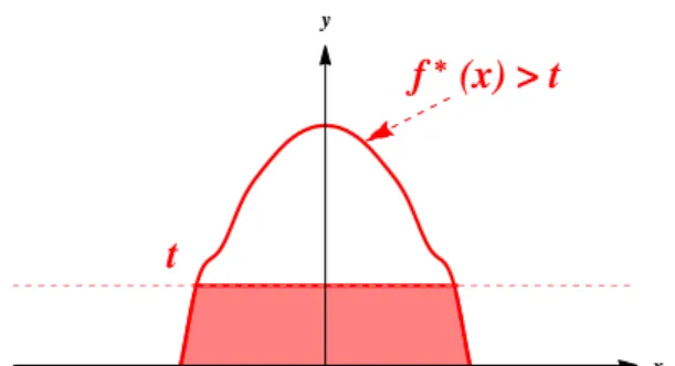
If one does not take continuity into account, the property is a very classical one: it is enough to approach, up to ε, the functions π_S(p)f and π(p_S′)g respectively in Lp _{and L}p′_{, by ring-supported} functions. Then, one chooses Λ large enough such that the integral of the truncated functions is 0. The question is: can the choice of the cut off be made continuously with respect to the functions? The answer is no, as shown by the following picture:

f (x) > t

t

Μ

(t)

x y

Figure 1: The graph of a non-negative function and measurable function f

If the function is radial and non increasing, it becomes possible. The use of the non-increasing reordering enables one to prove Lemma 2.3.

f

_{(x) > t}

t

x y

Figure 2: The graph of the rearrangement f⋆

Section 3 is, first, devoted to brief recalls on the definition and main properties of the symmetric non-increasing rearrangement. One proves, then, Lemma 2.3, which enables one to continuously truncate the rearrangements. Once it is done, one can prove Proposition 2.1.

Section 4 concentrates on the proof of Proposition 2.2, where Lemma 2.3 plays a major role re-garding continuity.

Section 5 is devoted to the proof of basic results on the non-increasing reordering which are collected here for the reader’s convenience.

3

Non-increasing reordering and almost-orthogonality

To begin with, let us work in the spaceRd_{. Let us, first, recall basic notations, that we will require} later on. For any measurable function f , we set

(f > t)def= {x∈ Rd/ f (x) > t} and (f 6 t)def= {x∈ Rd/ f (x)6 t}.

Let us consider a non-negative function and measurable function f : Rd → R, which vanishes at infinity, in the sense that, for any strictly positive real number t, the set (|f| > t) is of finite measure. Definition 3.1. Let A be a measurable set of Rd, the Lebesgue measure of which is finite. A⋆ denotes the open centered ball whose measure is the same of the one of A. Let us consider a real-valued, measurable function f , defined on Rd, which vanishes at infinity, in the sense that, for any strictly positive real number t, the set (|f| > t) is of finite measure. The symmetric non-increasing rearrangement of f is the measurable and non negative function f⋆_{, defined on [0, +∞[ by}

f⋆(x) = ∫ +∞

0

1(|f|>t)⋆(x) dt .

More detailed information can be found, for instance, in [11] and [18]. One can already notice that f⋆ =|f|⋆, and that the function f⋆ is a radially symmetric and non-increasing one, in the sense that f⋆_{(x) = f}⋆_{(y) if|x| = |y|, and f}⋆_{(x)> f}⋆_{(y) if|x| 6 |y|.}

We will require the non-increasing reordering properties described hereafter.

Proposition 3.1. Let us consider two real-valued, measurable functions f and g, defined onRd_{, which} vanishes at infinity. For any strictly positive number s,

( f (s·))⋆ = f⋆(s·), (7) ∫ Rd f (x)g(x)dx 6 ∫ Rd f⋆(x)g⋆(x)dx and (8) ∫ Rd f⋆(x)1_(g⋆_6s)(x)dx 6 ∫ Rd f (x)1_(g6s)(x)dx . (9) If, moreover, f and g belong to the space Lp, it is also the case of f⋆ and g⋆; in addition,

For the convenience of the reader, this proposition is proved in Section 5.

Proof of Lemma 2.3 Thanks to inequalities (7) and (8), one is led to find an upper bound to   ∫ Rd f (x)Λ− d p′_g(Λ−1_x)dx 6 I Λ def = ∫ Rd f⋆(x)Λ− d p′_g⋆_(Λ−1_{x)dx .}

As explained in the introduction, this means truncating the functions f⋆ and g⋆ in rings, which can be done using the following lemma.

Lemma 3.2. For any p in [1,∞[, there exists a continuous function R0 from ]0, 1[×S(Lp) to R+ such

that, for any f inS(Lp),

∥ϕR0(ε,f )f

⋆_∥

Lp = ε with ϕR(x)def= 1− 1_{{R−16|x|6R}}(x).

Proof. Let us first prove that, for any positive valued function h, radially symmetric, non-increasing, the Lp norm of which is equal to 1, and for any real number ε in ]0, 1[, there exists a unique R(ε, h)

such that _∫

Rd

ϕR(ε,h)(x)hp(x)dx = ε . From the dominated convergence theorem, the function

ρh(R)def= ∫

Rd

ϕR(x)hp(x)dx

is continuous and non-increasing on [1,∞[. Moreover : ρh(1) =∥h∥p_Lp = 1, and ρh(+∞) = 0. Let us denote by R_h the maximum of numbers R satisfying ρh(R) = 1. The function ρh is decreasing on the interval [R_h,∞[. Thus, there exists a unique Rh such that ρh(Rh) = εp. Applying this property to the function h = f⋆ enables one to define the function R0.

In order to prove the continuity of R0, let us consider a sequence (εn, fn) of ]0, 1[×S(Lp), which

converges towards (ε, f ) in ]0, 1[×S(Lp). It is enough to prove that any convergent subsequence con-verges towards R0(ε, f ). Let us denote by R∞the limit of a convergent subsequence of R0(εn, fn). For

sake of simplicity, extraction will not be distinguished. The triangle inequality leads to ∥ϕR0(εn,fn⋆)f ⋆ n∥Lp− ∥f⋆− f_n⋆∥_Lp6 ∥ϕR 0(εn,fn)f ⋆_∥ Lp 6 ∥ϕR 0(εn,fn)f ⋆ n∥Lp+∥f⋆− f_n⋆∥_Lp. By definition of R0, εn− ∥f⋆− fn⋆∥Lp 6 ∥ϕR 0(εn,fn)f ⋆_∥ Lp 6 εn+∥f⋆− f_n⋆∥_Lp.

Since the symmetric non-increasing rearrangement is 1−lipschtizian on the Lebesgue spaces Lp, one has

εn− ∥f − fn∥Lp 6 ∥ϕR

0(εn,fn)f ⋆_∥

Lp 6 εn+∥f − f_n∥_Lp. (10) The Lebesgue theorem implies then that:

lim

n→+∞ ϕR0(εn,fn)f ⋆

Lp =∥ϕR∞f⋆∥Lp.

By passing through the limit in (10), we obtain∥ϕR∞f⋆∥Lp_(Rd₎ = ε, which, by definition of R0, leads

to R_∞= R0(ε, f ). Then, the function R0 is a continuous one. The lemma is proved.

Conclusion of the proof of Lemma 2.3 One can estimate IΛ. Thanks to the identities

f⋆ = ϕ_{R0(ε,f )}f⋆+1 1 R0(ε,f)6|x|6R0(ε,f )f ⋆ _{and g}⋆ _{= ϕ} R0(ε,g)g ⋆₊₁ 1 R0(ε,g)6|x|6R0(ε,g)g ⋆_,

we have IΛ 6 ∫ Rd ( ϕR0(ε,f )f ⋆)_{(x) Λ}−p′d_g⋆ (_x Λ ) dx + ∫ Rd ( 1 1 R0(ε,f)6|x|6R0(ε,f )f ⋆)_{(x) Λ}−p′d(_ϕ R0(ε,g)g ⋆) ( x Λ ) dx + ∫ Rd ( 1 1 R0(ε,f)6|x|6R0(ε,f )f ⋆)_{(x) Λ}−_p′d (₁ 1 R0(ε,g)6|x|6R0(ε,g)g ⋆) ( x Λ ) dx 6 ∥ϕR0(ε0,f )f ⋆_∥ Lp∥g∥ Lp′ +∥f⋆∥Lp∥ϕ_R 0(ε,g)g ⋆_∥ Lp′ + ∫ Rd ( 1 1 R0(ε,f)6|x|6R0(ε,f )f ⋆)_{(x) Λ}−p′d (1 ₁ R0(ε,g)6|x|6R0(ε,g)g ⋆) ( x Λ ) dx. As∥f∥Lp=∥f⋆∥_Lp =∥g∥ Lp′ =∥g⋆∥_Lp′ = 1, this leads to IΛ 6 2ε + ∫ Rd ( 1 1 R0(ε,f )6|x|6R0(ε,f )f ⋆)_{(x) Λ}−p′d (1 ₁ R0(ε,g)6|x|6R0(ε,g)g ⋆) ( x Λ ) dx 6 2ε + ∫ Rd1 1 R0(ε,f)6|x|6R0(ε,f )(x)1 Λ R0(ε,g)6|x|6ΛR0(ε,g)(x) f ⋆_(x)Λ−p′d_g⋆ (_x Λ ) dx . Let us notice that if

Λ> 2R0(ε, f ) R0(ε, g) (11) then { x∈ Rd, 1 R0(ε, f ) 6 |x| 6 R0 (ε, f ) } ∩{x∈ Rd, Λ R0(ε, g) 6 |x| 6 ΛR0 (ε, g) } =∅. Thus, provided the condition (11) is satisfied, one has IΛ(f, g)6 2ε. For (f, g) in S(Lp)× S(Lp

′ ), let us define Λp(ε, f, g) def = 2R0 (_ε 2, f ) R0 (_ε 2, g ) . This function is suitable and Lemma 2.3 is thus proved.

Proof of Proposition 2.1 A basic expansion and the use of the scaling invariance lead to  ∥F(v, Λ, λ)∥4 ˙ B0 2,4 − ( ([λ] + 1) + (χ(λ− [λ]))4)∥v∥4_B˙0 2,4(R2)   . Ev,Λ,λ where Ev,Λ,λ def = ∫ _∞ 0 ∑ (j1,j2,j3,j4)∈ eJ ∆µ(Λ−j1_v(Λ−j1·)) L2 ∆µ(Λ−j2v(Λ−j2·)) _L2 × ∆µ(Λ−j3v(Λ−j3·)) _L2 ∆µ(Λ−j4v(Λ−j4·)) _L2 dµ µ with e J def= {0, . . . , [λ] + 1}4\{(j, j, j, j) , j ∈ {0, . . . , [λ] + 1}}. As we have ∆µ(Λ−jv(Λ−j·)) = Λ−j(∆µΛjv)(Λ−j·), one gets, due to the scaling of the L2 norm, that

E(v, Λ, λ) = ∫ _∞ 0 ∑ (j1,j2,j3,j4)∈ eJ ∆_µΛj1v _L2 ∆_µΛj2v _L2 ∆_µΛj3v _L2 ∆_µΛj4v _L2 dµ µ ·

Without any loss of generality, we can assume that j2 is smaller than j1 in the above integral. Hölder

inequality, for the measure dµ

µ , and the scaling invariance of this same measure, imply that ∫ _∞ 0 ∆_µΛj1v _L2 ∆µΛj2v _L2 ∆µΛj3v _L2 ∆µΛj4v _L2 dµ µ 6 ∥v∥2 ˙ B2,40 (R2) (∫ _∞ 0 _∆µv 2 L2 ∆_µΛ−(j1−j2)v 2 L2 dµ µ )1 2 ·

One deduces that: E(v, Λ, λ) . ([λ] + 1)3_∥v∥2 ˙ B0 2,4(R2) [λ]+1_∑ j=0 (∫ _∞ 0 ∆µv 2_L2 ∆µΛ−jv 2 L2 dµ µ )1 2 ·

The problem is reduced to the study of an integral of the form ∫ _∞

0

f (µ)g(Λ−1µ)dµ µ · with f and g in L2(]0,∞[; µ−1dµ). We define

e

f (µ)def= 1_[0,∞[(µ)f (µ) µ12

·

Let us now write that _{∫ ∞}

0 f (µ)g(Λ−1µ)dµ µ = ∫ R e f (µ)Λ−12eg(Λ−1µ) dµ .

Let us apply Lemma 2.3 with d = 1, p = 2 and let us choose ε = C([λ] + 1)−4; this gives Inequality (6). In order to prove the entire proposition, let us concentrate on the continuity ofF which comes mostly from the following lemma.

Lemma 3.3. The map

D { _˙

B_2,40 (R2)× R⋆₊ −→ ˙B_2,40 (R2) (v, δ) 7−→ δ−1v(δ−1·) is a continuous one.

Proof. It is worth noting that this map is an isometry in the sense that ∥D(v, δ)∥_B˙0

2,4 =∥v∥B˙02,4.

For any (v0, δ0) and (v, δ) belonging to ˙B2,40 (R2)× R⋆+,

∥D(v, δ) − D(v0, δ0)∥_B˙0 2,4(R2) 6 δ−1(v− v0)(δ−1·) _B˙0 2,4(R2)+ δ−1v0(δ−1·) − δ₀−1v0(δ₀−1·) _B˙0 2,4(R2) 6 ∥v − v0∥_B˙0 2,4(R2)+ v0− δ δ−10 v0(δ δ0−1·) _B˙0 2,4(R2) .

Let us then consider a strictly positive real number ε. There exists a function v0,ε ofD(R2) such that

∥v0− v0,ε∥_B˙0

2,4(R2)6 ε 4· This yields then, for any strictly positive real number δ,

v0− δ−1v0(δ−1·) _B˙0 2,4(R2) 6 ∥v0− v0,ε∥B˙ 0 2,4(R2)+ v0,ε− δ−1v0,ε ( δ−1·) _B˙0 2,4(R2) + δ−1v0,ε(δ−1·) − δ−1v0(δ−1·) _B˙0 2,4(R2) 6 2 ∥v0− v0,ε∥_B˙0 2,4(R2)+ v0,ε− δ−1v0,ε(δ−1·) _B˙0 2,4(R2) 6 2ε 4+ C v0,ε− δ −1_v 0,ε(δ−1·) _L2_(R2₎. As lim δ→1

Conclusion of the proof of Proposition 2.1 The above lemma assures that the functionF is continuous on L2(R2)× R⋆₊ × (R+\ N⋆). In order to conclude the proof, let us observe that, for any positive integer k, ∀ λ ∈ ]−1 4+ k, k + 1 4 [ , F(v, Λ, λ) = k ∑ j=0 Λ−jv(Λ−j·) (12)

which, thanks to Lemma 3.3, ensures the continuity of the function F on ˙B_2,40 (R2)× R⋆₊× R+. If λ belongs to the interval ]− 1/4 + k, k[, then [λ] = k − 1, χ(λ − [λ]) = 1, and Identity (12) is satisfied. If, now, λ belongs to the interval [k, k + 1/4[, then [λ] = k, χ(λ− [λ]) = 0, and the identity (12) is, again, satisfied. Proposition 2.1 is then proved.

4

Almost-orthogonality and making of global solutions

We hereafter aim at proving Proposition 2.2. Classically, one searches the solution related toF(v, Λ, λ) under the form uapp+ R, where the approached solution uapp(t, x) is given by

uapp(t, x) def = [λ]+1_∑ j=0 Vj,Λ(t, x) with Vj,Λ(t, x) def = Λ−jN LS(v)(Λ−2 jt, Λ−jx) for j in{1, · · · , [λ]} and V_[λ]+1,Λ(t, x) def= Λ−([λ]+1)N LS(χ(λ− [λ])v)(Λ−2([λ]+1)t, Λ−([λ]+1)x). and where the term R has to be understood as an error one.

The idea is that if we choose the scaling parameter Λ large enough, then the error term R is small, due to the fact that solutions of very different scale almost do not interact. The point here is thus to prove that the choice of the size of the parameter Λ can be made continuously when the function v varies. In order to do so, let us write the equation satisfied by the error term R. One has

{ i ∂tR + ∆R = EeΛ+ Φ(R) R_|t=0 = 0 with | eEΛ(t, x)| . EΛ(t, x) def = ∑ 06j,k,ℓ6[λ]+1 (j,k,ℓ)̸=(j,j,j) |Vj,Λ(t, x)| |Vk,Λ(t, x)| |Vℓ,Λ(t, x)| and |Φ(R)(t, x)| . |R(t, x)|3_+|u app(t, x)|2|R(t, x)|.

Here Φ is a generic notation used to denote a function of R that will not be explicitly given, for the sake of simplicity.

Let us estimate∥EΛ∥

L43(R1+2₎. By definition of the functions Vj,Λ, we get using the Hölder inequality

in the space variable E_Λj,k,ℓ def= ∫ R1+2|V j,Λ(t, x)|43|V_k,Λ(t, x)| 4 3|V_ℓ,Λ(t, x)| 4 3dxdt 6 ∫ RΛ −2 (j+k+ℓ) 3 NLS(v)(Λ−2 jt,·) 4 3 L4_(R2₎ × NLS(v)(Λ−2 kt,·) 4 3 L4_(R2₎ NLS(v)(Λ−2 ℓt,·) 4 3 L4_(R2₎dt.

As (j, k, ℓ) is not of the type (j, j, j), we can assume up to a perturbation of indices that k is smaller than ℓ. Hölder inequality and then a change of variable imply that

E_Λj,k,ℓ 6 (∫ R NLS(v)(Λ −2 j_t,·) 4 L4_(R2₎Λ−2jdt )1 3 × (∫ R NLS(v)(Λ −2 k_t,·) 2 L4_(R2₎Λ−(ℓ−k) NLS(v)(Λ−2 ℓt,·) 2 L4_(R2₎Λ−2kdt )2 3 6 ∥N LS(v)∥43 L4_(R1+2₎ (∫ R NLS(v)(t,·) 2 L4_(R2₎Λ−(ℓ−k) NLS(v)(Λ−2(ℓ−k)t,·) 2 L4_(R2₎dt )2 3 .

Applying Lemma 2.3, with d = 1, p = 2, f = g =∥N LS(v)(t, ·)∥2_L4_(R2₎, one gets

Λ> ΛF(ε, v)def= Λ2 ( ε, π(2)_S ∥N LS(v)(t, ·)∥2_L4_(R2₎, π (2) S ∥N LS(v)(t, ·)∥2L4_(R2₎ ) =⇒ E_Λj,k,ℓ 6 ε23∥N LS(v)∥4 L4_(R1+2₎.

As the function v is assumed to be in the ball Bρ, we have∥N LS(v)∥L4_(R1+2₎ . ∥v∥_˙

B2,40 (R2). Moreover

the map _{

Bρ −→ L2(R)

v 7−→ ∥N LS(v)(t, ·)∥2_L4_(R2₎

is continuous. Thus the map (ε, v)7−→ ΛF(ε, v) is continuous from ]0,∞[×Bρinto ]0,∞[, and we have Λ> ΛF(ε, v) =⇒ E_Λj,k,ℓ . ε23∥v∥4_˙

B0 2,4(R2)

. (13)

By definition of EΛ and Eλj,k,ℓ, we have ∥EΛ∥ 4 3 L43(R1+2₎. ∑ 06j,k,ℓ6[λ]+1 (j,k,ℓ)̸=(j,j,j) E_λj,k,ℓ.

With (13) this leads to

Λ> ΛF(ε, v) =⇒ ∥EΛ∥ L43(R1+2₎6 Cε 1 2([λ] + 1) 9 4∥v∥3 ˙ B0 2,4(R2) . (14)

The estimate of∥uapp∥L4_(R1+2₎ follows the same lines. Indeed, let us write that

 ∥uapp∥4_L4_(R1+2₎− [λ] ∑ j=0 ∥Vj,Λ∥4_L4_(R1+2₎ 6 ∑ 06j1,j2,j3,j46[λ]+1 j1,j2,j3,j4̸=(j,j,j,j) ∫ R1+2|Vj1,Λ (t, x)| |Vj2,Λ(t, x)| |Vj3,Λ(t, x)| |Vj4,Λ(t, x)| dxdt.

Up to a permutation of indices, we can assume that j1̸= j2. Hölder inequalities and scaling invariance

lead to  ∥uapp∥4_L4_(R1+2₎− [λ]+1_∑ j=0 ∥Vj,Λ∥4_L4_(R1+2₎ . ([λ] + 1)3_∥v∥2 ˙ _R ([λ]+1_∑ ∫ ∥N LS(v)(t, ·)∥2 4 _R2 Λ−j∥N LS(v)(Λ−2jt,·)∥24 _R2 dt )1 2 .

Applying Lemma 2.3, with d = 1, p = 2 and f = g =∥N LS(v)(t, ·)∥2_L4_(R2₎ gives Λ> ΛF(ε, v) =⇒∥uapp∥4_L4_(R1+2₎− ([λ] + 1)∥N LS(v)∥4_L4_(R1+2₎ 6 C([λ] + 1)4ε 1 2∥v∥4 ˙ B0 2,4(R2) . One deduces, then

( ε6 1 4 ([λ] + 1)6 and Λ> ΛF(ε, v) ) =⇒ ∥uapp∥4L4_(R1+2₎6 2C([λ] + 1)∥v∥4_B˙0 2,4(R2) . (15) Let us admit for a while that, for any time T smaller than the maximal time of existence T⋆,

∥R∥L4_{([0,T ]×R}2₎6 C ( ∥EΛ∥ L43(R1+2₎+∥R∥ 2 L4_{([0,T ]×R}2₎ )

exp(∥uapp∥4_L4_(R1+2₎

)

. (16)

A positive real number η being given, let us introduce the time Tη as Tη def = sup { 06 T < T⋆/ ∫ T 0 ∥R(t, ·)∥4 L4_(R2₎dt6 η4 } .

If we prove that T = T⋆ _{then the maximal time of existence T}⋆ _{will be equal to +∞. Using} Inequality (16) we get that for any T smaller than Tη,

∥R∥L4_{([0,T ]×R}2₎ 6 C ( ∥EΛ∥ L43₍R1+2₎+ η 2) _exp(_C∥u app∥4L4_(R1+2₎ ) . Let us choose η and ε such that

η = 1 4 C exp ( −C∥uapp∥4L4_(R1+2₎ ) and ε = η 2 4 C4_{([λ] + 1)}92 ∥v∥6 ˙ B0 2,4(R2) exp(−4 C([λ] + 1)∥v∥4_B˙0 2,4(R2) ) .

Assertions (14), (15) and (16) lead to∥R∥_L4_{([0,T ]×R}2₎ 6

3

4. Thus, Tη = T

⋆ _{which leads to T}⋆ _{= +∞.} Our theorem is proved provided it is the case of inequality (16). Let us introduce the increasing sequence (Tm)06m6M+1 such that T0 = 0, TM +1= +∞, and

∀ m < M ,

∫ Tm+1 Tm

∥uapp(t)∥4_L4_(R2₎dt = ε4₀ and

∫ TM +1 TM

∥uapp(t)∥4_L4_(R2₎dt6 ε4₀ (17)

for some given positive real number ε0, which will be chosen small enough later on. Obviously, we have

M ε4₀ 6 ∫ TM 0 ∥uapp(t)∥4L4_(R2₎dt6 ∫ +∞ 0 ∥uapp(t)∥4L4_(R2₎dt6 (M + 1)ε4₀. (18)

Thus the number M of Tm such that Tm is finite is less than ε−40 ∥uapp∥4_L4_(R1+2₎. Let us set R(T )def= ∥R∥_L∞_{([0,T ];L}2_(R2₎₎+∥R∥_L4_{([0,T ]×R}2₎₎.

We are going to prove, by induction, that for any T smaller than min{Tm, T⋆}, one has R(T ) 6 Cm+1

0 ∥EΛ∥L4/3_(R1+2₎.

Let us now consider a time T smaller than min{Tm+1, T⋆}. Strichartz estimate to the interval [Tm, T ] gives ∥R∥L∞([Tm,T ];L2(R2))+∥R∥L4([Tm,T ]×R2))6 C ( ∥R(Tm)∥L2_(R2₎+∥E_Λ∥ L43(R1+2₎ +∥R∥3_L4_([T m,T ]×R2))+∥R∥L4([Tm,T ]×R2))∥uapp∥ 2 L4_([T m,Tm+1]×R2)) ) .

By definition of ε0, we get ∥R∥L∞([Tm,T ];L2)+∥R∥L4([Tm,T ]×R2)) 6 C ( ∥R(Tm)∥L2_(R2₎+∥E_Λ∥ L43(R1+2₎ +(η2+ ε2₀)∥R∥L4_([T m,T ]×R2) ) . If C(η2+ ε2₀)6 1/2, one obtains ∥R∥L∞([Tm,T ];L2)+∥R∥L4([Tm,T×R2)6 2C ( ∥R(Tm)∥L2_(R2₎+∥E_Λ∥ L43(R1+2₎ ) . With the choice C0= 2C + 1, the induction hypothesis immediately yields

R(T ) 6 (2C + 1)Cm+1

0 ∥EΛ∥_L43(R1+2₎

6 Cm+2

0 ∥EΛ∥

L43(R1+2₎.

By induction, we deduce that, for any T less than T⋆,we have R(T ) 6 C₀M +2∥EΛ∥

L43(R1+2₎. Using

Inequality (18), it turns out that

R(T ) 6 C∥EΛ∥_L4 3(R1+2₎exp ( C ∫ _∞ 0 ∥uapp(t)∥4L4_(R2₎dt )

which implies Inequality (16). Proposition 2.2 is proved.

5

Some non-increasing reordering properties

We hereafter aim at proving proposition 3.1. More information can be found in [11], [18]. We nonethe-less recall the main results useful to our study. Various proofs of those results can be found in the above references. In the following, we concentrate on positive-valued functions. We will frequently refer to the fact that, for any function h,

h(x) = ∫ _∞

0

1(h>t)(x)dt. (19)

To prove (7), let us note that (f (s·) > t) = s−1(f > t). Let Rt denote the radius such that the volume of (f > t) is the same as the one of the centered ball of radius Rt. Thus we have

1(f (s·)>t)⋆(x) =1B(0,s−1Rt)(x) =1(f >t)⋆(sx). One obtains inequality (7) by integration in t.

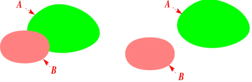
The proof of Inequality (8) relies on the following observation. Let A and B denote two sets ofRd of finite measure. If A⋆ and B⋆ are two centered balls, one has

This can be illustrated by the following drawing.

A

B

A

B

Figure 3: The sets A et B, with or without an intersection.

B*

A*

Figure 4: The centered balls A⋆ and B⋆.

Thanks to Fubini’s theorem, and to inequality (20), one has, from the definition of f⋆ and g⋆, ∫ Rd f⋆(x)g⋆(x)dx = ∫ Rd (∫ ∞ 0 1(f >t)⋆(x)dt )(∫ ∞ 0 1(g>s)⋆(x)ds ) dx = ∫ _∞ 0 ∫ _∞ 0 meas((f > t)⋆∩ (g > s)⋆)dtds. By applying (20) in the above relation, one gets:

∫ Rd f⋆(x)g⋆(x)dx> ∫ _∞ 0 ∫ _∞ 0 meas((f > t)∩ (g > s))dtds. If we apply then (19), we obtain:

∫ Rd f⋆(x)g⋆(x)dx > ∫ _∞ 0 ∫ _∞ 0 ∫ Rd1(f >t) (x)1(g>s)(x)dtdsdx > ∫ Rd (∫ ∞ 0 1(f >t)(x)dt )(∫ ∞ 0 1(g>s)(x)ds ) dx > ∫ Rd f (x)g(x) dx which ensures the required inequality.

The proof of Inequality (9) is a very close one. According to (19) and Fubini’s theorem, we get ∫ Rd f (x)1(g6s)(x)dx = ∫ Rd ∫ _∞ 0 1(f >t)(x)1(g6s)(x)dxdt = ∫ _∞ 0 meas((f > t)∩ (g 6 s))dt. (21)

As1_{(f >t)}1_(g6s) =1_{(f >t)}− 1_{(f >t)}1_(g>s), an integration leads to:

meas((f > t)∩ (g 6 s))= meas(f > t)− meas((f > t)∩ (g > s)). By applying (20) to the sets (f > t) and (g > s), one deduces

meas((f > t)∩ (g 6 s)) > meas((f > t)⋆)− meas((f > t)⋆∩ (g > s)⋆) > meas(f > t)⋆− meas((f⋆> t)∩ (g⋆> s)) > meas((f > t)⋆∩ (g⋆6 s)).

Using it in inequality (21) enables one to write, thanks to Fubini’s theorem, that ∫ Rd f (x)1(g6s)(x)dx > ∫ _∞ 0 ∫ Rd1(f >t) ⋆(x)1_(g⋆_6s)(x)dxdt > ∫ Rd f⋆(x)1(g⋆_6s)(x)dx which is Inequality (9).

To prove the equality of the Lp norms, let us note that, according to Fubini’s theorem, for any positive valued function h, and any p in [1,∞[, one has

∥h∥p Lp = p ∫ Rd ∫ _∞ 0 1(h>t)(x)tp−1dtdx = p ∫ _∞ 0 meas(h > t)tp−1dt .

By definition of ⋆ operation on sets, (f > t) and (f⋆ > t) are of same measure. The above formula ensures immediately the equality of the Lp norms.

The fact that the⋆ process is 1-lipschitzian on Lp(Rd) comes from the more general following result. Lemma 5.1. Let J denote a convex function from R to R+ such that J (0) = 0. If f and g are two positive-valued functions, then

∫ Rd J (f⋆(x)− g⋆(x)) dx6 ∫ Rd J (f (x)− g(x)) dx .

Proof. Let us write

J = J++ J− with J+

def

= 1_R+J and J₋ def= 1_R−_\{0}J.

The two functions J+ and J− are convex, and positive valued. One proves the inequality for J+, the

proof for J₋ being strictly analogous. Let h1 and h2 denote two non negative functions. One has

J+(h1(x)− h2(x)) = ∫ h1(x) h2(x) J₊′ (h1(x)− s) ds = ∫ +∞ h2(x) J₊′ (h1(x)− s) 1(h26s)(x) ds. (22)

If H is an increasing function on R+, its derivative in the sense of distributions is a non negative measure (which we denote by dH) and which satisfies

H(y− s) = ∫ _∞

0

Thanks to Fubini’s theorem, we deduce that, for any set of functions (h1, h2), ∫ Rd H(h1(x)− s)1(h26s)(x)dx = ∫ _∞ 0 (∫ Rd1(h1>s+t) (x)1(h26s)(x)dx ) dH(t). (23)

By applying this formula with (h1, h2) = (f⋆, g⋆), in conjunction with Inequality (9), one obtains,

thanks to the positivity of the measure dH(t), ∫ Rd H(f⋆(x)− s)1(g⋆_6s)(x)dx = ∫ Rd_×[0,∞[1(f ⋆_>s+t)(x)1_(g⋆_6s)(x)dxdH(t) 6 ∫ _∞ 0 (∫ Rd1(f >s+t) (x)1_(g6s)(x)dx ) dH(t).

If, now, we apply Formula (23) with the set of functions (f, g), we get ∫ Rd H(f⋆(x)− s)1(g⋆_6s)(x)dx6 ∫ Rd H(f (x)− s)1(g6s)(x)dx.

By applying this inequality with H = J₊′ , it ensures the required result, thanks to Formula (22).

Acknowledgment

The authors would like to thank Patrick Gérard, Fabrice Planchon, and the anonymous referee, for their judicious remarks and advices, which helped improving the original work.

References

[1] H. Bahouri and P. Gérard, High frequency approximation of solutions to critical nonlinear wave equations, American Journal of Math, 121, 1999, pages 131-175.

[2] J. Bourgain, Refinements of Strichartz’ inequality and applications to 2D-NLS with critical non-linearity, International Mathematical Research Notices, 5, 1998, pages 253-283.

[3] N. Burq, Explosion pour l’équation de Schrödinger au régime du "log-log", (d’après Merle-Raphael), Séminaire Bourbaki 2005/06), Astérisque 311, 2007, pages 33-53.

[4] T. Cazenave and F. Weissler, Some remarks on the nonlinear Schrödinger equation in the crit-ical case, Nonlinear Semigroups, Partial Differential Equations and Attractors Lecture Notes in Mathematics, 1394, Berlin, 1989, pages 18-29.

[5] J.-Y. Chemin and I. Gallagher, Wellposedness and stability results for the Navier-Stokes equations inR3_{, Annales de l’Institut Henri Poincaré, Analyse Non Linéaire, 26, 2009, pages 599–624.}

[6] J.-Y. Chemin, C. David, Sur la construction de grandes solutions pour des équations de Schrödinger de type "masse critique", to appear in Séminaire Équations aux Dérivées Partielles, École polytechnique, Palaiseau.

[7] J.-Y. Chemin, I. Gallagher and P. Zhang, Sums of large global solutions to the incompressible Navier-Stokes equations, Journal für reine und angewandte Mathematik, 681, 2013, pages 65-82. [8] B. Dodson, Global well-posedness and scattering for the defocusing, L2-critical, nonlinear

Schrödinger equation when d = 2, 2010, arXiv :1006.1375.

[9] B. Dodson, Global well-posedness and scattering for the mass critical nonlinear Schrödinger equa-tion with mass below the mass of the ground state, arXiv :1104.1114, 2011.

[10] H. Koch and D. Tataru: Well-posedness for the Navier-Stokes equations, Advances in Mathematics, 157, 2001, pages 22–35.

[11] E. Lieb and M. Loss, Analysis, Graduate Studies in Mathematics, 14 (American Mathematical Society, Providence, RI, 1997).

[12] F. Merle and P. Raphaël, On universality of blow up profile for L2 critical nonlinear Schrödinger equation, Inventiones Mathematicae, 156, 2004, pages 565-672.

[13] F. Merle, P. Raphaël, J. Szeftel, The instablility of Bourgain-Wang solutions for L2 critical NSL, American Jouranl of Mathematics, 135, 2013 pages 967-1017.

[14] F. Merle and L. Vega, Compactness at blow-up time for L2 solutions of the critical nonlinear Schrödinger equation in 2D, International Mathematical Research Notices, 1998, pages 399-425. [15] F. Planchon, Dispersive estimates and the 2D Cubic NLS equation, Journal d’Analyse

Mathéma-tique, 86, 2002, pages 319-334.

[16] F. Planchon, On the Cauchy problem in Besov spaces for a non-linear Schrödinger equation, Communicatons in Contemptary Mathematics, 2, 2000, pages 243-254.

[17] F. Planchon, Existence globale et scattering pour les solutions de masse finie de l’équation de Schrödinger cubique en dimension 2, Séminaire Bourbaki, 63eme` année, 2010-2011, n◦ 1042. [18] G. Pólya and G. Szegó, Isoperimetric inequalities in Mathematical Physics, Annals of Mathematics