L1-PCA signal subspace identification for non-sphered data under the ICA model

HAL Id: hal-01719134

https://hal.archives-ouvertes.fr/hal-01719134

Submitted on 1 Feb 2019

HAL is a multi-disciplinary open access

archive for the deposit and dissemination of

sci-entific research documents, whether they are

pub-lished or not. The documents may come from

teaching and research institutions in France or

abroad, or from public or private research centers.

L’archive ouverte pluridisciplinaire HAL, est

destinée au dépôt et à la diffusion de documents

scientifiques de niveau recherche, publiés ou non,

émanant des établissements d’enseignement et de

recherche français ou étrangers, des laboratoires

publics ou privés.

L1-PCA signal subspace identification for non-sphered

data under the ICA model

Rubén Martín-Clemente, Vicente Zarzoso

To cite this version:

Rubén Martín-Clemente, Vicente Zarzoso. L1-PCA signal subspace identification for non-sphered

data under the ICA model. Proc. CAMSAP-2017, 7th IEEE International Workshop on

Compu-tational Advances in Multi-Sensor Adaptive Processing, Dec 2017, Curaçao, Netherlands Antilles.

�hal-01719134�

L1-PCA Signal Subspace Identification for

Non-sphered Data Under the ICA Model

Rub´en Mart´ın-Clemente

Department of Signal Theory and Communications University of Seville, Spain

[email protected]

Vicente Zarzoso

Universit´e Nice Cˆote d’Azur, CNRS I3S Laboratory, Sophia Antipolis, France

[email protected]

Abstract—Principal component analysis (PCA) is an ubiquitous data compression and feature extraction technique in signal processing and machine learning. As compared with the classical L2-norm PCA, its L1-norm version offers increased robustness to outliers that are usually present in faulty data. Recently, L1-PCA was shown to perform source recovery when the observed data follow an independent component analysis (ICA) model. However, proof of this result requires the data to be sphered, i.e., to be preprocessed to constrain their covariance matrix to be the identity. The present contribution extends this result by relaxing the sphering assumption and allowing the data to have arbitrary covariance matrix. We prove that L1-PCA is indeed able to identify the mixing matrix columns associated with the strongest independent sources, thus performing signal subspace identification with improved robustness to outliers. Numerical experiments illustrate and confirm the theoretical findings.

I. INTRODUCTION

Principal Component Analysis (PCA) is probably the most popular multivariate data analysis technique [4], as it consti-tutes the basis for a variety of dimensionality reduction and noise filtering approaches. Multivariate data can be considered as vectors in a high-dimensional vector space, say Rp_{. The}

primary goal of PCA, as defined originally by Pearson, is to find the direction of the line that best fits the data in the p-dimensional space. In the traditional approach, this goal is obtained by maximizing the sum of the squares of the data projections onto the sought direction. Actually, several best fitting directions, or principal axes, can be computed by solving repeatedly the above optimization problem under the constraint that the nth principal axis has to be orthogonal to the previous (n 1) axes. The subspace V ⇢ Rp _spanned

by the orthogonal basis vectors pointing in the main principal directions is called the signal subspace, another fundamental concept in multivariate signal processing.

It is intuitive that the principal axes reveal much of the structure of the data. In the context of the processing of faulty data, PCA is mostly useful when the data of interest is concentrated around only a few principal axes, so that the dimension of the signal subspace V is much lower than p, whereas the noise is distributed isotropically through all Rp_{. In}

this case, a significant reduction of the noise, while preserving the information content of the original data, can be obtained by projecting the faulty data onto the signal subspace.

Recently, L1-norm PCA has been proposed in an attempt to increase robustness to outliers of classical PCA.

Experi-mentally, the L1-PCA approach has proven to be effective for restoration of faulty data in, e.g., the reconstruction of occluded images [6], [10], [11], as well as in pattern recog-nition and dimensionality reduction [1], [6]–[10], [13], [14], [16]–[18]. Although fast yet suboptimal algorithms for L1-PCA exist [5], [6], one of the most attractive features of this approach is that it can be also performed by optimal algorithms with guaranteed global convergence, as recently shown in [10]. The link between L1-PCA and independent component analysis (ICA), another popular multivariate data processing technique [3], [15], is carried out in [12], thus opening the possibility to perform ICA using globally optimal algorithms for L1-PCA. L1-PCA is shown to extract the independent sources under the ICA model in the case where the data are sphered, i.e., they have been whitened to present an identity covariance matrix. The present contribution extends this result by relaxing the assumption that the data be sphered, which defines a more general framework. A theoretical analysis supported by experimental results shows that L1-PCA is able to identify the dominant signal subspace under the ICA model, thus enabling source recovery via beamforming in a further processing stage.

II. PROBLEMFORMULATION

Let us suppose that we observe N samples {x1, x2, . . . , xN} of a p-dimensional zero-mean random

vector x, which can be arranged into the (p ⇥ N) matrix X = [x1, . . . , xN].

Let w 2 Rp_{, kwk}

2 = 1, define a projection direction. As

mentioned above, the goal of classical PCA is to find the random variable y = wT_{xwith the largest empirical variance.}

The first principal component vector solves the following problem: max kwk2=1 N X n=1 (wTxn)2

or, in matrix form:

max

kwk2=1

wTX ₂. (1) Though mathematically appealing, the L2-norm is rather sensitive to impulsive noise or outliers since squaring the

projections overemphasizes the effects of far-off data points, which is a serious drawback.

To increase the robustness of PCA when processing faulty data, we can try to eliminate the outliers from the data or, alternatively, replace the L2-norm cost function by a more robust criterion. The following L1-norm based variant of traditional PCA is proposed in [6]:

max kwk2=1 wT_X 1 (2) where kyk1 = PN

n=1|yi| represents the sum of the absolute

entries of vector y = wT_{X. The above two PCA criteria}

are generally not equivalent, even when the data contain no outliers. A key problem is to determine under which conditions the solutions of (1) and (2) are the same, or at least similar, in the absence of outliers. When the data are sphered, i.e., the covariance matrix Rx = _N1XXT equals the identity matrix,

it follows that wT_X

2 =kwk2 and therefore no principal

axis can be defined or identified according to (1). This is no surprising as sphering is often performed by classical PCA, so that the information that the L2 criterion can extract from sphered data is somewhat exhausted. By contrast, L1-PCA can yield interesting directions even for sphered data. A generative model that can provide useful insights is the case where each data point xi is made up of the linear superposition

xi = q

X

j=1

ajsij (3)

where sij represents the degree to which aj 2 Rp is present

in observation xi and q is the actual dimension of the data.

The assumption that coefficients sij are mutually independent

for different values of j is physically plausible in many real-world problems, and gives rise to the independent component analysis (ICA) model [3]. The solutions of L1-PCA under the ICA model when p = q and the data are sphered are analyzed in depth in [12], showing that projections associated with independent components are locally stable stationary points of the L1-PCA criterion.

The remaining of this paper explores the extension of this result to the more general case of non-sphered data, where Rx 6= I, and proves that L1-PCA yields principal directions

in a similar sense to L2-PCA but with the benefit of increased robustness to outliers.

III. THEORETICALANALYSIS

We conduct a preliminary study for the case q = 2, implying that the data points can be described by only two independent components. This case is simple enough to allow a theoretical analysis, while still retaining the important features of the problem. Results are stated without proof for lack of space. A. General Analysis for q = 2

We start by adopting a distributional viewpoint so that, according to model (3), the observed data vector x can be expressed as

x = a1s1+ a2s2= As (4)

with A = [a1, a2] and s = [s1, s2]T. Components s1 and s2

represent zero-mean, mutually statistically independent ran-dom variables, which are also assumed to have unit variance. If this is not the case, the power of the variables can always be incorporated into the length of the vectors ai without loss

of generality.

Given a projection unit-norm vector w, the projected data are defined by y = wT_{x = g}

1s1+ g2s2, where gi= wTai.

Denoting by aji the jth entry of ai, we can also write

gi= p

X

j=1

wjaji.

Observe that, assuming ergodicity conditions, the L1-norm criterion in (2) becomes (up to an irrelevant scale factor) proportional to E{|y|} for large enough sample size:

kyk1 !

N!+1N E{|y|}

where y = wT_{X. For this reason, instead of (2), let us}

consider here the equivalent problem max

w E{|y|} subject to kwk2= 1

whose Lagrangian is given by

L(w, ) =1₂E{|y|} + (kwk2

2 1) (5)

where is the Lagrange multiplier. Differentiating with respect to the components of w by the chain rule, and using some formulas in [12], it can be proven that

@_L @wn = 2 X i=1 aniGi+ 2 wn where Gi= Z 1 1 sfi(s)Fj ✓ gi gj s ◆ ds (6)

with i, j 2 {1, 2}, i 6= j,. Symbols fi(·) and Fj(·) denote

the probability density function and the distribution function, respectively, of sj. This equation can be rewritten in matrix

form as

@_L

@w = Ab + 2 w

where b = [G1,G2]T. Finally, the stationary points of the

criterion must verify: @L

@w = 0) Ab = 2 w. (7) This equation is difficult to solve because b depends nonlin-early on w through g in (6). Hence, rather than searching for a general solution, we will consider a simple yet significant particular problem for now.

B. Particular Case: Data Clustered Around 1D Subspace Now let us focus on the important situation where the data appear approximately clustered around a one-dimensional subspace, a straight line. Without loss of generality, we assume that this line is in the direction of a1, the case of a2 being

treated in a totally analogous manner. A necessary condition for the observed data clustering is that ka1k2 ka2k2

under the unit-variance source assumption. Vector a1 defines

a principal axis in the sense of the dominant signal subspace, while the term a2s2 is interpreted here as a small amount of

added noise defining a noise subspace. We are going to study whether L1-PCA is able to identify the signal subspace. This is tantamount to verifying whether

w⇡ ± a1 ka1k2

(8) is a solution to (7). Since, by definition,

g = wTA_{⇡ ±}h1, aT1a2/ka1k2

i

we can assume that g2

g1 ' 0. Then, the following

Maclaurin-based approximation of (6) holds for i = 2: G2⇡ Z 1 1 sf2(s)  F1(0) s f1(0) g2 g1 ds = f1(0) g2 g1

where we have exploited the assumption that s2has zero mean

and unit variance. Clearly, g2

g1 ' 0 implies G2' 0. Substituting

G2= 0in (7), we readily arrive at (8): this proves that a1 is a

stationary point of the L1-norm criterion. We know check its stability.

C. Local Stability Analysis

Let Lw be the Hessian matrix associated to (5), Lw =

Fw+ Hw, where Hw= " @2 @wi@wj p X n=1 w2n # i,j i, j = 1, . . . , p

is the Lagrange multiplier and Fwis the Hessian of1₂E{|y|},

Fw def =  _@2 @wi@wj 1 2E{|y|} _i,j i, j = 1, . . . , p. Assuming the solution (8), it can be shown that

Lw= f1(0) ka1k2 a2aT2 ka1k2 ✓Z 1 0 sf1(s) ds ◆ I. Let v be any vector orthogonal to w. Geometry shows that

vTa2=⌥kvk2ka2k2sin(\a1a2)

where\a1a2 is the angle between a1 and a2. Then,

vT_L wv kvk2 2 = ka2k 2 2 ka1k2 sin2(\a1a2)f1(0) ka1k2 Z 1 0 sf1(s) ds.

When ka1k2 is greater enough than ka2k2, it follows that

vT_L

wv < 0. According to [2], this ensures that (8) maximizes

the criterion. Otherwise, if f1(0) R₀1sf1(s) ds, as in a

supergaussian distribution [12], then vT_L

wvmay be positive:

in this case, we have to minimize, not maximize, the L1-norm to recover a1.

According to this theoretical analysis, L1-PCA determines the signal subspace in a way similar to L2-PCA. This result, combined with the fact that L1-PCA is more robust against outliers than L2-PCA, provides additional support for the use of L1-PCA in the analysis of faulty data.

IV. NUMERICALEXPERIMENTS

Some computer experiments are carried out to support the validity and generality of the theoretical development of the previous section. For simplicity we will assume that p = q, i.e., the observations have the same dimensionality as the underlying independent components generating the data. A. Case q = 2

Let a1 = p↵₂[1, 1]T and a2 = 1₂[p3, 1]T. These vectors

make an angle of 45 and 30 , respectively, with the horizontal axis so that Rx = AAT 6= I. Assuming that

w ⇡ ± a1

ka1k2 as in (8), it follows that ka1k2 ka2k2, as

required, when ↵ ! 1. We generate N = 200 samples of the random variable x using model (4), where s1and s2are drawn

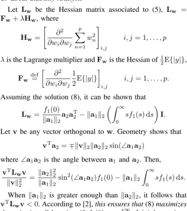
from independent zero-mean unit-variance uniform distribu-tions. L1-PCA is then applied on the data using the iterative algorithm presented in [6]. First, Figure 1 (top) shows vector a1 for ↵ = 1.5 (solid-line arrow), the vector wL1 obtained

by L1-PCA (bold solid line), the first principal component wL2 generated by traditional L2-PCA (dashed line) and the

scatter plot of the observations of x. In the figure, vectors a1, wL1 and wL2 have been shifted and scaled differently

for clarity. In this particular experiment, observe that L1-PCA estimates a1, the vector pointing in the main direction of the

data, better than L2-PCA: the angle between wL1 and a1

equals 3.2 , whereas the angle between wL2 and a1 is 6.3 .

Next, we repeat the experiment after adding several outliers to the same data. Results are shown in Figure 1 (bottom). As expected, the estimation is negatively affected by the presence of outliers: the angle between wL1and a1 now becomes 3.6 .

Yet L1-PCA proves more robust than L2-PCA, since the angle between wL2 and a1 is now equal to 12.5 .

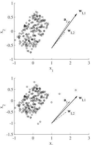
Figure 2 (left) shows the angle of vector wL1 determined

by L1-PCA with the horizontal axis as a function of ↵ after convergence of the L1-PCA algorithm. As ↵ increases, this angle tends to 45 so that wL1is parallel to a1as expected. On

the other hand, if ↵ tends to zero, the angle approaches 30 and wL1 coincides with a2, which is also consistent with our

analysis as a2 now becomes dominant. Finally, when ↵ = 1,

so that a1 and a2 have the same length, wL1 points in the

direction of the sum of both vectors. In Figure 2 (right), as in a previous experiment, data contain 5% of Gaussian outliers and therefore the figure also compares the robustness of L1-PCA and L2-L1-PCA.

B. Case q > 2

We now generate N = 500 independent samples of x = P7

x

x

x

x

Fig. 1. Scatter plot of a two-dimensional observation (p = 2) composed of two independent components (q = 2) and N = 200 samples. The independent component direction a1 is represented by a solid line arrow. The L1-PCA

solution wL1 (bold solid-line arrow) is aligned with the main axis of the

data, as predicted by our analysis. For the purposes of comparison, the L2-PCA solution wL2is also shown (dashed-line arrow). Vectors are not drawn

to scale. Top plot: No outliers. Bottom plot: 5% of outliers. Outliers are drawn at random from a normalized Gaussian distribution. It is apparent in this figure that L1-PCA is more robust to outliers than L2-PCA.

α

0.5 1 1.5 2 2.5 3

Angle with the horizontal

-30° 7.5° 45° L1-PCA L2-PCA α 0.5 1 1.5 2 2.5 3

Angle with the horizontal

-30° 7.5° 45°

L1-PCA L2-PCA

Fig. 2. Angle of L1-PCA solution wL1with the horizontal axis as a function

of the dominant axis magnitude ↵. As ↵ increases, the angle tends to 45 and wL1points in the direction of a1. As ↵ tends to zero, a2becomes dominant

and wL1points it its direction, at an angle of 30 . For comparison, the angle

between the L2-PCA solution and the horizontal axis is also shown in the dashed line. The curves represent the average of 100 independent experiments. Left plot: no outliers. Right plot: data contain 5% of outliers.

drawn from a standardized Gaussian distribution, except for a4, where the variance is set to 10, so that a4defines the main

axis of the data. The variables sj are zero-mean and uniformly

distributed. Figure 3 shows the angle of vector wL1recovered

by L1-PCA with each of the basis vectors ai, simply computed

as arccos⇣ |wT_a

i|

kwkkaik

⌘

, averaged over 100 independent Monte Carlo realizations. A confidence interval is also depicted: the total length of the vertical line equals twice the standard deviation of the angle. As expected, wL1 is more aligned

with a4 than with any other vector ai, i 6= 4. This result

demonstrates that the theoretical analysis of Sec. III can be generalized to the case of data with more than two dimensions (q > 2). For comparison, we also show the results obtained by L2-PCA.

Column number

Angle (degrees)

Fig. 3. Results with q = 7 random directions, where a4 has the strongest

magnitude, and N = 500 samples. Each pair of vertical lines represents the confidence intervals of the angles formed by L1-PCA vector wL1 (left

line) and the L2-PCA vector wL2(right line) with each data direction over

100 independent Monte Carlo realizations. L1-PCA succeeds in finding the principal direction naturally defined by the dominant axis a4. The results are

also similar to those obtained by applying L2-PCA.

V. CONCLUSIONS

This work has found a relationship between L1-PCA and the principal axes defining the dominant signal subspace when the data are not sphered. This result is consistent with the fact that the criterion seeks for projections with large amplitude. The dominant source subspace identified by L1-PCA proves more robust in the presence of outliers than classical L2-PCA. Further work should aim at the theoretical characterization of the influence of outliers and the extension of our analysis to more than two underlying dimensions.

ACKNOWLEDGMENTS

This work is partially funded by the Spanish Ministry of Economy and Competitiveness under project TEC2014-53103-P CMANS.

V. Zarzoso is a member of the Institut Universitaire de France.

REFERENCES

[1] J.P. Brooks, J.H. Dul´a, and E.L. Bone, “A pure L1-norm principal

com-ponent analysis”, Journal Computational Stat. Data Analysis, vol. 61, pp. 83–98, May 2013.

[2] E.K.P. Chong, and S. H. Zak, “An Introduction to Optimization”, John Wiley & Sons, Inc., 1996.

[3] P. Comon, and C. Jutten, eds. “Handbook of Blind Source Separation: Independent component analysis and applications”, Academic press, 2010.

[4] I.T. Jolliffe, “Principal Component Analysis”, Springer, 2nd ed., 2002. [5] S. Kundu, P. P. Markopoulos, and D. A. Pados, “Fast computation of the L1-principal component of real-valued data”, in Proceedings of 39th IEEE International Conference on Acoustics, Speech, and Signal Processing (ICASSP 2014), Florence, Italy, May 2014.

[6] N. Kwak, “Principal component analysis based on L1-norm maximiza-tion”, IEEE Transactions on Pattern Analysis and Machine Intelligence, vol. 30, pp. 1672–1680, Sept. 2008.

[7] N. Kwak and J. Oh, “Feature extraction for one-class classification prob-lems: enhancements to biased discriminant analysis”, Pattern Recogni-tion, vol. 42, pp. 17–26, Jan. 2009.

[8] X. Li, Y. Pang, and Y. Yuan, “L1-norm based 2DPCA”, IEEE Trans. on Systems, Man and Cybernetics, vol. 40, pp. 1170–1175, August 2009. [9] M. McCoy, and J. A. Tropp, “Two proposals for robust PCA using

semidefinite programming”, Electron. J. Stat., vol. 5, pp. 1123–1160, June 2011.

[10] P. P. Markopoulos, G. N. Karystinos, and D. A. Pados, “Optimal algorithms for L1-subspace signal processing”, IEEE Transactions on Signal Processing, vol. 62, no. 19, pp. 5046–5058, Oct. 2014. [11] P. P. Markopoulos, S. Kundu, S. Chamadia, and Dimitris A. Pados,

“Efficient L1-Norm Principal-Component Analysis via Bit Flipping”, IEEE Transactions on Signal Processing, vol. 65, no. 16, pp. 4252– 4264, Aug. 2017.

[12] R. Mart´ın-Clemente, V. Zarzoso, “On the link between L1-PCA and ICA”, IEEE Transactions on Pattern Analysis and Machine Intelligence, vol. 39, no. 3, pp. 515–527, March 2017.

[13] D. Meng, Q. Zhao, and Z. Xu, “Improve robustness of sparse PCA by L1 -norm maximization”, Pattern Recognition, vol. 45, pp. 487–497, Jan. 2012.

[14] Y. Pang, X. Li, and Y. Yuan, “Robust tensor analysis with L1-norm”, IEEE Trans. on Circuits and Systems for Video Technology, vol. 20, pp. 172–178, Feb. 2010.

[15] S. Roberts, and R. Everson, eds. “Independent Component Analysis: Principles and Practice”, Cambridge University Press, 2001.

[16] L. Yu, M. Zhang, and C. Ding, “An efficient algorithm for L1-norm principal component analysis”, Proc. IEEE ICASSP 2012, Kyoto, Japan, pp. 1377–1380, Mar. 2012.

[17] H. Wang, Q. Tang, and W. Zheng, “L1-norm-based common spatial patterns”, IEEE Trans. on Biomedical Engineering, vol. 59, pp. 653– 662, Mar. 2012.

[18] H. Wang, “Block principal component analysis with L1-norm for image analysis”, Pattern Recognition Letters, vol. 33, pp. 537-542, Apr. 2012.