HAL Id: hal-03053373
https://hal.archives-ouvertes.fr/hal-03053373
Submitted on 18 Dec 2020
HAL is a multi-disciplinary open access
archive for the deposit and dissemination of
sci-entific research documents, whether they are
pub-lished or not. The documents may come from
teaching and research institutions in France or
abroad, or from public or private research centers.
L’archive ouverte pluridisciplinaire HAL, est
destinée au dépôt et à la diffusion de documents
scientifiques de niveau recherche, publiés ou non,
émanant des établissements d’enseignement et de
recherche français ou étrangers, des laboratoires
publics ou privés.
simulations
Wesley de Nooijer, Qiong Zhang, Qiang Li, Qiang Zhang, Xiangyu Li,
Zhongshi Zhang, Chuncheng Guo, Kerim Nisancioglu, Alan Haywood, Julia
Tindall, et al.
To cite this version:
Wesley de Nooijer, Qiong Zhang, Qiang Li, Qiang Zhang, Xiangyu Li, et al.. Evaluation of Arctic
warming in mid-Pliocene climate simulations. Climate of the Past, European Geosciences Union
(EGU), 2020, 16 (6), pp.2325-2341. �10.5194/cp-16-2325-2020�. �hal-03053373�
https://doi.org/10.5194/cp-16-2325-2020 © Author(s) 2020. This work is distributed under the Creative Commons Attribution 4.0 License.
Evaluation of Arctic warming in mid-Pliocene
climate simulations
Wesley de Nooijer1, Qiong Zhang1, Qiang Li1, Qiang Zhang1, Xiangyu Li2,3, Zhongshi Zhang2,3,4, Chuncheng Guo3, Kerim H. Nisancioglu3, Alan M. Haywood5, Julia C. Tindall5, Stephen J. Hunter5, Harry J. Dowsett6,
Christian Stepanek7, Gerrit Lohmann7, Bette L. Otto-Bliesner8, Ran Feng9, Linda E. Sohl10,11, Mark A. Chandler10,11, Ning Tan12,13, Camille Contoux13, Gilles Ramstein13, Michiel L. J. Baatsen14, Anna S. von der Heydt14,15, Deepak Chandan16, W. Richard Peltier16, Ayako Abe-Ouchi17, Wing-Le Chan17, Youichi Kamae18, and Chris M. Brierley19
1Department of Physical Geography and Bolin Centre for Climate Research, Stockholm University, Stockholm, Sweden 2Institute of Atmospheric Physics, Chinese Academy of Sciences, Beijing, China
3NORCE Norwegian Research Centre, Bjerknes Centre for Climate Research, Bergen, Norway
4Department of Atmospheric Science, School of Environmental Studies, China University of Geosciences, Wuhan, China 5School of Earth and Environment, University of Leeds, Woodhouse Lane, Leeds, West Yorkshire, UK
6Florence Bascom Geoscience Center, U.S. Geological Survey, Reston, VA 20192, USA
7Alfred Wegener Institute – Helmholtz-Zentrum für Polar und Meeresforschung, Bremerhaven, Germany 8Palaeo and Polar Climate Division, National Center for Atmospheric Research, Boulder, CO 80305, USA 9Department of Geosciences, College of Liberal Arts and Sciences, University of Connecticut, CT 06269, USA 10Center for Climate Systems Research, Columbia University, New York, NY 10027, USA
11NASA Goddard Institute for Space Studies, New York, NY 10025, USA
12Key Laboratory of Cenozoic Geology and Environment, Institute of Geology and Geophysics, Chinese Academy of Sciences, Beijing, China
13Laboratoire des Sciences du Climat et de l’Environnement, LSCE/IPSL, CEA-CNRS-UVSQ, Universiteì Paris-Saclay, Gif-sur-Yvette, France
14Centre for Complex Systems Science, Utrecht University, Utrecht, The Netherlands 15Institute for Marine and Atmospheric research Utrecht (IMAU), Department of Physics, Utrecht University, Utrecht, The Netherlands
16Department of Physics, University of Toronto, Toronto, Ontario, Canada
17Centre for Earth Surface System Dynamics (CESD), Atmosphere and Ocean Research Institute (AORI), University of Tokyo, Tokyo, Japan
18Faculty of Life and Environmental Sciences, University of Tsukuba, Tsukuba, Japan 19Department of Geography, University College London, London, UK
Correspondence:Qiong Zhang (qiong.zhang@natgeo.su.se) Received: 1 May 2020 – Discussion started: 15 May 2020
Abstract. Palaeoclimate simulations improve our under-standing of the climate, inform us about the performance of climate models in a different climate scenario, and help to identify robust features of the climate system. Here, we analyse Arctic warming in an ensemble of 16 simula-tions of the mid-Pliocene Warm Period (mPWP), derived from the Pliocene Model Intercomparison Project Phase 2 (PlioMIP2).
The PlioMIP2 ensemble simulates Arctic (60–90◦N) an-nual mean surface air temperature (SAT) increases of 3.7 to 11.6◦C compared to the pre-industrial period, with a multi-model mean (MMM) increase of 7.2◦C. The Arctic warm-ing amplification ratio relative to global SAT anomalies in the ensemble ranges from 1.8 to 3.1 (MMM is 2.3). Sea ice extent anomalies range from −3.0 to −10.4 × 10⁶km2, with a MMM anomaly of −5.6 × 10⁶km2, which constitutes a de-crease of 53 % compared to the pre-industrial period. The majority (11 out of 16) of models simulate summer sea-ice-free conditions (≤ 1 × 10⁶km2) in their mPWP simula-tion. The ensemble tends to underestimate SAT in the Arc-tic when compared to available reconstructions, although the degree of underestimation varies strongly between the simu-lations. The simulations with the highest Arctic SAT anoma-lies tend to match the proxy dataset in its current form bet-ter. The ensemble shows some agreement with reconstruc-tions of sea ice, particularly with regard to seasonal sea ice. Large uncertainties limit the confidence that can be placed in the findings and the compatibility of the different proxy datasets. We show that while reducing uncertainties in the reconstructions could decrease the SAT data–model discord substantially, further improvements are likely to be found in enhanced boundary conditions or model physics. Lastly, we compare the Arctic warming in the mPWP to projections of future Arctic warming and find that the PlioMIP2 ensemble simulates greater Arctic amplification than CMIP5 future cli-mate simulations and an increase instead of a decrease in At-lantic Meridional Overturning Circulation (AMOC) strength compared to pre-industrial period. The results highlight the importance of slow feedbacks in equilibrium climate simula-tions, and that caution must be taken when using simulations of the mPWP as an analogue for future climate change.
1 Introduction
The simulation of past climates improves our understanding of the climate system, and it provides an opportunity for the evaluation of the performance of climate models beyond the range of present and recent climate variability (Braconnot et al., 2012; Harrison et al., 2014, 2015; Masson-Delmotte et al., 2013; Schmidt et al., 2014). Comparisons of palaeocli-mate simulations and palaeoenvironmental reconstructions have been carried out for several decades (Braconnot et al., 2007; Joussaume and Taylor, 1995) and show that while cli-mate models can reproduce the direction and large-scale
pat-terns of changes in climate, they tend to underestimate the magnitude of specific changes in regional climates (Bracon-not et al., 2012; Harrison et al., 2015). The comparison of palaeoclimate simulations with future projections has aided in the identification of robust features of the climate system which can help constrain future projections (Harrison et al., 2015; Schmidt et al., 2014), including in the Arctic (Yoshi-mori and Suzuki, 2019).
One such robust feature is the Arctic amplification of global temperature anomalies (Serreze and Barry, 2011). In-creased warming in the Arctic region compared to the global average is a common feature of both palaeoclimate and fu-ture climate simulations and is also present in the obser-vational record (Collins et al., 2013; Masson-Delmotte et al., 2013). Arctic warming has a distinct seasonal charac-ter, with the largest sea surface temperature (SST) and the smallest surface air temperature (SAT) anomalies occurring in the summer due to enhanced ocean heat uptake follow-ing sea ice melt (Serreze et al., 2009; Zheng et al., 2019). It is critical to correctly simulate Arctic amplification as it is shown that projected Arctic warming affects ice sheet sta-bility, global sea-level rise, and carbon cycle feedbacks (e.g. through permafrost melting; Masson-Delmotte et al., 2013). Several multi-model analyses that included palaeoclimate simulations and/or future projections found that changes in northern high-latitude temperatures scale (roughly) lin-early with changes in global temperatures (Bracegirdle and Stephenson, 2013; Harrison et al., 2015; Izumi et al., 2013; Masson-Delmotte et al., 2006; Miller et al., 2010; Schmidt et al., 2014; Winton, 2008).
Underestimation of Arctic SAT has been reported for sev-eral climates in the Palaeoclimate Modelling Intercompar-ison Project Phase 3 (PMIP3), including the mid-Pliocene Warm Period (Dowsett et al., 2012; Haywood et al., 2013a; Salzmann et al., 2013), Last Interglacial (LIG; Bakker et al., 2013; Lunt et al., 2013; Otto-Bliesner et al., 2013), and Eocene (Lunt et al., 2012a). PMIP4 simulations, however, of the LIG showed good agreement with SAT reconstructions in the Canadian Arctic, Greenland, and Scandinavia, while showing overestimations in other regions (Otto-Bliesner et al., 2020). PMIP4 simulations of the Eocene were also able to capture the polar amplification indicated by SAT proxies (Lunt et al., 2020).
In the present work, we analyse the simulated Arc-tic warming in a new ensemble of 16 simulations in the Pliocene Model Intercomparison Project Phase 2 (PlioMIP2) (Haywood et al., 2016). PlioMIP2 is designed to repre-sent a discrete time slice within the mid-Pliocene Warm Period (mPWP; 3.264–3.025 Ma; sometimes referred to as mid-Piacenzian Warm Period): Marine Isotope Stage (MIS) KM5c, 3.204–3.207 Ma (Dowsett et al., 2016, 2013; Hay-wood et al., 2013b, 2016). The mPWP is the most recent period in geological history with atmospheric CO2 concen-trations similar to the present, therefore providing great po-tential to learn about warm climate states. Additionally, the
KM5c time slice is characterized by a similar-to-modern or-bital forcing (Haywood et al., 2013b; Prescott et al., 2014). These factors give lessons learned from the mPWP and the KM5c time slice in particular, with potential relevance for fu-ture climate change (Burke et al., 2018; Tierney et al., 2019), and this is one of the guiding principles of PlioMIP (Hay-wood et al., 2016).
Palaeoenvironmental reconstructions show that the ele-vated CO2concentrations in the mPWP coincided with sub-stantial warming, which was particularly prominent in the Arctic (Brigham-Grette et al., 2013; Dowsett et al., 2012; Panitz et al., 2016; Salzmann et al., 2013; Haywood et al., 2020) discuss the large-scale outcomes of PlioMIP2 and ob-serve a global warming that is between the best estimates of predicted end-of-century global temperature change un-der the RCP6.0 (+2.2 ± 0.5◦C) and RCP8.5 (3.7 ± 0.5◦C; Collins et al., 2013) emission scenarios.
The dominant mechanism for global warming in mid-Pliocene simulations is through changes in radiative forc-ing followforc-ing increases in greenhouse gas concentrations (Chandan and Peltier, 2017; Hill et al., 2014; Hunter et al., 2019; Kamae et al., 2016; Lunt et al., 2012b; Stepanek et al., 2020; Tan et al., 2020). Polar warming is also dominated by changes in greenhouse gas emissivity (Hill et al., 2014; Tin-dall and Haywood, 2020). Apart from the changes in green-house gas concentrations, changes in boundary conditions that led to warming in previous simulations of the mPWP included the specified ice sheets, orography, and vegetation (Hill, 2015; Lunt et al., 2012b).
In PlioMIP1, the previous phase of this project, model simulations underestimated the strong Arctic warming that is inferred from proxy records was found (Dowsett et al., 2012; Haywood et al., 2013a; Salzmann et al., 2013). This data–model discord may have been caused by uncertainties in model physics, boundary conditions, or reconstructions (Haywood et al., 2013a).
Uncertainties in model physics include physical processes that are not incorporated in the models and uncertainties in model parameters. It was found that the inclusion of chemistry–climate feedbacks from vegetation and wildfire changes leads to substantial global warming (Unger and Yue, 2014), while excluding industrial pollutants, explicitly sim-ulating aerosol–cloud interactions (Feng et al., 2019), and decreasing atmospheric dust loading (Sagoo and Storelvmo, 2017) leads to increased Arctic warming in mPWP simu-lations. Similarly, in simulations of the Eocene, two mod-els that implemented modified aerosols had better skill than other models at representing polar amplification (Lunt et al., 2020). Changes in model parameters, such as the sea ice albedo parameter (Howell et al., 2016b), may provide fur-ther opportunities for increasing data–model agreement in the Arctic.
Several studies found changes in boundary conditions that could help resolve some of the data–model discord in the Arctic for PlioMIP1 simulations. The studied changes in
boundary conditions include changes in orbital forcing (Feng et al., 2017; Prescott et al., 2014; Salzmann et al., 2013), at-mospheric CO2 concentrations (Feng et al., 2017; Howell et al., 2016b; Salzmann et al., 2013), and palaeogeography and bathymetry (Brierley and Fedorov, 2016; Feng et al., 2017; Hill, 2015; Otto-Bliesner et al., 2017; Robinson et al., 2011). New in the experimental design of PlioMIP2 is a closed Bering Strait and Canadian Archipelago in the mPWP sim-ulation. The closure of these Arctic Ocean gateways has been shown to alter oceanic heat transport into the North At-lantic (Brierley and Fedorov, 2016; Feng et al., 2017; Otto-Bliesner et al., 2017). Additionally, the focus on a specific time slice within the mPWP allows for reduced uncertain-ties in reconstructions and boundary conditions, in particular with regards to orbital forcing. These changes have led to an improved data–model agreement for reconstructions of SST, particularly in the North Atlantic (Dowsett et al., 2019; Mc-Clymont et al., 2020; (Haywood et al., 2020). Multi-model mean (MMM) SST anomalies in the North Atlantic deviate less than 3◦C from reconstructed temperatures (Haywood et al., 2020).
In the following sections, we first evaluate the simulated Arctic (60–90◦N) temperatures and sea ice extents (SIEs) in the PlioMIP2 ensemble. We then perform a data–model com-parison for SAT and an evaluation of how uncertainties in the reconstructions may affect the outcomes of the data–model comparison. We then compare the simulated sea ice to recon-structions. Lastly, we investigate two climatic features of the mPWP, namely Arctic amplification and the Atlantic Merid-ional Overturning Circulation (AMOC), and compare these analyses to findings of future climate studies to investigate the extent to which the mPWP can be used as an analogue for future Arctic climate change.
2 Methods
2.1 Participating models
The simulations of the mPWP by 16 models participating in PlioMIP2 were used in this study. The models included in this study are listed in Table 1. A more detailed descrip-tion of each model’s informadescrip-tion and experiment setup can be found in Haywood et al. (2020). All model groups in-corporated the standardized set of boundary conditions from the PlioMIP2 experimental design in their simulations (Hay-wood et al., 2016).
For each simulation, the last 100 years of data are used for the analysis. Individual model results are calculated on the native grid of each model. MMM results are obtained af-ter regridding each model’s output to a 2◦×2◦ grid using bilinear interpolation. Using a non-weighted ensemble mean theoretically averages out biases in models, assuming models are independent, and errors are random (Knutti et al., 2010). Climate models can, however, generally not be assumed to be independent (Knutti et al., 2010; Tebaldi and Knutti, 2007),
Table 1.Models participating in PlioMIP2 used in this study.
Model name Institution PlioMIP2 reference CCSM4-NCAR National Center for Atmospheric
Research (NCAR)
Feng et al. (2020)
CCSM4-Utrecht IMAU, Utrecht University
CCSM4-UofT University of Toronto, Canada Chandan and Peltier (2017)
CESM1.2 NCAR Feng et al. (2020)
CESM2 NCAR Feng et al. (2020)
COSMOS Alfred Wegener Institute Samakinwa et al. (2020), Stepanek et al. (2020) EC-Earth 3.3 Stockholm University Q. Zhang et al. (2020) GISS–E2–1–G NASA/GISS Kelley et al. (2020) HadCM3 Hadley Centre for Climate Prediction and
Research/Met Office UK
Hunter et al. (2019)
IPSLCM5A Laboratoire des Sciences du Climat et de l’Environnement (LSCE)
Tan et al. (2020)
IPSLCM5A–2.1 LSCE Tan et al. (2020)
IPSL-CM6A–LR LSCE Lurton et al. (2020)
MIROC4m CCSR/NIES/FRCGC, Japan Chan and Abe-Ouchi (2020) MRI–CGCM2.3 Meteorological Research Institute Kamae et al. (2016) NorESM-L NORCE Norwegian Research Centre, Bjerknes
Centre for Climate Research, Bergen, Norway
Li et al. (2020)
NorESM1-F NORCE Norwegian Research Centre, Bjerknes Centre for Climate Research, Bergen, Norway
Li et al. (2020)
and this is especially true for the PlioMIP2 ensemble where many models have common origins (Table 1). The MMM re-sults will therefore likely be biased towards specific common errors within the models comprising the ensemble.
2.2 Data–model comparisons
To evaluate the ability of climate models to simulate mPWP Arctic warming, we first perform a comparison to SAT estimates from palaeobotanical reconstructions. The data– model comparison is performed using temperature anoma-lies, calculated by differencing the mPWP and the pre-industrial simulation, to avoid overestimations of agreement due to strong latitudinal effects on temperature (Haywood and Valdes, 2004).
Reconstructed mPWP SATs are taken from Feng et al. (2017), who updated and combined an earlier compilation made by Salzmann et al. (2013) (Table S1). Qualitative esti-mates of confidence levels for each reconstruction were made by Feng et al. (2017) and Salzmann et al. (2013). Only recon-structions that are located at or northward of 60◦N and for
which the temporal range covers the KM5c time slice are in-cluded in the data–model comparison. Three reconstructions from Ballantyne et al. (2010) at the same location (78.3◦N, −80.2◦E) were averaged to avoid oversampling that loca-tion. The uncertainties in the reconstructions were derived by Feng et al. (2017) and Salzmann et al. (2013) from relevant literature.
The data–model comparison will be a point-to-point com-parison of modelled and reconstructed temperatures esti-mated from palaeobotanical proxies, which initially does not take the uncertainties of the reconstructions (Table S1) into account. The potential influence of the uncertainties in re-constructions on the outcomes of the data–model compari-son will be investigated in a later section. The temporal range of the reconstructions is broad and certainly not resolved to the resolution of the KM5c time slice, unlike the dataset of SST estimates compiled by Foley and Dowsett (2019) used for PlioMIP2 SST data–model comparisons by Haywood et al. (2020) and McClymont et al. (2020). Prescott et al. (2014) found that peak warmth in the mPWP would be diachronous between different regions based on simulations with
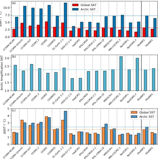
differ-Figure 1.Simulated global and Arctic (a) SAT anomalies (mPWP minus pre-industrial simulations), (b) Arctic amplification ratio of SAT, and (c) SST anomalies for each model and the MMMs. The horizontal lines represent PlioMIP2 MMM values.
ent configurations of orbital forcing. Orbital forcing is par-ticularly important in the high latitudes and for proxies that may record seasonal signatures (e.g. due to recording grow-ing season temperatures). As such, there may be significant biases in the dataset, as the temporal ranges of the proxies include periods with substantially different external forcing than during the KM5c time slice for which the simulations are run. Feng et al. (2017) investigated the effects of differ-ent orbital configurations, as well as elevated atmospheric CO2 concentrations (+50 ppm) and closed Arctic gateways in PlioMIP1 simulations, and found that they may change the outcomes of data–model comparisons in the northern high latitudes by 1–2◦C.
Further uncertainties arise due to bioclimatic ranges of fos-sil assemblages, errors in pre-industrial temperatures from the observational record, potential seasonal biases, and ad-ditional unquantifiable factors. Ultimately, the uncertainties constrain our ability to evaluate the Arctic warming in the PlioMIP2 simulations substantially. A more detailed descrip-tion of the uncertainties in the SAT estimates can be found in the work of Salzmann et al. (2013).
The reconstructed temperatures are differenced with peratures from the observational record to obtain proxy tem-perature anomalies. Observational-record temtem-peratures are obtained from the Berkeley Earth monthly land and ocean dataset (Rohde et al., 2013a, 2013b), and the average tem-perature in the 1870–1899 period was used.
Furthermore, the simulation of mPWP SIE will be eval-uated using three palaeoenvironmental reconstructions that indicate whether sea ice was perennial or seasonal at a spe-cific location. Darby (2008) infers that perennial sea ice was present at Lomonosov Ridge (87.5◦N, 138.3◦W) through-out the last 14 Myr based on estimates of drift rates of sea ice combined with inferred circum-Arctic sources of detri-tal mineral grains in sediments at this location. Knies et al. (2014) infer seasonal sea ice cover based on the abun-dance of the IP25biomarker, a lipid that is produced by cer-tain sea ice diatoms, which is similar to the modern summer minimum throughout the mid-Pliocene in sediments at two locations near the Fram Strait, of which one is chosen for this data–model comparison (80.2◦N, 6.4◦E). Similarly, Clotten et al. (2018) infer seasonal sea ice cover with occasional
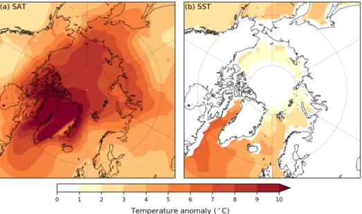
sea-Figure 2.MMM annual temperature anomalies in the Arctic: (a) SAT and (b) SST. At least 15 out of 16 models agree on the sign of change at each location.
ice-free conditions in the Iceland Sea (69.1◦N, −12.4◦E) be-tween 3.5 and 3.0 Ma using a multiproxy approach. As the sediment record studied by Clotten et al. (2018) included a peak in the abundance of the IP25 biomarker at 3.2 Ma, we infer seasonal sea ice cover during the KM5c time slice.
3 Arctic warming in the PlioMIP2 ensemble
3.1 Annual mean warming
The PlioMIP2 experiments show substantial increases in global annual mean SAT (ranging from 1.7 to 5.2◦C, with a MMM of 3.2◦C; Fig. 1a; Table S2) and SST (ranging from 0.8 to 3.9◦C, with a MMM of 2.0◦C; Fig. 1c; Table S2) in the mPWP, compared to pre-industrial period.
All models show a clear Arctic amplification, with an-nual mean SAT in the Arctic (60–90◦N) increasing by 3.7 to 11.6◦C (MMM of 7.2◦C; Fig. 1a). The magnitude of Arc-tic amplification, defined as the ratio between the ArcArc-tic and global SAT anomaly, ranges from 1.8 to 3.1, and the MMM shows an Arctic amplification factor of 2.3 (Fig. 1b). There is a large variation in the magnitude of the simulated Arctic SAT anomalies, with 5 out of 16 models, namely CCSM4-Utrecht, CCSM4-UoT, CESM1.2, CESM2, and EC-Earth 3.3, all simulating much stronger anomalies than the rest of the ensemble. This subset of the ensemble raises the MMM substantially, and this has to be taken into account when in-terpreting the MMM results. The MMM SAT anomaly for the PlioMIP2 ensemble excluding this subset of five models is 5.8◦C.
Annual mean SST in the Arctic increased by 1.3 to 4.6◦C (MMM of 2.4◦C; Fig. 1c). Furthermore, the five models that simulated the largest Arctic SAT anomalies also simulate the largest Arctic SST anomalies. Temperature anomalies in the
PlioMIP2 ensemble are similar but slightly higher than in the PlioMIP1 ensemble. A similar magnitude of Arctic amplifi-cation is simulated by the two ensemble means.
The greatest MMM SAT anomalies in the Arctic are found in the regions with reduced ice sheet extent on Greenland (Haywood et al., 2016), which generally show warming of over 10◦C and even up to 20◦C. Additionally, temperature anomalies of over 10◦C are simulated around the Baffin Bay. SAT anomalies of around 6–9◦C are simulated over most of the Arctic Ocean regions. SST anomalies in the Arctic are strongest in the Baffin Bay and the Labrador Sea, reaching up to 7◦C (Fig. 2b).
3.2 Seasonal warming
The distinct seasonality of Arctic amplification (Serreze et al., 2009; Zheng et al., 2019) can be used to identify mecha-nisms causing Arctic amplification. Figure 3 depicts the sea-sonality of Arctic warming for each model, with monthly SAT and SST anomalies normalized by the annual mean anomaly for that specific model.
The ensemble simulates a consistent peak in Arctic SST warming between July and September (Fig. 3b). This is con-sistent with the response that increased seasonal heat storage from incoming heat fluxes would have upon the reduction of SIE (Serreze et al., 2009; Zheng et al., 2019). Minimum SAT warming is expected in the summer because of the in-creased ocean heat uptake, while maximum SAT warming is expected in the autumn and winter following the release of this heat (Pithan and Mauritsen, 2014; Serreze et al., 2009; Yoshimori and Suzuki, 2019; Zheng et al., 2019). This is not simulated by all models, however (Fig. 3a). COSMOS, GISS-E2-1-G, IPSL-CM6A-LR, and MRI-CGCM2.3 all do
Figure 3.Ratio between the mean Arctic (a) SAT and (b) SST warming in a given month and the annual mean Arctic warming, for each model (and MMM) individually. Values of zero would imply no warming compared to pre-industrial period in a given month.
Figure 4.Mean annual SIE (106km2) for the pre-industrial and mPWP simulations. The horizontal lines represent PlioMIP2 MMM values.
show this autumn and winter amplification of annual mean SAT anomalies and decreased warming in the summer. De-creased summer warming is simulated by CCSM4-Utrecht, EC-Earth 3.3, and IPSLCM5A in combination with autumn amplification and by CESM2 and NorESM1-F in combina-tion with winter amplificacombina-tion. All other models in the en-semble do not show an autumn or winter amplification in combination with decreased summer warming, suggesting a more limited role of reductions in SIE underlying the sea-sonal cycle of Arctic SAT anomalies.
4 Sea ice analysis
4.1 Annual mean sea ice extent
The MMM of Arctic annual SIE (sea ice concentration ≥ 0.15) is 11.9 × 10⁶km2 for the pre-industrial simulations, and 5.6 × 10⁶km2(a 53 % decrease) for the mPWP simula-tions. The pre-industrial annual mean SIE ranges from 9.1 to 15.6 × 10⁶km2 in the ensemble, while the mPWP SIE ranges from 2.3 to 10.4 × 10⁶km2. The decrease in SIE be-tween individual simulations ranges from −3.0 × 10⁶km2 to −10.4 × 10⁶km2(Table S2). Interestingly, the PlioMIP1
MMM shows larger SIEs in both the pre-industrial and the mPWP simulations than any individual model in the PlioMIP2 ensemble (Fig. 4). The 53 % MMM decrease in SIE simulated by the PlioMIP2 ensemble is substantially greater than the 33 % MMM decrease in SIE simulated by the PlioMIP1 ensemble (Howell et al., 2016a).
4.2 Monthly mean sea ice extent
The seasonal cycle of SIE anomalies is depicted in Fig. 5a. Reductions in SIE are slightly greater in the autumn (September-November) compared to other seasons for the MMM. There is, however, no consistent response in the sea-sonal character of SIE anomalies in the PlioMIP2 ensemble. CCSM4-UoT, CESM2, IPSLCM5A, and IPSLCM5A-2.1 simulate the largest reductions in SIE in winter (December– February), while GISS-E2-1-G and HadCM3 simulate the largest SIE reductions in spring. The remaining 10 models simulate the greatest SIE anomalies in autumn.
A more consistent response is observed when comparing monthly mean mPWP SIEs and pre-industrial SIEs. For each model, the largest reductions in SIE in terms of percentages
Figure 5. (a) Monthly SIE anomalies relative to annual mean anomalies, warmer colours highlight in which months reductions in sea ice were largest. (b) Reduction in SIE (%) in the mPWP simulations compared to the pre-industrial monthly mean SIE for each month. Highlighted in bold italics in (b) are months with sea-ice-free conditions (SIE < 1 × 10⁶km2).
occur between August and October (Fig. 5b). This may be explained by the lesser amount of energy that is needed to melt a given percentage of the smaller SIE that is present in the summer compared to winter. A total of 11 out of 16 models simulate sea-ice-free conditions (SIE < 1 × 10⁶km2) in at least 1 month, while five models (GISS-E2-1-G, IP-SLCM5A, IPSLCM5A-2.1, MRI-CGCM2.3, and NorESM-L) do not (Fig. 5b). The NorESM1-F simulation simulates the smallest global mean warming (1.7◦C; Fig. 1a) resulting in Arctic sea-ice-free conditions.
4.3 Sea ice and Arctic warming
There is a strong anti-correlation between annual mean Arc-tic SAT and SIE anomalies (R = −0.79; Fig. 6a), as well as between SST and SIE anomalies (R = −0.79; Fig. 6b). These anti-correlations are stronger than those found for the PlioMIP1 ensemble (R = −0.76, R = −0.73, respectively; Howell et al., 2016a).
5 Data–model comparison surface air temperatures
5.1 Results
To evaluate the ability of the PlioMIP2 ensemble to simulate Arctic warming, we perform a data–model comparison with the available SAT reconstructions for the mPWP. The data– model comparison hints at a substantial mismatch between models and temperature reconstructions. Mean absolute de-viations (MAD) range from 5.0 to 11.2◦C (Table S3), with a MAD of 7.3◦C for the MMM. The median bias ranges from −2.0 to −13.1◦C, with a median bias of −8.2◦C for the MMM (Table S3). The PlioMIP2 MMM shows slightly improved agreement with the SAT reconstructions
compared to the PlioMIP1 MMM (MAD = 7.8◦C, median bias = −8.7◦C). Figure 7 depicts the deviation from recon-structions for the MMM. Underestimations range from −17 to −2.5◦C, while at two sites in the Canadian Archipelago (80◦N, 85◦W and 79.85◦N, 99.24◦W) the MMM overesti-mates the reconstructed temperatures (by 2.7 and 1.2◦C, re-spectively). It has to be noted, however, that SAT anomalies are underestimated at three other sites within the Canadian Archipelago. Given the resolution of global climate models and the close proximity of the sites, it may be impossible for simulations to match all five of these SAT estimates.
The deviation from reconstructions for each model and the PlioMIP2 and PlioMIP1 MMMs is represented by the box and whisker plots in Fig. 8. A consistent underesti-mation of the temperature estimates from SAT reconstruc-tions is present in the PlioMIP2 ensemble. CESM2 sim-ulates the smallest deviations from reconstructions in the ensemble, with a MAD of 5.0◦C and a median bias of −2◦C. The five models that simulated the highest Arctic SAT anomalies (CCSM4-Utrecht, CCSM4-UoT, CESM1.2, CESM2, and EC-Earth 3.3) simulate the lowest median bi-ases, indicating that the upper end of the range of simulated Arctic SAT anomalies in the PlioMIP2 ensemble tends to better match the proxy dataset in its current form. Future research into the underlying mechanisms for the increased Arctic warming in these 5 simulations, compared to the re-maining 11 simulations in the ensemble, may form a way to uncover factors that contribute to improved data–model agreement.
5.2 Uncertainties
Some of the data–model discord may be caused by uncertain-ties in the temperature estimates (Table S1; Salzmann et al.,
Figure 6.Correlations between annual mean SIE anomalies and (a) Arctic SAT anomalies and (b) Arctic SST anomalies. Depicted for both correlations are the correlation coefficient (R), the slope, and the probability value (p) that when the variables are not related, a statistical result equal to or greater than observed would occur.
Figure 7.Point-to-point comparison of MMM and reconstructed SAT. The size of SAT reconstructions is scaled by qualitatively as-sessed confidence levels (Salzmann et al., 2013). Data markers for reconstructions in close proximity of each other have been slightly shifted for improved visibility.
2013). To investigate how these uncertainties may have af-fected the outcomes of the data–model comparison, we con-struct a maximum uncertainty range. This range spans from the highest possible temperature within uncertainty and the lowest possible temperature within uncertainty. The uncer-tainties for the temperature estimates were taken from the compilation of mPWP Arctic SAT estimates from Feng et al. (2017) (Table S1).
Figure 8.Box and whisker plots depicting the distribution of biases (models minus reconstruction) with biases over (under) 0 represent-ing locations where models overestimated (underestimated) recon-structed temperatures. Boxes depict the interquartile ranges (IQRs) of the distribution, whiskers extend to the 2.5th and 97.5th per-centiles, the median is displayed by a horizontal line in the boxes, and outliers (outside of the 97.5th percentile) are shown by open circles outside of the whiskers. Given the sample size of 15 recon-structions, the two outer values are depicted as outliers using these definitions.
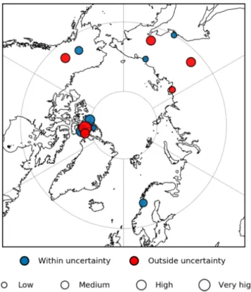
Figure 9 depicts the locations for which at least one model in the ensemble simulates a temperature within the maximum available uncertainty range of a reconstruction. For 6 out of the 12 reconstructions that included an uncertainty estimate, the models in the PlioMIP2 ensemble simulate temperatures that are within the uncertainty range (Fig. 9). Additionally, both overestimations and underestimations are present for the Magadan District reconstruction for which no uncertainty estimate is available (60◦N, 150.65◦E, Table S1), implying that the reconstruction falls within the range of simulated temperatures in the PlioMIP2 ensemble. For the remaining six reconstructions, including several which are assessed at high or very high confidence (Fig. 9), no model simulates temperatures within the uncertainty range.
Ultimately, when considering the full uncertainty ranges of the reconstructions, it becomes evident that solely reducing potential errors in SAT estimates would not fully resolve the
Figure 9.Blue circles highlight where at least one model in the ensemble simulates a temperature that falls within the uncertainty range of the reconstruction. The size of SAT reconstructions is scaled by qualitatively assessed confidence levels (Salzmann et al., 2013). Data markers for reconstructions in close proximity of each other have been slightly shifted for improved visibility.
data–model discord for several locations in the Arctic. It is thus likely that other sources of error contribute to the data– model discord, such as uncertainties in model physics (e.g. Feng et al., 2019; Howell et al., 2016b; Lunt et al., 2020; Sa-goo and Storelvmo, 2017; Unger and Yue, 2014) and bound-ary conditions (e.g. Brierley and Fedorov, 2016; Feng et al., 2017; Hill, 2015; Howell et al., 2016b; Otto-Bliesner et al., 2017; Prescott et al., 2014; Robinson et al., 2011; Salzmann et al., 2013). The focus on the KM5c time slice has helped re-solve some of the data–model discord that was present in the North Atlantic for SST (Haywood et al., 2020), and similar work for SAT reconstructions may thus be beneficial. How-ever, this may not always be possible given the lack of precise dating and chronologies available. It is at this moment un-clear whether the underestimation of Arctic SAT is specific to the mid-Pliocene, through uncertainties in reconstructions or boundary conditions, or an indicator of common errors in model physics.
6 Evaluation of sea ice
The limited availability of proxy evidence (three reconstruc-tions) severely limits our ability to evaluate the simulation of mPWP sea ice in PlioMIP2 simulations. Nevertheless, a
data–model comparison is still worthwhile, as the few re-constructions that are available may form an interesting out-of-sample test for the simulation of sea ice in the PlioMIP2 models.
Figure 10a depicts the number of models per grid box that simulate perennial sea ice. Six models simulate the in-ferred perennial sea ice (mean sea ice concentration ≥ 0.15 in each month) at Lomonosov Ridge (87.5◦N, 138.3◦W; Darby, 2008), while the remaining 10 simulate sea-ice-free conditions in at least 1 month per year at this site. The majority of the models simulate a maximum SIE that ex-tends, or nearly exex-tends, into the Fram Strait and Iceland Sea (Fig. 10b) in at least 1 month (in winter) per year (Fig. 10b), consistent with proxy evidence (Clotten et al., 2018; Knies et al., 2014).
The uncertainties in both the SAT and SIE reconstructions are large, and it may not be possible to match both datasets in their current forms. This would require increased Arc-tic annual terrestrial warming compared to the mean model (Sect. 5.1) as well as perennial sea in the summer and a large SIE in winter (extending at least into the Iceland Sea). Moreover, McClymont et al. (2020) found that the warmest model values in the PlioMIP2 ensemble tend to align best with North Atlantic SST reconstructions, further indicating that strong Arctic warming is required for data–model agree-ment. If there was no perennial sea ice in the mPWP like most models in the PlioMIP2 ensemble, the different proxy records may be more compatible, but this would be in dis-agreement with findings from Darby (2008). The CCSM4-Utrecht model, which simulated a relatively high Arctic SAT anomaly (10.5◦C; Fig. 1a) and low median bias (−4◦C) in the point-to-point SAT data–model comparison compared to the rest of the ensemble, simulates a maximum winter SIE that extends both into the Fram Strait and Iceland Sea. This highlights that models with higher Arctic SAT anomalies and better SAT data–model agreement can still match both sea-sonal sea ice proxies. Ultimately, more reconstructions of sea ice are needed for a more robust evaluation of mPWP sea ice and Arctic warming in general.
7 Comparison to future climates
Research into the mPWP is often motivated by a desire to understand future climate change (Burke et al., 2018; Hay-wood et al., 2016; Tierney et al., 2019). Here, we analyse how the mPWP may teach us about future Arctic warming by comparing two climatic features of the mPWP simula-tions to simulasimula-tions of future climate. The climatic features include Arctic amplification and a feature for which there is some proxy evidence available that may also aid in model evaluation: the AMOC.
Figure 10.Number of models simulating (a) annual mean perennial sea ice (sea ice concentration of ≥ 0.15) at any given location in the Arctic in the mPWP simulations and (b) monthly mean sea ice in any month of the year. Depicted squares represent the locations of the reconstructions and their respective colour the inferred mPWP sea ice conditions at that location.
Figure 11.(a) The relationship between global and Arctic (60–90◦N) temperature anomalies in the PlioMIP2 ensemble. The red trend line is constructed based on this relationship for the individual models. (b) The relationship between global and Arctic (here 67.5–90◦N, the definition used by Masson-Delmotte et al. (2013) and the area for which they listed data) for the MMMs of the two PlioMIP and the four CMIP5 future climate ensembles (2081–2100 average). The blue trend line highlights this relationship for the RCP MMMs.
7.1 Arctic amplification
A linear relationship between global and Arctic tempera-ture anomalies is present in the PlioMIP2 ensemble (R = 0.93, Fig. 11a). This is consistent with findings from multi-model analyses of other climates (Bracegirdle and Stephen-son, 2013; Harrison et al., 2015; Izumi et al., 2013; Masson-Delmotte et al., 2006; Miller et al., 2010; Schmidt et al., 2014; Winton, 2008) and indicates that global temperature anomalies are a good index for Arctic SAT anomalies in mPWP simulations.
For four ensembles of future climate simulations, from the previous phase of the Coupled Model Intercomparison Project (CMIP), CMIP5, data for MMM Arctic (defined there as 67.5–90◦N) temperature anomalies are available
(Masson-Delmotte et al., 2013; Table S4). The PlioMIP2 MMM shows global warming that falls between the RCP6.0 and RCP8.5 MMMs in terms of magnitude (Fig. 11b). Even though PlioMIP underestimates mPWP SAT reconstructions (Sect. 5.1), the simulations do simulate stronger Arctic tem-perature anomalies per degree of global warming compared to future climate ensembles (Fig. 11b). The future climate en-semble MMMs simulate end-of-century (2081–2100) aver-age Arctic (67.5–90◦N) amplification ratios that range from 2.2 to 2.4, while PlioMIP2 and PlioMIP1 simulate mean ra-tios of 2.8 and 2.7, respectively (Table S4).
The increased Arctic warming per degree of global warm-ing indicates that apart from warmwarm-ing through changes in at-mospheric CO2concentrations, which is the dominant
mech-anism for warming in both ensembles, different or additional mechanisms underly the simulated mPWP Arctic warming compared to the future climate simulations. The difference between the PlioMIP2 and future climate ensembles may be explained by slow responses to changes in forcings that fully manifest in equilibrium climate simulations, such as the response to reduced ice sheets, but not in transient, near-future climate simulations. Additional Arctic warming in the mPWP simulations may arise due to the changes in orog-raphy (Brierley and Fedorov, 2016; Feng et al., 2017; Hay-wood et al., 2016; Otto-Bliesner et al., 2017), ice sheets, and vegetation in the boundary conditions (Hill, 2015; Lunt et al., 2012b).
Using PlioMIP2 simulations for potential lessons about fu-ture warming may be improved by isolating the effects of the changes in orograph. Similar changes in ice sheets and vegetation may occur in future equilibrium warm climates, but the changes in orography are definitively non-analogous to future warming. Several groups isolated the effects of the changed orography on global warming in PlioMIP2 simu-lations and found that it contributes, respectively, around 23 % (IPSL6-CM6A-LR; Tan et al., 2020), 27 % (COS-MOS; Stepanek et al., 2020), and 41 % (CCSM4-UoT; Chan-dan and Peltier, 2018) to the annual mean global warming in the mPWP simulations. Furthermore, this warming was strongest in the high latitudes (Chandan and Peltier, 2018; Tan et al., 2020) indicating that the additional Arctic warm-ing in PlioMIP2 simulations, as compared to future climate simulations, are likely partially caused by changes in orogra-phy that are non-analogous with the modern-day orograorogra-phy. These findings highlight the caution that has to be taken when using palaeoclimate simulations as analogues for future cli-mate change.
7.2 Atlantic meridional overturning circulation
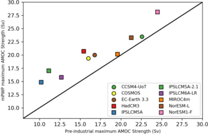
The AMOC, a major oceanic current transporting heat into the Arctic (Mahajan et al., 2011), is inferred to have been sig-nificantly stronger in the mPWP compared to pre-industrial values based on proxy evidence (Dowsett et al., 2009; Frank et al., 2002; Frenz et al., 2006; McKay et al., 2012; Rav-elo and Andreasen, 2000; Raymo et al., 1996). An analy-sis of AMOC changes in PlioMIP2 simulations shows that, indeed, the maximum AMOC strength increases: by 4 % to 53 % (Fig. 12; Table S2: Z. Zhang et al., 2020). The closure of the Arctic Ocean gateways, in particular the Bering Strait, likely contributed to the increase in AMOC strength (Brier-ley and Fedorov, 2016; Feng et al., 2017; Haywood et al., 2016; Otto-Bliesner et al., 2017).
Strengthening of the AMOC contrasts projections of fu-ture changes by CMIP5 models that predict a weakening of the AMOC over the 21st century, with best estimates ranging from 11 % to 34 % depending on the chosen future emission scenario (Collins et al., 2013). These opposing responses may help explain some of the additional Arctic warming that
Figure 12.Maximum pre-industrial and mPWP AMOC strength (Sv). The black line indicates equal pre-industrial and mPWP max-imum AMOC strength.
is observed in the PlioMIP2 ensemble compared to the future climate ensembles (Fig. 11b).
The strengthening of the AMOC in the PlioMIP2 en-semble is consistent with the additional 0.4◦C increase in SST warming in the Arctic (Fig. 1c) and the better data– model agreement in the North Atlantic that is observed for the PlioMIP2 MMM (Dowsett et al., 2019; Haywood et al., 2020; McClymont et al., 2020) compared to the PlioMIP1 MMM (Fig. 1c), which did not show any substantial changes in AMOC strength compared to pre-industrial values (Zhang et al., 2013).
8 Conclusions
The PlioMIP2 ensemble simulates substantial Arctic warm-ing and 11 out of 16 models simulate summer sea-ice-free conditions. Comparisons to reconstructions show, however, that the ensemble tends to underestimate the available re-constructions of SAT in the Arctic, although large differ-ences in the degree of underestimation exist between the sim-ulations. The models that simulate the largest Arctic SAT anomalies tend to match the reconstructions better, and inves-tigation into the mechanisms underlying the increased Arc-tic warming in these simulations may help uncover factors that could contribute to improved data–model agreement. We find that, while some of the SAT data–model discord may be resolved by reducing uncertainties in proxies, additional improvements are likely to be found in reducing uncertain-ties in boundary conditions or model physics. Furthermore, there is some agreement with reconstructions of sea ice in the ensemble, especially for seasonal sea ice. The limited availability of proxy evidence and the uncertainties associ-ated with them severely constrain the compatibility of the different proxy datasets and our ability to evaluate the Arctic warming in PlioMIP2. Increased proxy evidence of differ-ent climatic variables and additional sensitivity experimdiffer-ents,
among other goals, are needed for a more robust evaluation of Arctic warming in the mPWP. Lastly, we find differences in Arctic climate features between the PlioMIP2 ensemble and future climate ensembles that include the magnitude of Arctic amplification and changes in AMOC strength. These differences highlight that caution has to be taken when at-tempting to use simulations of the mPWP to learn about fu-ture climate change.
Data availability. The reconstructions used in this study are avail-able in the Supplement. The model data can be downloaded from PlioMIP2 data server located at the School of Earth and Environ-ment of the University of Leeds, an email can be sent to Alan Hay-wood (a.m.hayHay-wood@leeds.ac.uk) for access. At the time of publi-cation, the data from CESM2, EC-EARTH3.3, GISS-E2-1-G, IPSL-CM6A-LR, and NorESM1-F can be downloaded through CMIP Search Interface at https://esgf-node.llnl.gov/search/cmip6, last ac-cess: 17 November 2020; Department of Energy, 2020.
Supplement. The supplement related to this article is available online at: https://doi.org/10.5194/cp-16-2325-2020-supplement.
Author contributions. QZ and WdN designed the work. WdN did the analyses and wrote the manuscript under supervision from QZ. QL and QZ performed the simulations with EC-Earth3. XL and ZZ provided input on AMOC analysis. HJD provided the input on reconstructions. All the other co-authors provided the PlioMIP2 model data and commented on the manuscript.
Competing interests. The authors declare that they have no con-flict of interest.
Special issue statement. This article is part of the special issue “PlioMIP Phase 2: experimental design, implementation and scien-tific results”. It is not associated with a conference.
Acknowledgements. The EC-Earth3 simulations are performed on the Swedish National Infrastructure for Computing (SNIC) at the National Supercomputer Centre (NSC). COSMOS PlioMIP2 simulations have been conducted at the Computing and Data Cen-ter of the Alfred-Wegener-Institut Helmholtz-Zentrum für Polar und Meeresforschung on a NEC SX-ACE high-performance vec-tor computer. Gerrit Lohmann and Christian Stepanek acknowl-edge funding via the Alfred Wegener Institute’s research pro-gramme PACES2. Christian Stepanek acknowledges funding by the Helmholtz Climate Initiative REKLIM. Camille Contoux and Gilles Ramstein thank ANR HADOC ANR-17-CE31-0010; the authors were granted access to the HPC resources of TGCC un-der the allocations 2016-A0030107732, 2017-R0040110492, 2018-R0040110492 (gencmip6), and 2019-A0050102212 (gen2212) pro-vided by GENCI. The IPSL-CM6 team of the IPSL Climate Mod-elling Centre (https://cmc.ipsl.fr, last access: 17 November 2020)
is acknowledged for having developed, tested, evaluated, and tuned the IPSL climate model, as well as having performed and published the CMIP6 experiments. Wing-Le Chan and Ayako Abe-Ouchi ac-knowledge funding from JSPS KAKENHI grant 17H06104 and MEXT KAKENHI grant 17H06323 and also acknowledge JAM-STEC for the use of the Earth Simulator supercomputer. The PRISM4 reconstruction and boundary conditions used in PlioMIP2 were funded by the U.S. Geological Survey Climate and Land Use Change Research and Development Program. Any use of trade, firm, or product names is for descriptive purposes only and does not imply endorsement by the U.S. Government.
Financial support. This research has been supported by the Vetenskapsrådet (grant nos. 2013-06476, 2017-04232).
The article processing charges for this open-access publication were covered by Stockholm University.
Review statement. This paper was edited by Alessio Rovere and reviewed by two anonymous referees.
References
Bakker, P., Stone, E. J., Charbit, S., Gröger, M., Krebs-Kanzow, U., Ritz, S. P., Varma, V., Khon, V., Lunt, D. J., Mikolajewicz, U., Prange, M., Renssen, H., Schneider, B., and Schulz, M.: Last interglacial temperature evolution – a model inter-comparison, Clim. Past, 9, 605–619, https://doi.org/10.5194/cp-9-605-2013, 2013.
Ballantyne, A. P., Greenwood, D. R., Damsté, J. S. S., Csank, A. Z., Eberle, J. J., and Rybczynski, N.: Significantly warmer Arctic surface temperatures during the Pliocene indi-cated by multiple independent proxies, Geology, 38, 603–606, https://doi.org/10.1130/G30815.1, 2010.
Bracegirdle, T. J. and Stephenson, D. B.: On the Robust-ness of Emergent Constraints Used in Multimodel Climate Change Projections of Arctic Warming, J. Clim., 26, 669–678, https://doi.org/10.1175/JCLI-D-12-00537.1, 2013.
Braconnot, P., Otto-Bliesner, B., Harrison, S., Joussaume, S., Pe-terchmitt, J.-Y., Abe-Ouchi, A., Crucifix, M., Driesschaert, E., Fichefet, Th., Hewitt, C. D., Kageyama, M., Kitoh, A., Laîné, A., Loutre, M.-F., Marti, O., Merkel, U., Ramstein, G., Valdes, P., Weber, S. L., Yu, Y., and Zhao, Y.: Results of PMIP2 coupled simulations of the Mid-Holocene and Last Glacial Maximum – Part 1: experiments and large-scale features, Clim. Past, 3, 261– 277, https://doi.org/10.5194/cp-3-261-2007, 2007.
Braconnot, P., Harrison, S. P., Kageyama, M., Bartlein, P. J., Masson-Delmotte, V., Abe-Ouchi, A., Otto-Bliesner, B., and Zhao, Y.: Evaluation of climate models us-ing palaeoclimatic data, Nat. Clim. Change, 2, 417–424, https://doi.org/10.1038/nclimate1456, 2012.
Brierley, C. M. and Fedorov, A. V.: Comparing the impacts of Miocene–Pliocene changes in inter-ocean gateways on climate: Central American Seaway, Bering Strait, and Indonesia, Earth Planet. Sc. Lett., 444, 116–130, https://doi.org/10.1016/j.epsl.2016.03.010, 2016.
Brigham-Grette, J., Melles, M., Minyuk, P., Andreev, A., Tarasov, P., DeConto, R., Koenig, S., Nowaczyk, N., Wennrich, V., Rosén, P., Haltia, E., Cook, T., Gebhardt, C., Meyer-Jacob, C., Snyder, J., and Herzschuh, U.: Pliocene Warmth, Polar Amplification, and Stepped Pleistocene Cooling Recorded in NE Arctic Russia, Sci-ence, 340, 1421–1427, https://doi.org/10.1126/science.1233137, 2013.
Burke, K. D., Williams, J. W., Chandler, M. A., Hay-wood, A. M., Lunt, D. J., and Otto-Bliesner, B. L.: Pliocene and Eocene provide best analogs for near-future climates, P. Natl. Acad. Sci. USA, 115, 13288–13293, https://doi.org/10.1073/pnas.1809600115, 2018.
Chan, W.-L. and Abe-Ouchi, A.: Pliocene Model Intercomparison Project (PlioMIP2) simulations using the Model for Interdisci-plinary Research on Climate (MIROC4m), Clim. Past, 16, 1523– 1545, https://doi.org/10.5194/cp-16-1523-2020, 2020.
Chandan, D. and Peltier, W. R.: Regional and global climate for the mid-Pliocene using the University of Toronto version of CCSM4 and PlioMIP2 boundary conditions, Clim. Past, 13, 919–942, https://doi.org/10.5194/cp-13-919-2017, 2017.
Clotten, C., Stein, R., Fahl, K., and De Schepper, S.: Seasonal sea ice cover during the warm Pliocene: Evidence from the Ice-land Sea (ODP Site 907), Earth Planet. Sc. Lett., 481, 61–72, https://doi.org/10.1016/j.epsl.2017.10.011, 2018.
Collins, M., Knutti, R., Arblaster, J., Dufresne, J.-L., Fichefet, T., Friedlingstein, P., Gao, X., Gutowski, W. J., Johns, T., Krin-ner, G., Shongwe, M., Tebaldi, C., Weaver, A. J., WehKrin-ner, M. F., Allen, M. R., Andrews, T., Beyerle, U., Bitz, C. M., Bony, S., and Booth, B. B. B.: Long-term Climate Change: Pro-jections, Commitments and Irreversibility in: Climate Change 2013, The Physical Science Basis, edited by: Intergovernmental Panel on Climate Change, Intergovernmental Panel on Climate Change, Cambridge University Press, Cambridge, UK, 1217– 1308, https://doi.org/10.1017/CBO9781107415324.028, 2013. Darby, D. A.: Arctic perennial ice cover over the last
14 million years, Paleoceanography, 32, 1944–9186, https://doi.org/10.1029/2007PA001479, 2008.
Department of Energy: Word Climate Research Programme, WCRP, CMIP6, available at: https://esgf-node.llnl.gov/search/ cmip6, last access: 17 November 2020.
Dowsett, H. J., Robinson, M. M., and Foley, K. M.: Pliocene three-dimensional global ocean temperature reconstruction, Clim. Past, 5, 769–783, https://doi.org/10.5194/cp-5-769-2009, 2009. Dowsett, H. J., Robinson, M. M., Haywood, A. M., Hill, D.
J., Dolan, A. M., Stoll, D. K., Chan, W.-L., Abe-Ouchi, A., Chandler, M. A., Rosenbloom, N. A., Otto-Bliesner, B. L., Bragg, F. J., Lunt, D. J., Foley, K. M., and Riesselman, C. R.: Assessing confidence in Pliocene sea surface temperatures to evaluate predictive models, Nat. Clim. Change, 2, 365–371, https://doi.org/10.1038/nclimate1455, 2012.
Dowsett, H. J., Robinson, M. M., Stoll, D. K., Foley, K. M., Johnson, A. L. A., Williams, M., and Riesselman, C. R.: The PRISM (Pliocene palaeoclimate) reconstruction: time for a paradigm shift, Philos. Trans. R. Soc. Math. Phys. Eng. Sci., 371, 20120524, https://doi.org/10.1098/rsta.2012.0524, 2013. Dowsett, H., Dolan, A., Rowley, D., Moucha, R., Forte, A. M.,
Mitrovica, J. X., Pound, M., Salzmann, U., Robinson, M., Chan-dler, M., Foley, K., and Haywood, A.: The PRISM4
(mid-Piacenzian) paleoenvironmental reconstruction, Clim. Past, 12, 1519–1538, https://doi.org/10.5194/cp-12-1519-2016, 2016. Dowsett, H. J., Robinson, M. M., Foley, K. M., Herbert, T.
D., Otto-Bliesner, B. L., and Spivey, W.: Mid-piacenzian of the north Atlantic Ocean, Stratigraphy, 16, 119144, https://doi.org/10.29041/strat.16.3.119-144, 2019.
Feng, R., Otto-Bliesner, B. L., Fletcher, T. L., Tabor, C. R., Ballan-tyne, A. P., and Brady, E. C.: Amplified Late Pliocene terrestrial warmth in northern high latitudes from greater radiative forcing and closed Arctic Ocean gateways, Earth Planet. Sc. Lett., 466, 129–138, https://doi.org/10.1016/j.epsl.2017.03.006, 2017. Feng, R., Otto-Bliesner, B. L., Xu, Y., Brady, E., Fletcher,
T., and Ballantyne, A.: Contributions of aerosol-cloud interactions to mid-Piacenzian seasonally sea ice-free Arctic Ocean, Geophys. Res. Lett., 46, 9920–9929, https://doi.org/10.1029/2019GL083960, 2019.
Feng, R., Otto-Bliesner, B. L., Brady, E. C., and Rosenbloom, N.: Increased Climate Response and Earth System Sensitivity From CCSM4 to CESM2 in Mid-Pliocene Simulations, J. Adv. Model. Earth Sy., 12, e2019MS002033, 10.1029/2019ms002033, 2020. Foley, K. M. and Dowsett, H. J.: Community sourced
mid-Piacenzian sea surface temperature (SST) data, US Geol. Surv. Data Release, https://doi.org/10.5066/P9YP3DTV, 2019. Frank, M., Whiteley, N., Kasten, S., Hein, J. R., and O’Nions,
K.: North Atlantic Deep Water export to the Southern Ocean over the past 14 Myr: Evidence from Nd and Pb isotopes in ferromanganese crusts, Paleoceanography, 17, 12-1–12-9, https://doi.org/10.1029/2000PA000606, 2002.
Frenz, M., Henrich, R., and Zychla, B.: Carbonate preser-vation patterns at the Ceará Rise – Evidence for the Pliocene super conveyor, Mar. Geol., 232, 173–180, https://doi.org/10.1016/j.margeo.2006.07.006, 2006.
Harrison, S. P., Bartlein, P. J., Brewer, S., Prentice, I. C., Boyd, M., Hessler, I., Holmgren, K., Izumi, K., and Willis, K.: Cli-mate model benchmarking with glacial and mid-Holocene cli-mates, Clim. Dyn., 43, 671–688, https://doi.org/10.1007/s00382-013-1922-6, 2014.
Harrison, S. P., Bartlein, P. J., Izumi, K., Li, G., An-nan, J., Hargreaves, J., Braconnot, P., and Kageyama, M.: Evaluation of CMIP5 palaeo-simulations to im-prove climate projections, Nat. Clim. Change, 5, 735–743, https://doi.org/10.1038/nclimate2649, 2015.
Haywood, A. M. and Valdes, P. J.: Modelling Pliocene warmth: contribution of atmosphere, oceans and cryosphere, Earth Planet. Sc. Lett., 218, 363–377, https://doi.org/10.1016/S0012-821X(03)00685-X, 2004.
Haywood, A. M., Hill, D. J., Dolan, A. M., Otto-Bliesner, B. L., Bragg, F., Chan, W.-L., Chandler, M. A., Contoux, C., Dowsett, H. J., Jost, A., Kamae, Y., Lohmann, G., Lunt, D. J., Abe-Ouchi, A., Pickering, S. J., Ramstein, G., Rosenbloom, N. A., Salz-mann, U., Sohl, L., Stepanek, C., Ueda, H., Yan, Q., and Zhang, Z.: Large-scale features of Pliocene climate: results from the Pliocene Model Intercomparison Project, Clim. Past, 9, 191–209, https://doi.org/10.5194/cp-9-191-2013, 2013a.
Haywood, A. M., Dolan, A. M., Pickering, S. J., Dowsett, H. J., Mc-Clymont, E. L., Prescott, C. L., Salzmann, U., Hill, D. J., Hunter, S. J., Lunt, D. J., Pope, J. O., and Valdes, P. J.: On the iden-tification of a Pliocene time slice for data–model comparison,
Philos. Trans. R. Soc. Math. Phys. Eng. Sci., 371, 20120515, https://doi.org/10.1098/rsta.2012.0515, 2013b.
Haywood, A. M., Dowsett, H. J., Dolan, A. M., Rowley, D., Abe-Ouchi, A., Otto-Bliesner, B., Chandler, M. A., Hunter, S. J., Lunt, D. J., Pound, M., and Salzmann, U.: The Pliocene Model Intercomparison Project (PlioMIP) Phase 2: scientific objectives and experimental design, Clim. Past, 12, 663–675, https://doi.org/10.5194/cp-12-663-2016, 2016.
Haywood, A. M., Tindall, J. C., Dowsett, H. J., Dolan, A. M., Fo-ley, K. M., Hunter, S. J., Hill, D. J., Chan, W.-L., Abe-Ouchi, A., Stepanek, C., Lohmann, G., Chandan, D., Peltier, W. R., Tan, N., Contoux, C., Ramstein, G., Li, X., Zhang, Z., Guo, C., Ni-sancioglu, K. H., Zhang, Q., Li, Q., Kamae, Y., Chandler, M. A., Sohl, L. E., Otto-Bliesner, B. L., Feng, R., Brady, E. C., von der Heydt, A. S., Baatsen, M. L. J., and Lunt, D. J.: The Pliocene Model Intercomparison Project Phase 2: large-scale cli-mate features and clicli-mate sensitivity, Clim. Past, 16, 2095–2123, https://doi.org/10.5194/cp-16-2095-2020, 2020.
Hill, D. J.: The non-analogue nature of Pliocene temper-ature gradients, Earth Planet. Sc. Lett., 425, 232–241, https://doi.org/10.1016/j.epsl.2015.05.044, 2015.
Hill, D. J., Haywood, A. M., Lunt, D. J., Hunter, S. J., Bragg, F. J., Contoux, C., Stepanek, C., Sohl, L., Rosenbloom, N. A., Chan, W.-L., Kamae, Y., Zhang, Z., Abe-Ouchi, A., Chan-dler, M. A., Jost, A., Lohmann, G., Otto-Bliesner, B. L., Ram-stein, G., and Ueda, H.: Evaluating the dominant components of warming in Pliocene climate simulations, Clim. Past, 10, 79–90, https://doi.org/10.5194/cp-10-79-2014, 2014.
Howell, F. W., Haywood, A. M., Otto-Bliesner, B. L., Bragg, F., Chan, W.-L., Chandler, M. A., Contoux, C., Kamae, Y., Abe-Ouchi, A., Rosenbloom, N. A., Stepanek, C., and Zhang, Z.: Arctic sea ice simulation in the PlioMIP ensemble, Clim. Past, 12, 749–767, https://doi.org/10.5194/cp-12-749-2016, 2016a. Howell, F. W., Haywood, A. M., Dowsett, H. J., and
Pick-ering, S. J.: Sensitivity of Pliocene Arctic climate to orbital forcing, atmospheric CO2 and sea ice albedo parameterisation, Earth Planet. Sc. Lett., 441, 133–142, https://doi.org/10.1016/j.epsl.2016.02.036, 2016b.
Hunter, S. J., Haywood, A. M., Dolan, A. M., and Tindall, J. C.: The HadCM3 contribution to PlioMIP phase 2, Clim. Past, 15, 1691–1713, https://doi.org/10.5194/cp-15-1691-2019, 2019. Izumi, K., Bartlein, P. J., and Harrison, S. P.: Consistent large-scale
temperature responses in warm and cold climates, Geophys. Res. Lett., 40, 1817–1823, https://doi.org/10.1002/grl.50350, 2013. Joussaume, S. and Taylor, K. E.: Status of the paleoclimate
model-ing intercomparison project (PMIP), in: Proceedmodel-ings of the first international AMIP scientific conference, pp. 425–430, ICSU, WMO, UNESCO, Monterey, USA, 1995.
Kamae, Y., Yoshida, K., and Ueda, H.: Sensitivity of Pliocene cli-mate simulations in MRI-CGCM2.3 to respective boundary con-ditions, Clim. Past, 12, 1619–1634, https://doi.org/10.5194/cp-12-1619-2016, 2016.
Kelley, M., Schmidt, G. A., Nazarenko, L. S., Bauer, S. E., Ruedy, R., Russell, G. L., Ackerman, A. S., Aleinov, I., Bauer, M., Bleck, R., Canuto, V., Cesana, G., Cheng, Y., Clune, T. L., Cook, B. I., Cruz, C. A., Del Genio, A. D., Elsaesser, G. S., Faluvegi, G., Kiang, N. Y., Kim, D., Lacis, A. A., Leboissetier, A., LeGrande, A. N., Lo, K. K., Marshall, J., Matthews, E. E., McDermid, S., Mezuman, K., Miller, R. L.,
Murray, L. T., Oinas, V., Orbe, C., García-Pando, C. P., Perl-witz, J. P., Puma, M. J., Rind, D., Romanou, A., Shindell, D. T., Sun, S., Tausnev, N., Tsigaridis, K., Tselioudis, G., Weng, E., Wu, J., and Yao, M.-S.: GISS-E2.1: Configurations and Climatology, J. Adv. Model. Earth Sy., 12, e2019MS002025, https://doi.org/10.1029/2019ms002025, 2020.
Knies, J., Cabedo-Sanz, P., Belt, S. T., Baranwal, S., Fietz, S., and Rosell-Melé, A.: The emergence of modern sea ice cover in the Arctic Ocean, Nat. Commun., 5, 5608, https://doi.org/10.1038/ncomms6608, 2014.
Knutti, R., Furrer, R., Tebaldi, C., Cermak, J., and Meehl, G. A.: Challenges in Combining Projections from Multiple Climate Models, J. Clim., 23, 2739–2758, https://doi.org/10.1175/2009JCLI3361.1, 2010.
Li, X., Guo, C., Zhang, Z., Otterå, O. H., and Zhang, R.: PlioMIP2 simulations with NorESM-L and NorESM1-F, Clim. Past, 16, 183–197, https://doi.org/10.5194/cp-16-183-2020, 2020. Lunt, D. J., Dunkley Jones, T., Heinemann, M., Huber, M.,
LeGrande, A., Winguth, A., Loptson, C., Marotzke, J., Roberts, C. D., Tindall, J., Valdes, P., and Winguth, C.: A model– data comparison for a multi-model ensemble of early Eocene atmosphere–ocean simulations: EoMIP, Clim. Past, 8, 1717– 1736, https://doi.org/10.5194/cp-8-1717-2012, 2012a.
Lunt, D. J., Haywood, A. M., Schmidt, G. A., Salzmann, U., Valdes, P. J., Dowsett, H. J., and Loptson, C. A.: On the causes of mid-Pliocene warmth and polar amplification, Earth Planet. Sci. Lett., 321–322, 128–138, https://doi.org/10.1016/j.epsl.2011.12.042, 2012b.
Lunt, D. J., Abe-Ouchi, A., Bakker, P., Berger, A., Braconnot, P., Charbit, S., Fischer, N., Herold, N., Jungclaus, J. H., Khon, V. C., Krebs-Kanzow, U., Langebroek, P. M., Lohmann, G., Nisan-cioglu, K. H., Otto-Bliesner, B. L., Park, W., Pfeiffer, M., Phipps, S. J., Prange, M., Rachmayani, R., Renssen, H., Rosenbloom, N., Schneider, B., Stone, E. J., Takahashi, K., Wei, W., Yin, Q., and Zhang, Z. S.: A multi-model assessment of last interglacial tem-peratures, Clim. Past, 9, 699–717, https://doi.org/10.5194/cp-9-699-2013, 2013.
Lunt, D. J., Bragg, F., Chan, W.-L., Hutchinson, D. K., Ladant, J.-B., Niezgodzki, I., Steinig, S., Zhang, Z., Zhu, J., Abe-Ouchi, A., de Boer, A. M., Coxall, H. K., Donnadieu, Y., Knorr, G., Langebroek, P. M., Lohmann, G., Poulsen, C. J., Sepulchre, P., Tierney, J., Valdes, P. J., Dunkley Jones, T., Hollis, C. J., Huber, M., and Otto-Bliesner, B. L.: DeepMIP: Model intercomparison of early Eocene climatic optimum (EECO) large-scale climate features and comparison with proxy data, Clim. Past Discuss., https://doi.org/10.5194/cp-2019-149, in review, 2020.
Lurton, T., Balkanski, Y., Bastrikov, V., Bekki, S., Bopp, L., Bra-connot, P., Brockmann, P., Cadule, P., Contoux, C., Cozic, A., Cugnet, D., Dufresne, J.-L., Éthé, C., Foujols, M.-A., Ghattas, J., Hauglustaine, D., Hu, R.-M., Kageyama, M., Khodri, M., Lebas, N., Levavasseur, G., Marchand, M., Ottlé, C., Peylin, P., Sima, A., Szopa, S., Thiéblemont, R., Vuichard, N., and Boucher, O.: Implementation of the CMIP6 Forcing Data in the IPSL-CM6A-LR Model, J. Adv. Model. Earth Sy., 12, e2019MS001940, https://doi.org/10.1029/2019ms001940, 2020.
Mahajan, S., Zhang, R., and Delworth, T. L.: Impact of the Atlantic Meridional Overturning Circulation (AMOC) on Arctic Surface Air Temperature and Sea Ice Variability, J. Clim., 24, 6573–6581, https://doi.org/10.1175/2011JCLI4002.1, 2011.
Masson-Delmotte, V., Kageyama, M., Braconnot, P., Charbit, S., Krinner, G., Ritz, C., Guilyardi, E., Jouzel, J., Abe-Ouchi, A., Crucifix, M., Gladstone, R. M., Hewitt, C. D., Kitoh, A., LeGrande, A. N., Marti, O., Merkel, U., Motoi, T., Ohgaito, R., Otto-Bliesner, B., Peltier, W. R., Ross, I., Valdes, P. J., Vet-toretti, G., Weber, S. L., Wolk, F., and Yu, Y.: Past and fu-ture polar amplification of climate change: climate model inter-comparisons and ice-core constraints, Clim. Dyn., 26, 513–529, https://doi.org/10.1007/s00382-005-0081-9, 2006.
Masson-Delmotte, V., Schulz, M., Abe-Ouchi, A., Beer, J., Ganopolski, A., Gonzalez Rouco, J. F., Jansen, E., Lambeck, K., Luterbacher, J., Naish, T., Osborn, T., Otto-Bliesner, B., Quinn, T., Ramesh, R., Rojas, M., Shao, X., and Timmermann, A.: Information from paleoclimate archives, in: Climate Change 2013, The Physical Science Basis, edited by: Intergovernmental Panel on Climate Change, Intergovernmental Panel on Climate Change, Cambridge University Press, Cambridge, UK, 1217– 1308, https://doi.org/10.1017/CBO9781107415324.028, 2013. McClymont, E. L., Ford, H. L., Ho, S. L., Tindall, J. C., Haywood,
A. M., Alonso-Garcia, M., Bailey, I., Berke, M. A., Littler, K., Patterson, M. O., Petrick, B., Peterse, F., Ravelo, A. C., Rise-brobakken, B., De Schepper, S., Swann, G. E. A., Thirumalai, K., Tierney, J. E., van der Weijst, C., White, S., Abe-Ouchi, A., Baat-sen, M. L. J., Brady, E. C., Chan, W.-L., Chandan, D., Feng, R., Guo, C., von der Heydt, A. S., Hunter, S., Li, X., Lohmann, G., Nisancioglu, K. H., Otto-Bliesner, B. L., Peltier, W. R., Stepanek, C., and Zhang, Z.: Lessons from a high-CO2 world: an ocean
view from ∼ 3 million years ago, Clim. Past, 16, 1599–1615, https://doi.org/10.5194/cp-16-1599-2020, 2020.
McKay, R., Naish, T., Carter, L., Riesselman, C., Dunbar, R., Sjun-neskog, C., Winter, D., Sangiorgi, F., Warren, C., Pagani, M., Schouten, S., Willmott, V., Levy, R., DeConto, R., and Pow-ell, R. D.: Antarctic and Southern Ocean influences on Late Pliocene global cooling, P. Natl. Acad. Sci. USA, 109, 6423– 6428, https://doi.org/10.1073/pnas.1112248109, 2012.
Miller, G. H., Alley, R. B., Brigham-Grette, J., Fitzpatrick, J. J., Polyak, L., Serreze, M. C., and White, J. W. C.: Arctic amplifi-cation: can the past constrain the future?, Quaternary Sci. Rev., 29, 1779–1790, https://doi.org/10.1016/j.quascirev.2010.02.008, 2010.
Otto-Bliesner, B. L., Rosenbloom, N., Stone, E. J., McKay, N. P., Lunt, D. J., Brady, E. C., and Overpeck, J. T.: How warm was the last interglacial? New model–data comparisons, Phi-los. Trans. R. Soc. Math. Phys. Eng. Sci., 371, 20130097, https://doi.org/10.1098/rsta.2013.0097, 2013.
Otto-Bliesner, B. L., Jahn, A., Feng, R., Brady, E. C., Hu, A., and Löfverström, M.: Amplified North Atlantic warming in the late Pliocene by changes in Arctic gateways, Geophys. Res. Lett., 44, 957–964, https://doi.org/10.1002/2016GL071805, 2017. Otto-Bliesner, B. L., Brady, E. C., Zhao, A., Brierley, C., Axford,
Y., Capron, E., Govin, A., Hoffman, J., Isaacs, E., Kageyama, M., Scussolini, P., Tzedakis, P. C., Williams, C., Wolff, E., Abe-Ouchi, A., Braconnot, P., Ramos Buarque, S., Cao, J., de Vernal, A., Guarino, M. V., Guo, C., LeGrande, A. N., Lohmann, G., Meissner, K., Menviel, L., Nisancioglu, K., O’ishi, R., Salas Y Melia, D., Shi, X., Sicard, M., Sime, L., Tomas, R., Volodin, E., Yeung, N., Zhang, Q., Zhang, Z., and Zheng, W.: Large-scale features of Last Interglacial climate: Results from
evalu-ating the lig127k simulations for CMIP6-PMIP4, Clim. Past Dis-cuss., https://doi.org/10.5194/cp-2019-174, in review, 2020. Panitz, S., Salzmann, U., Risebrobakken, B., De Schepper, S.,
and Pound, M. J.: Climate variability and long-term expan-sion of peatlands in Arctic Norway during the late Pliocene (ODP Site 642, Norwegian Sea), Clim. Past, 12, 1043–1060, https://doi.org/10.5194/cp-12-1043-2016, 2016.
Pithan, F. and Mauritsen, T.: Arctic amplification dominated by temperature feedbacks in contemporary climate models, Nat. Geosci., 7, 181–184, https://doi.org/10.1038/ngeo2071, 2014. Prescott, C. L., Haywood, A. M., Dolan, A. M., Hunter, S.
J., Pope, J. O., and Pickering, S. J.: Assessing orbitally-forced interglacial climate variability during the mid-Pliocene Warm Period, Earth Planet. Sc. Lett., 400, 261–271, https://doi.org/10.1016/j.epsl.2014.05.030, 2014.
Ravelo, A. C. and Andreasen, D. H.: Enhanced circulation dur-ing a warm period, Geophys. Res. Lett., 27, 1001–1004, https://doi.org/10.1029/1999GL007000, 2000.
Raymo, M. E., Grant, B., Horowitz, M., and Rau, G. H.: Mid-Pliocene warmth: stronger greenhouse and stronger conveyor, Mar. Micropaleontol., 27, 313–326, https://doi.org/10.1016/0377-8398(95)00048-8, 1996.
Robinson, M. M., Valdes, P. J., Haywood, A. M., Dowsett, H. J., Hill, D. J., and Jones, S. M.: Bathymetric controls on Pliocene North Atlantic and Arctic sea surface temperature and deepwater production, Palaeogeogr. Palaeocl., 309, 92–97, https://doi.org/10.1016/j.palaeo.2011.01.004, 2011.
Rohde, R., A. Muller, R., Jacobsen, R., Muller, E. Perlmutter, S., Rosenfeld, A., Wurtele, J., Groom, D., and Wickham, C.: A New Estimate of the Average Earth Surface Land Temperature Spanning 1753 to 2011, Geoinfor. Geostat.: An Overview, 01, https://doi.org/10.4172/2327-4581.1000101, 2013a.
Rohde, R., Muller, R., Jacobsen, R., Perlmutter, S., Rosenfeld, A., Wurtele, J., Curry, J., Wickham, C., and Mosher, S.: Berke-ley Earth Temperature Averaging Process, Geoinfor. Geostat.: An Overview, 01, https://doi.org/10.4172/2327-4581.1000103, 2013b.
Sagoo, N. and Storelvmo, T.: Testing the sensitivity of past climates to the indirect effects of dust, Geophys. Res. Lett., 44, 5807– 5817, https://doi.org/10.1002/2017GL072584, 2017.
Salzmann, U., Dolan, A. M., Haywood, A. M., Chan, W.-L., Voss, J., Hill, D. J., Abe-Ouchi, A., Otto-Bliesner, B., Bragg, F. J., Chandler, M. A., Contoux, C., Dowsett, H. J., Jost, A., Kamae, Y., Lohmann, G., Lunt, D. J., Pickering, S. J., Pound, M. J., Ramstein, G., Rosenbloom, N. A., Sohl, L., Stepanek, C., Ueda, H., and Zhang, Z.: Challenges in quantifying Pliocene terrestrial warming revealed by data–model discord, Nat. Clim. Change, 3, 969–974, https://doi.org/10.1038/nclimate2008, 2013.
Samakinwa, E., Stepanek, C., and Lohmann, G.: Sensitivity of mid-Pliocene climate to changes in orbital forcing and PlioMIP’s boundary conditions, Clim. Past, 16, 1643–1665, https://doi.org/10.5194/cp-16-1643-2020, 2020.
Schmidt, G. A., Annan, J. D., Bartlein, P. J., Cook, B. I., Guilyardi, E., Hargreaves, J. C., Harrison, S. P., Kageyama, M., LeGrande, A. N., Konecky, B., Lovejoy, S., Mann, M. E., Masson-Delmotte, V., Risi, C., Thompson, D., Timmermann, A., Tremblay, L.-B., and Yiou, P.: Using palaeo-climate comparisons to con-strain future projections in CMIP5, Clim. Past, 10, 221–250, https://doi.org/10.5194/cp-10-221-2014, 2014.