HAL Id: hal-02974716
https://hal.archives-ouvertes.fr/hal-02974716
Submitted on 27 Oct 2020
HAL is a multi-disciplinary open access
archive for the deposit and dissemination of
sci-entific research documents, whether they are
pub-lished or not. The documents may come from
teaching and research institutions in France or
abroad, or from public or private research centers.
L’archive ouverte pluridisciplinaire HAL, est
destinée au dépôt et à la diffusion de documents
scientifiques de niveau recherche, publiés ou non,
émanant des établissements d’enseignement et de
recherche français ou étrangers, des laboratoires
publics ou privés.
Increasing CO2
Thorsten Mauritsen, Jürgen Bader, Tobias Becker, Jörg Behrens, Matthias
Bittner, Renate Brokopf, Victor Brovkin, Martin Claussen, Traute Crueger,
Monika Esch, et al.
To cite this version:
Thorsten Mauritsen, Jürgen Bader, Tobias Becker, Jörg Behrens, Matthias Bittner, et al..
Develop-ments in the MPI-M Earth System Model version 1.2 (MPI-ESM1.2) and Its Response to Increasing
CO2. Journal of Advances in Modeling Earth Systems, American Geophysical Union, 2019, 11 (4),
pp.998-1038. �10.1029/2018MS001400�. �hal-02974716�
Thorsten Mauritsen1,2 , Jürgen Bader1 , Tobias Becker1 , Jörg Behrens3,
Matthias Bittner1 , Renate Brokopf1, Victor Brovkin1 , Martin Claussen1,4,
Traute Crueger1 , Monika Esch1, Irina Fast3, Stephanie Fiedler2 , Dagmar Fläschner1,
Veronika Gayler1, Marco Giorgetta1 , Daniel S. Goll5, Helmuth Haak1 ,
Stefan Hagemann1,6 , Christopher Hedemann1 , Cathy Hohenegger1 , Tatiana Ilyina1 ,
Thomas Jahns3, Diego Jimenéz-de-la-Cuesta1 , Johann Jungclaus1 ,
Thomas Kleinen1 , Silvia Kloster1, Daniela Kracher1 , Stefan Kinne1, Deike Kleberg1,
Gitta Lasslop1,7 , Luis Kornblueh1, Jochem Marotzke1 , Daniela Matei1,
Katharina Meraner1 , Uwe Mikolajewicz1, Kameswarrao Modali1, Benjamin Möbis1,8,9,
Wolfgang A. Müller1 , Julia E. M. S. Nabel1 , Christine C. W. Nam1,10 , Dirk Notz1 ,
Sarah-Sylvia Nyawira1,11, Hanna Paulsen1 , Karsten Peters3 , Robert Pincus1,2,12,13 ,
Holger Pohlmann1 , Julia Pongratz1,3,14 , Max Popp1,4,15 , Thomas Jürgen Raddatz1,
Sebastian Rast1, Rene Redler1, Christian H. Reick1, Tim Rohrschneider1, Vera Schemann1,5,16,
Hauke Schmidt1 , Reiner Schnur1 , Uwe Schulzweida1, Katharina D. Six1, Lukas Stein1,
Irene Stemmler1, Bjorn Stevens1 , Jin-Song von Storch1 , Fangxing Tian1,6,17,
Aiko Voigt1,7,8,18,19 , Philipp Vrese1, Karl-Hermann Wieners1, Stiig Wilkenskjeld1,
Alexander Winkler1and Erich Roeckner1
1Max Planck Institute for Meteorology, Hamburg, Germany,2Department of Meteorology, Stockholm University, Stockholm, Sweden,3Deutsche Klimarechenzentrum GmbH, Hamburg, Germany,4Centrum für Erdsystemforschung und Nachhaltigkeit, Hamburg, Germany,5LSCE CEA-CNRS-UVSQ, Saclay, Gif sur Yvette, France,6Institute of Coastal Research, Helmholtz-Zentrum Geesthacht, Geesthacht, Germany,7Senckenberg Biodiversity and Climate Research Centre, Frankfurt am Main, Germany,8School of Earth, Atmosphere and Environment of Monash University, Melbourne, Victoria, Australia,9Deceased 14 January 2018,10Institute for Meteorology, University of Leipzig, Leipzig, Germany,11International Centre for Tropical Agriculture, ICIPE Duduville Campus, Nairobi, Kenya,12Cooperative Institute for Research in Environmental Sciences, University of Colorado Boulder, Boulder, CO, USA,13Physical Sciences Division, NOAA Earth System Research Lab, Boulder, CO, USA,14Department of Geography,
Ludwig-Maximilians-Universität München, München, Germany,15Laboratoire de Météorologie Dynamique/Institute Pierre-Simon Laplace, CNRS, Sorbonne Université, Paris, France,16Institute for Geophysics and Meteorology, University of Cologne, Cologne, Germany,17National Centre for Atmospheric Science, University of Reading, Reading, UK,18Institute of Meteorology and Climate Research-Department Troposphere Research, Karlsruhe Institute of Technology, Karlsruhe, Germany,19Lamont-Doherty Earth Observatory, Columbia University, New York, NY, USA
Abstract
A new release of the Max Planck Institute for Meteorology Earth System Model version 1.2 (MPI-ESM1.2) is presented. The development focused on correcting errors in and improving the physical processes representation, as well as improving the computational performance, versatility, and overall user friendliness. In addition to new radiation and aerosol parameterizations of the atmosphere, several relatively large, but partly compensating, coding errors in the model's cloud, convection, and turbulence parameterizations were corrected. The representation of land processes was refined by introducing a multilayer soil hydrology scheme, extending the land biogeochemistry to include the nitrogen cycle, replacing the soil and litter decomposition model and improving the representation of wildfires. The ocean biogeochemistry now represents cyanobacteria prognostically in order to capture the response of nitrogen fixation to changing climate conditions and further includes improved detritus settling and numerous other refinements. As something new, in addition to limiting drift and minimizing certain biases, the instrumental record warming was explicitly taken into account during the tuning process. To this end, a very high climate sensitivity of around 7 K caused by low-level clouds in the tropics as found in an intermediate model version was addressed, as it was not deemed possible to match observed warming otherwise. As a result, the model has a climate sensitivity to a doubling of CO2over preindustrial conditions of 2.77 K, maintaining the previously identified highly nonlinear global mean response to increasing CO2forcing, which nonetheless can be represented by a simple two-layer model.Key Points:
• An updated version of the Max Planck Institute for Meteorology Earth System Model (MPI-ESM1.2) is presented
• The model includes both code corrections and parameterization improvements
• Despite this, the model maintains an equilibrium climate sensitivity, which rises with warming
Correspondence to: T. Mauritsen,
Citation:
Mauritsen, T., Bader, J., Becker, T., Behrens, J., Bittner, M., Brokopf, R., et al. (2019). Developments in the MPI-M Earth System Model version 1.2 (MPI-ESM1.2) and its response to increasing CO2. Journal of Advances in Modeling Earth Systems, 11, 998–1038. https://doi.org/10.1029/ 2018MS001400
Received 8 JUN 2018 Accepted 6 JAN 2019
Accepted article online 13 JAN 2019 Published online 16 APR 2019
©2019. The Authors.
This is an open access article under the terms of the Creative Commons Attribution-NonCommercial-NoDerivs License, which permits use and distribution in any medium, provided the original work is properly cited, the use is non-commercial and no modifications or adaptations are made.
1. Introduction
The Max Planck Institute for Meteorology has a history of developing versatile state-of-the-art climate mod-els (Roeckner et al., 1989), and in the present study, we describe the development of the latest version of the institute's Earth System Model (MPI-ESM1.2) over its predecessor (MPI-ESM; Giorgetta et al., 2013). MPI climate models see broad applications supporting research both within the institute and around the world: The model code is freely available for research purposes and participates in several collaborative model com-parisons, such as the upcoming sixth phase of the Coupled Model Intercomparison Project (CMIP6; Eyring et al., 2016).
In order to be useful, a climate model should among other things yield a reasonable analogy to the Earth's climate. What is a reasonable analogy in this regard depends on the problem at hand and so must be deter-mined on a case-by-case basis. Thus, for a general-purpose model, such as MPI-ESM1.2, we naturally seek a compromise that foremost satisfies a majority of the research needs at our institute but certainly not all. For instance, individuals or partners maintain slow or computationally expensive components such as interactive ice sheets or prognostic atmospheric aerosol and chemistry in separate versions of the model. Tra-ditionally, model mean state biases have been in the focus of model advances, and clearly, large-scale biases in models participating in CMIP have decreased steadily over time (Reichler & Kim, 2008). For this, mod-elers have focused on improving the representation of subgrid scale process parameterizations, increasing the model resolution, as well as refining the model tuning.
But other aspects of a model can contribute to its usefulness, for instance, the ability to conserve energy and moisture, or something as simple as having a code that functions the way it was intended. Often this is taken for granted but is nevertheless not always the case, as the sheer complexity of models, which often comprise hundreds of thousands of lines of code inevitably, leads to programming errors. For instance, a large fraction of climate models exhibit signs of leaking energy, as they are either stationary at a nonzero radiation imbal-ance, or as they cool while at the same time having a positive imbalance (Mauritsen et al., 2012). Energy leakages in climate models though common are in any case undesirable but are mostly problematic if the magnitude depends on state such that an artificial feedback to climate change occurs. This was indeed the case for a series of errors in earlier versions of MPI-ESM, and it was feared that previously identified non-linearities (Heinemann et al., 2009; Meraner et al., 2013) were merely artifacts of coding errors, which we shall investigate at the end of this study. Likewise, parameterizations are usually built upon a certain idea, or an empirical relationship, but problems in the numerical code implementation may lead to behavior not originally intended. Such coding error need not per se lead to larger mean state biases but could hinder the user of the model from understanding why the model does what it does. The here-described updates to the atmospheric component of MPI-ESM1.2 particularly address issues of this kind.
Finally, transparency of decisions made during model development is a prerequisite for most scientific use of climate models. In particular, it is important to know for which properties the model results were tuned, for example, global mean temperature, winds, or sea ice; and there is little point in evaluating a model against observations for such properties (Mauritsen et al., 2012). For MPI-ESM1.2 we let the instrumental-record warming be an explicit target of the development (to be described in a companion paper). We decided to do so, in part, because there was an agreement across the institute that the new climate model would be more useful for several purposes, including decadal prediction, if it matched observed warming, but also in part to challenge our understanding of the controls on past warming.
MPI-ESM1.2 is planned to be the last release in the series of coupled climate models based on the HOPE, later renamed to MPIOM, ocean models (Maier-Reimer et al., 1982) and the ECHAM spectral dynamical core atmosphere models (Roeckner et al., 1989); see Stevens et al. (2013) for a historical overview of ECHAM model versions. However, the physical process parameterizations of the atmosphere, the land, and ocean biogeochemistry components have been transferred and further developed (Giorgetta et al., 2018) within the new ICON model framework developed in a collaboration with the German Weather Service (DWD). The new coupled Earth system model, ICON-ESM, consists of a nonhydrostatic atmosphere dynamical core (Zängl et al., 2015) and a newly developed ocean model component (Korn, 2017) both discretized on the icosahedral grid. In this way, also the next-generation ICON-ESM model based on the ICON model frame-work will build on decades of experience, development, and improvements, the latest of which are described in this article.
Figure 1. Schematic overview of the components of MPI-ESM1.2 and how these are coupled. The atmosphere ECHAM6.3 is directly coupled with the land surface model JSBACH3.2, whereas the ocean biogeochemistry model HAMOCC6 is directly coupled to the ocean dynamic model MPIOM1.6. These two major model component blocks are in turn coupled through the OASIS3-MCT coupler software.
In the following, we will describe the major configurations of MPI-ESM1.2 in terms of resolutions in the atmosphere and ocean (section 2). Then we describe the changes made to the atmosphere (section 3), most of which where introduced already in the intermediate MPI-ESM1.1 grand ensemble model. Changes made to the ocean component are in section 4, the ocean biogeochemistry in section 5, the land component in section 6, and technical improvements in section 7. We then inspect some properties of the coupled climate model that we found particularly interesting in section 8.
2. Model Configurations
The MPI-ESM1.2 model consists of four model components and a coupler, which are connected as it was done in the predecessor MPI-ESM (Figure 1, Giorgetta et al., 2013). The ocean dynamical model, MPIOM1.6, directly advects tracers of the ocean biogeochemistry model, HAMOCC6. The atmosphere model, ECHAM6.3, is directly coupled to the land model, JSBACH3.2, through surface exchange of mass, momentum, and heat. These two major model blocks are then coupled via the OASIS3-MCT coupler (Craig et al., 2017). The individual model components can also be operated in stand-alone modes.
The model is applied to a number of scientific and practical problems, each of which offer their own chal-lenges in terms of representing processes or phenomena and in terms of their computational demands, which is by far mostly controlled by horizontal resolution in the atmosphere and ocean. To this end, five different coupled model configurations were created (the coarse resolution CR, low resolution LR, higher resolution HR, ocean-eddy resolving ER, and very high resolution XR; see Table 1), which span more than a factor thousand in computational cost. As such, the different model configurations have been developed with varying purposes, goals, and demands, and they have been finalized at disparate instances during the past years. Also, therefore, some updates and bug fixes are only included in the latest release of MPI-ESM1.2-LR, and in general, any comparison across the configurations should carefully consider the differences that are not limited to resolution.
For several generations of climate models developed at the Max Planck Institute for Meteorology, the workhorse atmospheric horizontal resolution has featured a spectral truncation at T63 or approximately 200-km grid spacing, corresponding to that of MPI-ESM1.2-LR (Table 1); a fact that is sometimes viewed as a lack of progress. However, with modern computers it is possible to run this configuration with 45–85 model years per physical day with fairly small computational cost (section 7), a fact that opens up new pos-sibilities to experiment which were previously out of reach, for example, conduct large ensembles or run long simulations (section 8.3). We find that scientific users of the model experiment more freely using the MPI-ESM1.2-LR model, when not having to worry much about the computing time budgets or data storage. Further, model configurations that are well known and characterized are usually easier to learn from. The higher-resolution MPI-ESM1.2-HR is configured with grid spacings of 40 km in the ocean and 100 km in the atmosphere with twice as many atmospheric vertical levels, which together results in it being
com-Table 1
Overview of the Named Configurations of MPI-ESM1.2, Including Grids of the Atmosphere and Oceans, Differently Included Bug Fixes, Features, and Tuning
Configuration CR LR HR ER XR
Atmospheric triangular truncation (section 3) T31 T63 T127 T127 T255 Atmosphere approximate grid spacing (km) 400 200 100 100 50 Atmospheric vertical levels 31 47 95 95 95 Ocean grid (section 4) GR3.0 GR1.5 TP0.4 TP6 m TP0.4 Ocean approximate grid spacing (km) 300 150 40 10 40 Ocean vertical levels 40 40 40 40 40 Coupling frequency (Tian et al., 2017) Daily Daily Hourly Hourly Hourly Maximum throughput (years/day; #cores) 345 (264) 85 (960) 22 (2,592)
Stable coupled physical climate (section 8.1) aYes Yes aYes
Stable carbon cycle (sections 5.3, 6.7, and 8.1) Yes Ocean mixing bug fix (section 4) Yes
Tuned historical warming Yes Yes Verified quasi-biennial oscillation (Krismer et al., 2013) Yes
Ocean-eddy resolving (Li & von Storch, 2013) Yes
CMIP6 participation planned Yes Yes Yes
Note. The maximum throughput are the number of simulated years per physical day, run with monthly mean value output, at the point where adding more processors to the computation does no longer lead to appreciable increase in execution speed on the currently available DKRZ Mistral supercomputer. The processor used were 12-core Intel Xeon E5-2680 v3 Haswell architecture with a base frequency of 2.5 GHz. The ER and HR configurations have not been scaled out.
aThe HR and CR configurations were tuned and spun up in earlier versions of the model. Users of these resolutions in
later model versions with slightly different boundary conditions and the ocean mixing bug fix (section 4) must conduct a new spin-up and possibly fine tune the model to suit their needs (section 8.1).
putationally about 20 times more expensive than MPI-ESM1.2-LR. Although the improvements in terms of mean state bias reductions are relatively modest (Appendix B, Hertwig et al., 2014), the model does have advantages over MPI-ESM1.2-LR such as improved midlatitude storm track dynamics, atmospheric block-ing (Müller et al., 2018), and the ability to represent the quasi-biennial oscillation (Krismer et al., 2013). The model is therefore thought to be better suited for studies involving, for example, initialized prediction, teleconnections, or midlatitude dynamics.
Concerning the land carbon and vegetation the MPI-ESM1.2-LR and MPI-ESM1.2-HR configurations differ: While for MPI-ESM1.2-HR the vegetation distribution is prescribed by a map, it is dynamically computed in MPI-ESM1.2-LR. Likewise, in historical and scenario simulations, in MPI-ESM1.2-HR land use change prescribed by a sequence of maps, while in MPI-ESM1.2-LR land use is computed from a sequence of land use transitions (section 6.3). Moreover, in contrast to MPI-ESM1.2-LR in MPI-ESM1.2-HR no attempt has been made to run the land carbon cycle to equilibrium; hence, the global carbon cycle is not considered stable (Table 1).
An even higher-resolution version, MPI-ESM1.2-XR with further enhanced atmospheric horizontal res-olution has been devised for participation in HighResMIP (Haarsma et al., 2016). The MPI-ESM1.2-ER configuration is devised to serve the study of explicitly resolved ocean eddies. This model features 100-km grid spacing in the atmosphere but more importantly 10 km in the ocean allowing ocean eddies to emerge (Li & von Storch, 2013). Due to the slow and expensive integration of MPI-ESM1.2-ER, this model is not tuned and spun up to the same standard as the other configurations (section 8.1). Thus, users of the model must find ways to deal with drifts (Hasselmann et al., 1993) and other effects of the ocean being out of equi-librium. The ER and XR model configurations have among other things been applied to the study of the ocean heat uptake (Rimac et al., 2015; von Storch et al., 2016), Lorentz energy cycle (von Storch et al., 2012) and internal tides (Li et al., 2015, 2017) and to investigate the influence of resolution on biases in precip-itation (Siongco et al., 2014, 2017) and sea surface temperature (SST) biases (Milinski et al., 2016) in the tropical Atlantic.
A particularity of the HR, ER, and XR model configurations is that instead of daily exchange between the atmosphere and ocean blocks, hourly coupling is applied. Beginning to resolve the diurnal cycle of upper ocean temperatures has first-order impacts on fluxes in some regions (Tian et al., 2017), but this also has impacts on the longer timescales, for instance, it enhances the asymmetry between El Niño and La Niña (Tian et al., 2018). The computational overhead to hourly coupling, however, was deemed too high for implementation in the CR and LR configurations.
For cases where a high throughput is essential, for example, for conducting multimillenial simulations (Li et al., 2013; Mikolajewicz et al., 2018; Ziemen et al., 2014), teaching, or development and testing purposes, we have created the MPI-ESM1.2-CR configuration. In addition to using only half the horizontal resolution in both the ocean and the atmosphere, the CR version also has a lowered model top from 0.01 to 10 hPa and correspondingly fewer vertical levels when compared to MPI-ESM1.2-LR. Having fewer vertical levels allows making slightly longer time steps and yields a higher compute parallelization, together resulting in throughput in excess of 300 simulated years per day. Tuning the model at this coarse resolution was, how-ever, not easy. Particular challenges associated with coarse atmospheric resolution were to obtain sufficient precipitation on tropical land, which is essential to be able to represent, for example, the Amazon forests with dynamic vegetation, and also the atmospheric circulation around the Greenland ice sheet was diffi-cult to represent. As a consequence of this retuning, relative to MPI-ESM1.2-LR, the equilibrium climate sensitivity rose to around 4 K (Mikolajewicz et al., 2018), and thus, without applying compensating anthro-pogenic aerosol cooling, the model is unlikely to be consistent with the instrumental-record warming, even if this has not been investigated.
In addition to the coupled model configurations, the components of MPI-ESM1.2 can be run in stand-alone modes and have been applied in both Earth-like and idealized settings. Examples of Earth-like settings are the Atmospheric Model Intercomparison Project configuration (Gates et al., 1998), in which observed SSTs are prescribed (Appendix B), and the Ocean Model Intercomparison Project (OMIP) configuration (Griffies et al., 2016), in which fluxes of heat, momentum, and fresh water at the air-sea boundary are derived from a prescribed atmospheric state. Likewise, the land component JSBACH3.2 can also be forced with prescribed meteorological fields allowing direct comparison with other land-component models (Lawrence et al., 2016; van den Hurk et al., 2016). The atmospheric model can further be run in the idealized aquaplanet configuration (Neale & Hoskins, 2001; Medeiros et al., 2008), which is regularly used to better understand fundamental differences between different models and to investigate how the model output depends on dif-ferent parameterizations (e.g., Möbis & Stevens, 2012, Voigt et al., 2014). ECHAM6.3 can also be used in an even more idealized configuration, the global radiative-convective equilibrium, which is run with spa-tially homogeneous insolation, zero ocean energy transport, and an inertial nonrotating frame of reference. The radiative-convective equilibrium configuration has been used to improve our understanding of tropical convection (Becker et al., 2017; Popke et al., 2013).
3. Revisions of the Atmospheric Model Component (ECHAM6.3)
The modifications discussed in this section are confined to the physical parameterizations of ECHAM6.3, which apply to all configurations. The main goal was to remove a number of bugs and deficiencies apparent in predecessor versions such as the lack of energy conservation, the poor representation of boundary layer clouds, and inconsistent treatments of fractional cloudiness, condensational growth, and cloud-radiation interactions. Ultimately, all physical parameterizations are affected, that is, radiative transfer, cumulus con-vection, stratiform clouds, vertical diffusion, land surface processes, and gravity wave drag. On the other hand, the adiabatic core, the horizontal diffusion, the transport of atmospheric constituents, and the model configurations remained unchanged. For a detailed description of ECHAM6, see Stevens et al. (2013). This model description comprises both versions, ECHAM6.0 and ECHAM6.1, being identical except for techni-cal changes like code optimization and some fine tuning. An intermediate version, ECHAM6.2, containing already most of the changes done in ECHAM6.3, was never released as it revealed an extremely high climate sensitivity of about 7 K with respect to a doubling of atmospheric CO2. At the time we deemed it unlikely that we would be capable of reproducing the instrumental-record warming and so undertook a retuning of ECHAM6.2 resulting in a climate sensitivity of about 3 K in ECHAM6.3. The effort is described in detail in a companion paper. The description below is of changes in ECHAM version 6.3.05, though some of the experiments displayed were conducted using earlier versions of the model.
3.1. Fractional Cloud Cover
In ECHAM6.1, subgrid scale cloudiness is represented using the scheme of Sundqvist et al. (1989), such that the cloud fraction, fcld, is calculated diagnostically as a function of relative humidity,𝜂, once a threshold value,𝜂crit, is exceeded:
𝑓cld(𝜂) = max ⎡ ⎢ ⎢ ⎣ 0, 1 − √ 1 − min ( 1,𝜂 − 𝜂crit 1 −𝜂crit )⎤ ⎥ ⎥ ⎦. (1)
The threshold relative humidity is a function of pressure (or height) introduced in ECHAM4 (Roeckner et al., 1996): 𝜂crit=a1+ (a2−a1)exp [ 1 − (p s p )a3] . (2)
The parameter set, originally {a1, a2, a3} = {0.7, 0.9, 4.0}, determines the vertical profile of 𝜂crit, such that 𝜂crit = a2at the surface and𝜂crit = a1aloft. The shape of the profile is determined by the parameter a3. With the choice of a3 = 4the decrease of𝜂critwith height is faster than in earlier versions of ECHAM, which applied a3 = 2, so that now𝜂crit≈a1is reached already at a height of about 3 km above the surface. In addition to the criterion𝜂 > 𝜂critfor cloud generation, the sum of cloud liquid water and cloud ice, rliq +rice, as produced by the condensation scheme and detrained from the moist convection scheme has to be positive in the respective grid box. Otherwise, fcld = 0, even for𝜂 > 𝜂crit. This assumption is problematic because fcldis a weighting factor in the condensation scheme (Roeckner et al., 1996) so that the formation of a new cloud is inhibited unless supersaturation (q > qsat) occurs in the grid box. Then, fcld = 1, and the excess humidity (q − qsat) is used for generating cloud liquid water or cloud ice. As a result, the model tends to produce a binary distribution of cloud fraction with preference of fcld = 0∕1. In ECHAM6.3, the criterion rliq + rice > 0 is only applied in the radiative transfer scheme to avoid clouds without conden-sate, whereas𝜂 > 𝜂critallows condensational growth as soon as the condensate rate is positive. This new approach leads to a substantial increase in fractional cloud cover of the order of 10%, resulting in a decrease of the top-of-atmosphere net radiation by almost 15 W/m2. Although the model changes discussed in section 3.4 partially compensate for this deficit, several tuning parameters had to be adjusted in order to restore the top-of-atmosphere radiation balance in the new model (see section 3.6).
A persistent problem in atmospheric general circulation models is the underrepresentation of marine stra-tocumulus clouds, abundant below subsidence inversions in the cold upwelling regions of the tropical and subtropical oceans. This deficiency is often caused by inadequate physics representations combined with too coarse vertical resolution to capture the relatively thin stratocumulus decks and the cloud top mixing processes, which crucially influence them (Mellado, 2017). In ECHAM6.3, an attempt is made to improve the low-bias simulation of marine stratocumulus (Stevens et al., 2013, Figure 5) by introducing a parame-terization of vertical subgrid scale cloudiness such that fcld = 1is achieved already at a relative humidity 𝜂 < 1. For this purpose, a reference humidity, 𝜂ref ≤ 1, is introduced to rescale the relative humidity when calculating the cloud fraction as in equation (1), namely, by replacing𝜂 by 𝜂∕𝜂ref. This formulation attempts to correct for the fact that the gridbox mean relative humidity in vicinity of inversions is not a good predictor of the cloud fraction in the vertical.
In general𝜂ref = 1except when, in the height range [300 m; 2 km] over the ocean, the ratio of the temper-ature lapse rate,𝛤 = 𝜕zT, and the dry adiabatic one, 𝛤d = −g · cpd, falls below a given threshold, that is,
𝛤 ∕𝛤d ≤ 0.25. In this case, the reference humidity is gradually reduced with decreasing lapse rate according to 𝜂ref=min [ 1, 𝜂sc+max ( 0, Γ∕Γd )] (3) with𝜂sc = 0.7, so that 0.7 ≤ 𝜂ref ≤ 0.95 denotes the range of reference values at which fcld = 1is achieved already, depending on the ratio𝛤 ∕𝛤d. In the extreme case of a real temperature inversion (𝛤 ≥ 0), cloud fraction is generated starting already at a relative humidity of 70%. However, equation (3) is applied only in the model layer beneath the inversion. In all other model layers,𝜂ref = 1. A similar scheme was developed already for ECHAM6.1 but never applied because it was inefficient due to the inadequate use of fcldin the condensation scheme discussed above.
Figure 2. Representing stratocumulus clouds with equation 3. Shown are results from two simulations: one with𝜂sc
equal 0.7 minus one with 1.0. The runs use observed sea surface temperatures and sea ice concentrations for the period 1979–1988. (a) The frequency of low-level inversions counted when the temperature lapse rate in the boundary layer falls below a specified fraction (0.25) of the dry adiabatic one. (b) Difference in the frequency of low-level inversions between the two parameter settings. (c) The change in the total cloud cover. (d) The change in cloud liquid water path.
As expected, low-level inversions are most frequently simulated over cold ocean currents to the west of the continents in the subtropics, Figure 2a. The responses of total cloud cover, Figure 2c, and cloud liquid water path, Figure 2d, to decreasing𝜂scfrom 1.0 to 0.7 in the model are characterized by marked enhancements along the coasts and somewhat weaker decreases to the west of the respective maxima. These dipole pat-terns are also reflected in the changing frequency of inversions, Figure 2b, and are presumably driven by dynamical processes such as changes in the low-level moisture convergence. On the global scale, the water cycle is enhanced over both ocean and land, total cloud cover, and cloud liquid water path are higher by 1% and 4%, respectively, the top-of-atmosphere radiation budget is decreased by 1.3 W/m2and the net surface radiation by 0.9 W/m2. The net atmospheric cooling of 0.4 W/m2is caused largely by the longwave cloud radiative cooling of 0.5 W/m2due to the increase in marine stratocumulus. This additional atmospheric cooling contributes to the increase in the globally averaged precipitation. A further mechanism contributing to the enhanced hydrological cycle appears to be the enhanced ventilation of the boundary layer resulting in an increase in the latent heat flux at the surface by 0.8 W/m2, despite the radiative cooling of the sur-face. Overall, including the representation of stratocumulus reduces biases in reflected shortwave radiation to space in the respective regions (see Appendix B).
3.2. Radiative Transfer Scheme (PSrad)
In ECHAM6.3 a new representation of radiative transfer is introduced, following the PSrad implementa-tion of the RRTMG (Pincus & Stevens, 2013). PSrad uses the gas optics from the Rapid Radiative Transfer Model for General circulation models (RRTMG) version 4.84 for 140 quasi-monochromatic spectral integra-tion points (pseudo-wave numbers) in 16 bands in the long wave, and RRTMG version 3.8 for 112 spectral integration points in 14 shortwave bands. Optical properties for each pseudo-wave number are constructed using the correlated-k approach (Mlawer et al., 1997). The computation of cloud optical properties for a given cloud is unchanged from ECHAM6.1. Although written mostly from scratch PSrad closely follows RRT-MG's algorithms (Iacono et al., 2008; Mlawer et al., 1997): Longwave calculations consider only emission and absorption, while shortwave calculations use two-stream calculations to compute layer transmittance and reflectance, and adding in order to compute the transport of radiation between layers.
Figure 3. Anthropogenic aerosol in ECHAM6.3. Shown is the annual mean of anthropogenic aerosol optical depth at 550 nm for present-day conditions from MACv2-SP.
PSrad treats fractional cloudiness using the Monte Carlo Independent Column Approximation (see Pincus et al., 2003). Subcolumns are created by randomly sampling the vertical distribution of clouds within a grid column consistent with the cloud fraction at each level and the maximum-random assumption for the vertical overlap (e.g., Räisänen et al., 2004). Clouds are assumed to be horizontally homogeneous within each subcolumn and also within each column, that is, the mean in-cloud condensate amount and particle size are used to compute optical properties for all cloudy subcolumns. In ECHAM6.3 gases (including water vapor), aerosols, and the surface are also assumed uniform within each column. The implementation of Monte Carlo Independent Column Approximation in ECHAM6.3 resolves an earlier problem with the implementation of fractional cloudiness impact on radiation in ECHAM6.1 (Stevens et al., 2013).
PSrad also implements Monte Carlo Spectral Integration (MCSI; Pincus & Stevens, 2009, 2013), which allows the broadband radiation calculation to be approximated with a randomly chosen subset of spectral inte-gration points, reducing the computational cost, but introducing unbiased random noise. This opens the possibility of adjusting the spectral and temporal sampling independently. “Teams” of spectral points (Pin-cus & Stevens, 2013) keep the maximum error in surface fluxes to levels that do not dramatically degrade the simulation.
PSrad was built to explore the possibilities of MCSI. The awkwardness of retrofitting the k distribution from RRTMG to use MCSI makes the implementation of PSrad more computationally expensive than a scheme in which all spectral points are always used in order. As it turns out, experience in both free-running climate simulations (Pincus & Stevens, 2013) and short-term weather forecasts (Bozzo et al., 2014) suggests that the total error in sparse radiation calculations, relative to computations at every grid point and time step, is determined by the degree of sparsity regardless whether the radiation are sparse in time (infrequent) or in spectral space. For this reason MCSI is not enabled in the base simulations described here, and a later developed radiative transfer scheme applied in ICON-ESM does not use MCSI.
3.3. Tropospheric Aerosol
A major change in ECHAM6.3, as of version 6.3.03, is the treatment of radiative effects of anthropogenic aerosol in the radiation calculation. The old climatology of anthropogenic aerosol has been replaced with the newly developed MACv2-SP parameterization (Fiedler et al., 2017; Stevens et al., 2017), which has been designed for the usage in the framework of CMIP6, CFMIP, and other model intercomparisons (Eyring et al., 2016; Pincus et al., 2016). MACv2-SP prescribes the anthropogenic aerosol optical properties, namely, the aerosol optical depth, asymmetry and single scattering albedo, for inducing aerosol-radiation interactions as a function of geographical position, height above ground level, time, and wavelength. To this end, MACv2-SP approximates the observationally constrained present-day spatial distributions of the monthly mean anthro-pogenic aerosol optical depth,𝜏a, from the climatology of MPI-M (MACv2, updated over Kinne et al., 2013)
Figure 4. Historical aerosol forcing for MPI-ESM1.1 and MPI-ESM1.2. The aerosol effective radiative forcing is estimated as the anomalies of the radiation imbalance in sstClim experiments, following Hansen et al. (2005) and Pincus et al. (2016), wherein the historical evolution of aerosols are prescribed. In calculating the effective radiative forcing, we compensate for land cooling. A 21-year running mean is applied to smooth out the apparent year-to-year fluctuations in forcing (Fiedler et al., 2017). For comparison, the red line shows the best estimate from the IPCC AR5 report (Myhre et al., 2013), wherein for comparability we have subtracted the value in 1850. IPCC = Intergovernmental Panel on Climate Change.
with mathematical functions. The spatial distribution of𝜏ais constructed by a superposition of nine pairs of rotated Gaussian plumes in the hor-izontal dimension and beta functions in the vertical direction. Figure 3 illustrates the annual mean distribution of𝜏a in the midvisible from
MACv2-SP. The spectral dependency of the optical properties is rep-resented by using the Ångström exponent for adjusting the midvisible values for other wavelengths in the shortwave radiation parameteriza-tion (secparameteriza-tion 3.2). Here the anthropogenic aerosol optical properties are mixed with those of the natural aerosol. The latter is prescribed as a monthly mean climatology of natural aerosol optical properties (Kinne et al., 2013), representing the bulk optical properties of naturally occurring aerosol species, such as desert dust and sea spray, and is identical to that used in the predecessors MPI-ESM and MPI-ESM1.1 models.
The temporal scaling in MACv2-SP represents both an annual cycle and year-to-year changes in𝜏a. Stepwise linear functions approximate the
monthly mean annual cycle of MACv2 that is particularly pronounced in the regions with seasonally active biomass burning. The CMIP6 emis-sion inventory per country for the industrial era is used to scale𝜏afor the years 1850 to 2014 (Stevens et al., 2017). It is herein assumed that changes in anthropogenic aerosol scale with the temporal development of SO2and NH3emissions and use their relative contribution to the radia-tive forcing at present day for weighting the impact of these emissions on
𝜏a. MACv2-SP further interprets the gridded CMIP6 scenarios for
Scenar-ioMIP (O'Neill et al., 2016) for capturing𝜏afrom 2015 to 2100 (manuscript
in preparation), using the same assumptions, but emissions are averaged around the center of each plume instead of integrating emissions over sets of countries.
MACv2-SP also prescribes aerosol-cloud interactions in the form of a Twomey effect (Twomey, 1977). These are induced by increasing the cloud-droplet number concentration in the shortwave radiation calculation using the factor,𝜂N:
𝜂N=1 + dN N = ln[1, 000(𝜏a+𝜏bg)+1] ln[1, 000𝜏bg+1 ] . (4)
The mathematical formulation is such that the Twomey effect is strongest for small background aerosol bur-den and large anthropogenic pollution as suggested by satellite data (Stevens et al., 2017). Given the spatially different𝜏a, also,𝜂Nvaries with space and time. It is herein noteworthy that the background aerosol,𝜏bg, for parameterizing the Twomey effect is simplified and independent from the natural aerosol climatology used for aerosol-radiation interaction:
𝜏bg(φ, 𝜆, t) = 𝜏pl(φ, 𝜆, t) + 𝜏gl. (5) The plume background,𝜏pl, is constructed at the positions of the plume centers of the anthropogenic aerosol. Additionally, a global background,𝜏gl = 0.02, is prescribed that can be altered for inducing different strengths of Twomey effects (Fiedler et al., 2017). We implement the Twomey effect by multiplying the fac-tor𝜂Nby the background cloud-droplet number concentration in the radiation transfer calculation but do
not perturb that used in the cloud microphysics.
Figure 4 shows the aerosol effective radiative forcing from atmosphere-only simulations for the historical period in MPI-ESM1.1 and MPI-ESM1.2. Here the SST is prescribed to preindustrial conditions (sstClim) and the evolution of anthropogenic aerosols alone exerts a negative impact on the top-of-atmosphere radiation balance, which can be interpreted as an effective radiative forcing (Hansen et al., 2005; Pincus et al., 2016). The here-estimated near-present-day anthropogenic aerosol cooling of little more than −0.6 W/m2is slightly stronger than the −0.50 W/m2found by Fiedler et al. (2017) for the year 2005, which may for instance be due to the different experiment protocols, analysis methods, and/or the different underlying SSTs. The new simple plume climatology leads to slightly enhanced cooling of around −0.2 W/m2in the latter parts of the
Table 2
Global Annual Mean Atmospheric Energy Budget Errors Calculated as the Differences Between Vertically Integrated Heating Rates and Surface Fluxes in ECHAM, With and Without the Advection of Cloud Condensate, Respectively
Dynamical core With advection Without advection
Error 1 −1.6 −1.6
Error 2 1.1 1.3
Error 3 0.3 0.3
Total ECHAM6.1 −0.03 0.15 Total ECHAM6.3 −0.03 0.00
Note. Note that errors 1, 2, and 3 were isolated in single simulations by including them step by step in the revised model. Total error represents the budget errors with all three errors included in one model simulation. Units are in watts per square meter.
twentieth century over the climatology used previously (Kinne et al., 2013), which did not include a Twomey effect, and the evolution is in line with the best estimate from the IPCC AR5 report (Myhre et al., 2013). 3.4. Convective Mass Flux, Convective Detrainment, and Turbulent Transfer
Changes in various parts of ECHAM6.1 were required because of inconsistent formulations in the convec-tion scheme, in the grid-scale stratiform cloud condensaconvec-tion scheme, and in the turbulence transfer scheme, causing violations of the atmospheric energy budget (Stevens et al., 2013). For a detailed discussion of the budget errors and their eliminations, see Appendix A.
Error 1of about −1.6 W/m2globally is caused by an inappropriate discretization of the condensate fluxes in the convection scheme (Nordeng, 1994; Tiedtke, 1989). The problem arises at the melting level of the updraft where the preexisting liquid gets frozen without releasing the associated latent energy, thereby generating a spurious cooling in the column. This error is eliminated in ECHAM6.3 by using an appropriate discretization of the respective convective heat flux.
Error 2of about +1.1 W/m2globally is caused by an inconsistent treatment of the convective detrainment. In the convection scheme, the phase of the cloud condensate is a function of temperature, with the ice/liquid phase generated simply at temperatures below/above the melting point. The condensate detrained from the updraft is used as a source term in the stratiform cloud condensation scheme. By inconsistently passing the phase of the detrained condensate a spurious energy source is generated. In ECHAM6.3 the fraction of liquid and ice is explicitly passed to the stratiform cloud condensation scheme, thus avoiding a spurious redefinition of the condensates phase.
Error 3of about +0.3 W/m2globally is caused by an inconsistent use of the specific heat capacity of water vapor within the turbulence transfer scheme. In solving the vertical diffusion equation for the dry static energy, the specific heat capacity cp(qs)is applied as lower boundary condition, where qsis the specific humidity at the surface. Over water and ice, qs = qsatis assumed whereas over land qsis a function of soil wetness, vegetation index, and specific humidity at the lowest model level. The sensible heat flux at the surface, however, is inconsistent with these boundary conditions, as it is formulated in terms of cp(qlml), where qlml(< qsatin general) is the specific humidity at the low-est model level. The mismatch of globally about 8 W/m2is almost compensated by an inconsistent derivation of the temperature tendency from the tendency of the dry static energy used in the turbu-lence transfer scheme. Furthermore, temperature changes due to melting of snow are not considered in the calculation of the sensible heat flux. In ECHAM6.3, all of these errors are eliminated so that identity between atmospheric heating by turbulence transport and the surface heat flux according to equation (A8) is achieved in every column and at every time step.
Errors 1 and 2 can also be analysed columnwise in model simulations neglecting the advection of cloud condensate in the stratiform cloud condensation scheme. Then, the storage terms𝜕rice∕𝜕t and 𝜕rliq∕𝜕t are determined solely by local sources and sinks due to phase changes, convective detrainment, and precipi-tation formation. Interestingly, the global water fluxes and also the regional distributions of cloud liquid water and cloud ice are hardly affected by this simplification (not shown). Table 2 shows the global annual mean atmospheric energy budget errors in model simulations with and without the advection of cloud
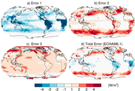
con-Figure 5. Maps of the impact of the three coding errors described in section 3.4 on the atmospheric energy budget, as well as the total error in the predecessor ECHAM6.1 model. The estimates shown here ignore the advection of cloud condensate.
densate, respectively. The total error in ECHAM6.1 of −0.03 W/m2is relatively small, which could explain why it remained undetected for many years. The problem, however, became apparent when the model was run into states far away from present-day conditions (Meraner et al., 2013; Popp et al., 2015, 2016; Voigt et al., 2011) resulted errors of several watts per square meter. Incidentally, the total error is almost identical to that of the revised model, ECHAM6.3, because errors of positive and negative signs almost cancel each other. Given the rather short integration time of only 1 year, the total error found in ECHAM6.3, with the advection of cloud condensate included, is due to incomplete cancellation on the regional scale, between the vertically integrated heating associated with phase changes of the water components on the one hand and the latent heat release by precipitation on the other hand (see equation (A10)). In the simulation with-out advection, the total error in ECHAM6.3 is virtually 0. The conservation properties were confirmed to hold also in warmer and colder states.
The regional error distributions, based on the simulations without advection of cloud condensate, are shown in Figure 5. The errors due to the inadequate discretization of the convective mass flux (Figure 5a) stand out particularly over the tropical continents. Smaller errors are found in the convective regimes over the low-latitude oceans and also in the midlatitude storm tracks. The negative sign in these regions implies that the vertically integrated heating due to phase changes of the water components (vapor, liquid, ice, rain, and snow) is smaller than the latent energy realized by rain and snow reaching the surface (see equation (A10)). On the other hand, the error caused by the inadequate treatment of the convective detrainment (Figure 5b) has a positive sign because the redefinition of the phase of the convective detrainment in the stratiform cloud condensation scheme ignores the energy required for the spurious melting of cloud ice generated in the convection scheme. This error is prominent particularly in the midlatitude storm tracks where it actually overcompensates the errors evident in Figure 5a. The positive sign of the error 3 implies that the surface heat flux is smaller than the diagnosed heating in the vertical column (Figure 5c). Due to error compensation (see the discussion of error 3 in Appendix A), the resulting error is small, except over snow-covered land where errors of up to 3 W/m2are found. The total error pattern in ECHAM6.1 (Figure 5d) is characterized by spurious atmospheric cooling at low latitudes, governed by error 1, and spurious atmospheric heating in the storm track regions governed by error 2. In ECHAM6.3 the individual errors as well as the total are either exactly 0 (error 3) or close to 0 (errors 1 and 2) at the grid point scale (not shown). Small residual errors can be explained by a nonzero storage of the cloud condensate, given the short integration time of 1 year in the here-presented experiments.
The fact that the atmosphere physics parameterizations now conserve energy does by no means guaran-tee conservation properties of the overall model system. Indeed, there are additional energy leakages in the atmosphere dynamical core, interpolation errors in the coupler near coastlines, neglect of the temperature of precipitation falling from the lowest model level into the ocean, and other minor errors. The overall leak-age of MPI-ESM1.2-LR is largely unchanged at around 0.45 W/m2as inferred from the top-of-atmosphere radiation balance in long control simulations. Some of these errors are reduced with higher resolution, but none of them vary appreciably with warming and so do not induce artificial feedbacks, which was a partic-ular concern in relation to past studies finding strongly increasing climate sensitivity in warmer climates (Heinemann et al., 2009; Meraner et al., 2013). Therefore, in section 8.3 we verify the nonlinearity properties of the model are retained after removing the coding errors.
3.5. Additional Modifications
In addition to the model revisions presented in sections 3.1 through 3.4, a few more features are changed: To achieve consistency with the rest of the model, a minor change was done in the convection scheme by replacing the specific heat of dry air by the specific heat of moist air.
The sea ice surface albedo and thermodynamics are calculated as part of the atmosphere whereas ice growth, melt, and advection is handled by the ocean in MPI-ESM1.2 (for details on this, see section 4). A bug in the sea ice melt pond scheme, relevant only in coupled model simulations, was identified and corrected (Roeckner et al., 2012): In the MPI-ESM (Giorgetta et al., 2013), melt ponds were accidentally ignored in the calculation of sea ice melt. Thus, the interaction between pond evolution, ice albedo, and ice melt was missing in the predecessor model. In MPI-ESM1.2 the melting of sea ice depends on the respective albedos of snow covered ice, bare ice, and melt ponds and on the respective fractional areas as well.
The subgrid scale mountain drag parameterization in ECHAM6.1 comprises the momentum transport from Earth's surface to the atmosphere accomplished by orographic gravity waves and, second, by the drag exerted by the subgrid scale mountains when the flow is blocked at low levels (Lott, 1999; Miller et al., 1989; Palmer et al., 1986). The strength of the gravity wave drag from unresolved orographic sources can be determined by parameters tuning the blocked flow drag amplitude (Cd) and the gravity wave stress amplitude (G), using the terminology of Lott (1999). In ECHAM6.1, the scheme was not activated at every grid point but only when two threshold values were exceeded characterizing rough terrain, that is, the standard deviation derived from the subgrid scale orography and the difference between the peak elevation and the mean elevation in the respective grid area. Thus, in addition to Cdand G, two more resolution-dependent tuning parameters were introduced in ECHAM6.1. This is avoided in ECHAM6.3 where the routine is activated at every grid point so that the results are now independent of the choice of the thresholds.
A related modification was made to the roughness length for momentum. In ECHAM6.1 this is a function of the subgrid scale orography and can be as large as 20 m. In ECHAM6.3 the roughness length for heat and momentum depends only on characteristics of the vegetation. Consequently, the momentum transport through vertical diffusion is systematically reduced over rough terrain, though compensated to some extent by an enhanced low-level flow blocking accomplished by a larger Cddiscussed above.
Furthermore, a bug in the definition of the land surface humidity was eliminated, the land surface albedo was slightly modified using MODIS data, and the land ice albedo (Greenland, Antarctica) has been decreased by about 5%, in better accordance with satellite data.
3.6. Atmospheric Model Tuning
A major retuning of the model was required because all modifications taken together caused a decrease of the global top-of-atmosphere radiation budget by about 10 W/m2due mainly to the corrected cloud fraction scheme (section 3.1) and also because the model climate sensitivity had roughly doubled to around 7 K, which would have prevented a reasonable match to the instrumental-record warming. If the latter had not been addressed, the model's historical warming would have roughly exceeded that observed by a factor of 2. When reducing the historical warming in a model there are essentially three options: reduce forcing, increase deep ocean heat uptake efficiency, or reduce the climate sensitivity. The forcing can be reduced by increasing aerosol cooling by enhancing the indirect effect, but at the time (2014–2015) we did not have such a parameterization in the model, which was developed after that (section 3.3). Further, ocean heat uptake already exceed that observed (Giorgetta et al., 2013), and so we were left with reducing the climate sensitivity. Since the predecessor MPI-ESM model warmed slightly more than observed, and it had a sensitivity of 3.5
K, we decided to aim at an equilibrium climate sensitivity of around 3 K. The reduction of the model's sensitivity was primarily achieved by increasing the entrainment rate for shallow convection by a factor of 10, from 3 × 10⁻⁴m−1in ECHAM6.1 to 3 × 10⁻³m−1in ECHAM6.3, with the purpose to reduce tropical low-level cloud feedback. But also other convective cloud parameters, mixed-phase cloud processes, and the representation of stratocumulus were found to be important.
After the corrections to the cloud fraction scheme (section 3.1), it turned out that the most efficient way to compensate for this radiation deficit is to reduce cloudiness by modifying the free parameters in the cloud fraction scheme. This was done by changing the profile parameters of the critical relative humidity (cf. equation (2)) from
{a1, a2, a3} = {0.7, 0.9, 4.0} to {0.75, 0.968, 1.0}, (6) so that cloud formation is systematically shifted to higher relative humidities. In addition, the optical thick-ness of low-level clouds is now parameterized as a function of cloud type. In the radiative transfer scheme, clouds are treated as plane parallel homogeneous layers defined by the cloud water path, CWP (liquid and/or ice). However, since real clouds are never homogeneous, it can be easily shown that the calculated reflectivity, for a given CWP, is always too high. This well-known bias can be attenuated to some extent by introducing a reduction factor (Cahalan et al., 1994), such that the CWP used in the radiation scheme is a fraction, fhom < 1, of that predicted by the cloud scheme, CWP = fhomCWPcld. In ECHAM6.1 fhomwas set to 0.77 for liquid water clouds and 0.8 for ice clouds. In ECHAM6.3 fhom = 0.8 for all cloud types, except for isolated shallow cumulus clouds, where fhom = 0.4 is applied as long as the CWP above cloud top is smaller than 20% of the total CWP. Such a distinction was suggested by Bäuml et al. (2004) who derived reduction factors for two cloud fields using data from cloud resolving simulations: a nocturnal marine stratocumulus case and a trade wind cumulus field.
A particular concern during the tuning of ECHAM6.3 was obtaining sufficient precipitation on tropical land, specifically in the Amazon and Sahel. This was long an issue in the model but with the increasing focus on the carbon cycle and the usage of dynamic vegetation the situation could no longer be ignored. The prob-lem applies foremost to the CR and LR configurations. Investigating the controls of precipitation on land in atmosphere-only simulations is complicated because a simple reduction in cloudiness will lead to warm-ing land surface temperatures, but the prescribed SSTs do not respond. Thus, in the tropics a direct thermal cell will drive more atmospheric moisture transport inland and thereby cause more precipitation on land, and therefore care must be taken to compensate the radiation balance. During our investigations, we found the problem to be robust to most changes, and the only parameter with a discernible effect is to increase critical relative humidity aloft (a1, equation (6)). This action, however, moves the parameter further from observational inference that favor even lower values (Quaas, 2012) and increases the equilibrium climate sensitivity away from the target. Thus, a fairly modest increase of a1was chosen. Additionally, the resis-tance to river-runoff in the hydrological discharge model was increased to further enhance the availability of groundwater to vegetation.
The tuning of the subgrid-scale orographic drag parameterization was further refined. For tuning, the strength of low-level blocking (Cd) and gravity wave stress (G) is used (section 3.5). In previous versions of the ECHAM model, these were set equal to simplify the tuning. However, we found that Cdis particularly important for controlling the flow over the Southern Ocean, whereas G was most effective in the Northern Hemisphere. A similar experience for another model is described in Pithan et al. (2016). By controlling the two parameters individually, it was possible to reduce sea level pressure and tropospheric zonal wind biases in the Southern Hemisphere substantially (see Appendix B).
4. Revisions of the Ocean Dynamics Model Component (MPIOM1.6)
Both the updated MPI-ESM1.1 and MPI-ESM1.2 model versions include the ocean component MPIOM1.6.3 and a sea ice model. These model components remained largely unchanged with respect to the MPI-ESM model version used during CMIP5 (for details, see Jungclaus et al., 2013; Notz et al., 2013). MPIOM is formulated on an Arakawa-C grid in the horizontal and on z levels in the vertical direction using the hydro-static and Boussinesq approximations. Subgrid-scale parameterizations include lateral mixing on isopycnals (Redi, 1982) and tracer transports by unresolved eddies (Gent et al., 1995). Vertical mixing is realized by a
combination of the Richardson number-dependent scheme of Pacanowski and Philander (1981) and directly wind-driven turbulent mixing in the mixed layer (for details see Jungclaus et al., 2013; Marsland et al., 2003). Variants of MPI-ESM1.2 differ in their ocean horizontal grids, where the MPI-ESM1.2-LR and the coarser MPI-ESM1.2-CR setups apply a bipolar grid, the HR, and higher-resolution configuration use a tripolar for-mulation, Table 1. The bipolar grids (GR1.5 in MPI-ESM1.2-LR and GR3.0 in MPI-ESM1.2-CR) feature one grid pole under Greenland and one under Antarctica. This choice causes regionally enhanced resolutions in the deepwater formation regions and the overflows across the Greenland-Scotland ridge. The tripolar grids allow for more uniform resolutions and are available in the TP04 version with eddy-permitting 0.4◦(as applied in MPI-ESM1.2-HR) and in the eddy-resolving TP6 m with a resolution of 6 min (MPI-ESM1.2-XR), as applied in the simulations of von Storch et al. (2012). In the vertical, 40 levels are unevenly placed in the water column, with the first 20 levels distributed over the top 700 m. The bottom topography is represented by a partial-step formulation (Wolff et al., 1997).
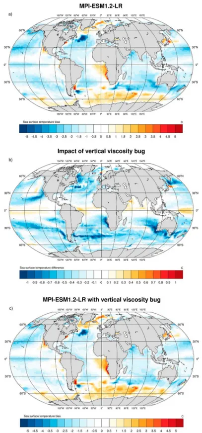
The MPIOM1.6.3 has been improved over earlier versions in terms of online diagnostics, meeting the requirements for OMIP (Griffies et al., 2016), and the flexibility of the model output. During the later stages of the preparation of MPI-ESM1.2, a coding error was discovered in the vertical viscosity scheme of MPIOM. Fixing this bug results in a considerable reduction of the SST biases in upwelling regions as well as in the Southern Ocean (Figures 6a and 6c) but also caused a slight surface cooling drift of about 0.2–0.3 K globally (Figure 6b). The latter required a small retuning of the model. Owing to various deadlines, MPI-ESM1.2-HR had already begun running its DECK runs and it was therefore deemed too late to implement the bug fix into MPI-ESM1.2-HR, but the LR version received this correction.
The sea ice model consists of code both in MPIOM and in ECHAM. In ECHAM, a simplified thermodynamic sea ice model is incorporated to provide at each atmospheric time step a physically consistent surface tem-perature in ice-covered regions. This part of the sea ice model contains a melt-pond scheme, which divides the surface of the sea ice into snow, bare ice, and melt pond, with each their individual albedo (Pedersen et al., 2009). In MPI-ESM1.2, these melt ponds are now fully activated, in contrast to an erroneous only par-tial activation in MPI-ESM (section 3.5, Roeckner et al., 2012). The atmospheric part of the sea ice model integrates all surface fluxes and provides at each coupling time step the gridded bulk surface flux into sea ice to the sea ice model in MPIOM. This surface flux is then used in MPIOM to calculate the sea ice sur-face energy balance and related changes in ice thickness. The thermodynamic description of sea ice is based on a simple zero-layer, mono-category formulation (Semtner, 1976). The differentiation of thermody-namic sea ice growth or melt between lateral processes that change ice concentration and vertical processes that change ice thickness is parameterised and can be adjusted by two tuning parameters (for details, see Mauritsen et al., 2012; Notz et al., 2013). These two parameters are used to tune the preindustrial Arctic sea ice volume of MPI-ESM1.2 to an annual average of roughly 20–25,000 km3. The values of the tuning param-eters are slightly adjusted in MPI-ESM1.2 relative to MPI-ESM to compensate for an otherwise too low sea ice volume.
For sea ice dynamics, MPI-ESM1.2 uses a viscoplastic rheology following Hibler (1979). This part of the sea ice model is also fully contained within MPIOM. At each coupling interval, MPIOM relates the updated sea ice thickness and sea ice concentration to ECHAM, which is then used there until the next coupling instance.
5. Revisions of the Ocean Carbon Cycle Model Component (HAMOCC6)
Processes represented in the Hamburg Ocean Carbon Cycle model are extended relative to that described in Ilyina et al. (2013) and parameters used in empirical relationships of existing processes are updated. As a new feature HAMOCC6 now resolves nitrogen-fixing cyanobacteria as an additional prognostic phytoplankton class (Paulsen et al., 2017). This replaces the diagnostic formulation of N2fixation applied in MPI-ESM-LR and allows the model to capture the response of N2fixation and ocean biogeochemistry to changing climate conditions. Updates of existing parameterized processes follow recommendations of the C4MIP and OMIP protocols (Jones et al., 2016; Orr et al., 2017).
5.1. Marine Nitrogen Fixation by Cyanobacteria
The parameterization of prognostic cyanobacteria as additional phytoplankton class is based on the phys-iological characteristics of the cyanobacterium Trichodesmium (Paulsen et al., 2017). Cyanobacteria in the model differ from bulk phytoplankton by their ability to grow on both nitrate (NO3) and dinitrogen (N2).
Fur-Figure 6. Sea surface temperature biases (50-year average) in preindustrial control simulations with respect to observed climatology (Steele et al., 2001): (a) MPI-ESM1.2-LR after applying the vertical viscosity bug fix and (c) the otherwise identical MPI-ESM1.2-LR but including the coding bug. (b) The difference between (a) and (c); (b) has a different color scale.
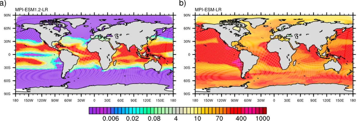
Figure 7. Dinitrogen (N2) fixation (𝜇mol N ·m−3·day−1) in preindustrial control simulations at the sea surface in (a)
the MPI-ESM1.2 version and (b) in the predecessor MPI-ESM model version used during CMIP5.
thermore, cyanobacteria have a slower maximum growth rate, are limited to a specific optimum temperature range, face a stronger iron limitation, and are positively buoyant. This way, modeled N2fixation is evolving in response to the combined effect of temperature, light, and nutrient distributions, that is, environmental conditions shaping cyanbacteria's ecological niche.
The implementation of prognostic cyanobacteria modifies the spatial distribution of N2fixation. In the diagnostic formulation, N2fixation was prescribed by a constant rate being active only in case of nitrate concentrations below the Redfield ratio (Ilyina et al., 2013). This resulted in unrealistically high N2fixation rates in high latitudes and a strong coupling of N2fixation to the nitrate-depleted regions overlying deni-trification sites, that is, in the eastern tropical Pacific, eastern tropical Atlantic, and in the northern Indian Ocean (Figure 7b). In MPI-ESM1.2 the abundance of cyanobacteria is the premise for N2fixation. Thus, fixation is restricted to the warm tropical and subtropical ocean, roughly between 40◦S and 40◦N, a result of temperature-limited cyanobacteria growth (Figure 7a). Furthermore, the availability of nutrients (iron and phosphate) and the competition with phytoplankton shape the areas of fixation. A detailed description of the parameterization and an evaluation of the representation of cyanobacteria and N2fixation against observations is given in Paulsen et al. (2017).
In MPI-ESM1.2, one modification was made to change the fate of dead cyanobacteria. The major fraction is considered as detritus and thus being affected by gravitational sinking. A small nonsinking fraction is con-sidered as dissolved organic matter (DOM), which in Paulsen et al. (2017) had a decay time of several years. In MPI-ESM1.2, this decay rate was reduced to several months, equivalent to that of the already existing DOM pool (being fed by phytoplankton). As sensitivity studies did not show considerable differences due to this rate parameter change, we combined both DOM pools to one at the benefit of lower computational cost. 5.2. Additional Changes and Bug Fixes
Previously, in HAMOCC, plankton dynamics were calculated only within the upper 100 m of the ocean, assuming low light availability would impede plankton growth below. This neglects grazing activity below 100 m and introduces temporally too high phytoplankton concentrations at depths after mixing below 100 m. Therefore, we now extend biological process calculations to the whole water column.
Detritus settling was modified by replacing the constant uniform settling rate of 5 m/day by a vertically varying settling rate based on observed particle fluxes (Martin et al., 1987). Martin and coauthors measured POC fluxes in the open ocean, found low spatial variability, and fitted the data to a normalized power law function. We implemented this fit by a depth-dependent settling velocity, which is 3.5 m/day within the upper 100 m and increases linearly below, up to 80 m/day at 6,000 m.
In HAMOCC6 we consider remineralization of organic material on dissolved oxygen, nitrate, nitrous oxide, and sulfate. Thereby, nutrients and dissolved inorganic carbon are released to the water column. Remineral-ization, as well, introduces changes to alkalinity, which depend on the composition of the organic material (i.e., the prescribed Redfield ratio in organic material) and the oxidation pathway. Previously, we assumed that alkalinity decreases during remineralization on sulfate. This would imply an instantaneous oxidation of hydrogen sulfide (H2S) being produced by sulfate reduction. However, as sulfate reduction occurs only under nearly anaerobic conditions H2S oxidation is unlikely to occur. Therefore, we introduced an
addi-Table 3
Parameter Setup for HAMOCC6 in Two Configurations of the MPI-ESM1.2 Model
Configuration HR LR
Parameter
Grazing rate (day−1) 0.7 1.0 Initial slope P-I curve (W−1·m2·day−1)
Bulk phytoplankton 0.04 0.025
Cyanobacteria 0.15 0.03
Cyanobacteria mortality rate (day−1) 0.04 0.10 Cyanobacteria half saturation constant for iron limitation (mmol∕m3) 0.6 0.8
Weathering rates
Organic material (kmol·P·s−1)a 5 4
DIC, alkalinity (kmol·C·s−1)b 537 428 Silicate (kmol·Si·s−1) 0 100
Note. Added as DOM, thus, all of N, P, Fe, O2, and C are added following the composition of organic material in HAMOCC6.
DIC and alkalinity are added in the ratio 1:2.
tional prognostic tracer (H2S), which is produced during remineralization on sulfate and decays only in oxygenated water. The purpose of H2S is to track alkalinity changes and to account for the local alkalin-ity increase due to sulfate reduction in oxygen minimum zones. However, this revision has only a minor impact (less than 1%0) on local alkalinity concentrations. This updated sulfate cycle is only implemented into MPI-ESM1.2-LR, while the MPI-ESM1.2-HR version did not receive this new feature (Table 3). With respect to remineralization we also reformulated the oxygen dependence for aerobic and anaerobic processes. In MPI-ESM there was a definite oxygen threshold value that limited aerobic remineralization (Ilyina et al., 2013). The corresponding turnover rate was independent of the ambient oxygen concentra-tion in the water. To allow for a gradual transiconcentra-tion between aerobic and anaerobic zones, we introduced a Monod kinetic type oxygen limitation𝛤oxywith a half saturation value of 10𝜇mol O2∕L. Thus, the aerobic remineralization rate decreases with decreasing dissolved oxygen concentration. As a complement, anaero-bic remineralization rates are modulated by (1 −𝛤oxy). All maximum remineralization rates and the critical oxygen concentration at which anaerobic processes start to occur are kept as in MPI-ESM.
Among other processes, primary production is a function of iron availability, which is mainly controlled by atmospheric dust deposition. In MPI-ESM1.2, the dust deposition climatology from Mahowald et al. (2006) is replaced with that of Mahowald et al. (2005). The latter has an overall lower input of dust and a slightly different spatial pattern, which we find preferable. Especially, the high dust deposition in the eastern Pacific of the Mahowald et al. (2006) climatology, which lead to excessive growth of cyanobacteria in the eastern equatorial Pacific, is alleviated in Mahowald et al. (2005), and hence, we reverted to the older climatology. In addition to scientifically motivated model refinement and bug fixes, we modified the parameter setup of several processes to comply to the agreements of protocols for model setup within CMIP6. In line with the OMIP protocol (Orr et al., 2017), we updated the formulation of the carbonate chemistry. In particular, we use the total pH scale and equilibrium constants recommended by (Dickson, 2010; Dickson et al., 2007). Fur-thermore, total alkalinity now additionally considers the alkalinity from phosphoric and silicic acid systems. Following the suggestions by the OMIP protocol (Orr et al., 2017), we updated the gas-exchange parame-terization. Now we use the gas transfer velocity formulation and parameter setup of Wanninkhof (2014). This includes updated Schmidt number parameterizations for CO2, O2, DMS, and N2O. To allow for sim-ulations with transient anthropogenic atmospheric nitrogen deposition within C4MIP (Jones et al., 2016), we implemented nitrogen deposition as an additional nitrate source. Wet and dry deposition of all nitrogen species (NOy+NHx) is directly used to update NO3, assuming instantaneous unlimited oxidation of NHxin
sea water. The corresponding H+ change is accounted for as an alkalinity decrease. Gridded coupled chem-istry model intercomparison N-deposition fields of version 1.0 are used as provided via the CMIP6 input database (https://esgf-node.llnl.gov/projects/input4mips/).