Parallel eigensolvers in plane-wave Density Functional Theory

HAL Id: hal-01323703

https://hal.archives-ouvertes.fr/hal-01323703

HAL is a multi-disciplinary open access

archive for the deposit and dissemination of sci-entific research documents, whether they are pub-lished or not. The documents may come from teaching and research institutions in France or abroad, or from public or private research centers.

L’archive ouverte pluridisciplinaire HAL, est destinée au dépôt et à la diffusion de documents scientifiques de niveau recherche, publiés ou non, émanant des établissements d’enseignement et de recherche français ou étrangers, des laboratoires publics ou privés.

Parallel eigensolvers in plane-wave Density Functional

Theory

Antoine Levitt, Marc Torrent

To cite this version:

Antoine Levitt, Marc Torrent. Parallel eigensolvers in plane-wave Density Functional Theory. Com-puter Physics Communications, Elsevier, 2015, 187, pp.98-105. �10.1016/j.cpc.2014.10.015�. �hal-01323703�

Parallel eigensolvers in plane-wave Density Functional Theory

Antoine Levitt∗, Marc Torrent

CEA, DAM, DIF, F-91297, Arpajon, France

Abstract

We consider the problem of parallelizing electronic structure computations in plane-wave Density Functional Theory. Because of the limited scalability of Fourier transforms, parallelism has to be found at the eigensolver level. We show how a recently proposed algorithm based on Chebyshev polynomials can scale into the tens of thousands of processors, outperforming block conjugate gradient algorithms for large computations.

Keywords: Density Functional Theory, ABINIT, Projector Augmented-Wave, Chebyshev filtering, LOBPCG, Woodbury formula

Contents

1 Introduction 2

2 The eigenvalue problem 3

2.1 The operators . . . 3

2.2 Solving the eigenvalue problem: conjugate gradient . . . 5

2.3 Block algorithms: LOBPCG . . . 5

3 Parallelism 6 3.1 Parallelism in the Hamiltonian application . . . 6

3.2 Eigenvector-level parallelism in block algorithms . . . 6

4 Chebyshev filtering 7 4.1 Filtering algorithms . . . 7

4.2 Chebyshev filtering . . . 9

5 Implementation 10 5.1 Inversion of the overlap matrix . . . 10

5.2 Parallelism . . . 11

5.3 Choice of the polynomial . . . 11

5.4 Locking . . . 12

∗

Corresponding author

Email addresses: antoine.levitt@gmail.com (Antoine Levitt), marc.torrent@cea.fr (Marc Torrent)

6 Results 13 6.1 Non-self-consistent convergence . . . 13 6.2 Self-consistent convergence . . . 14 6.3 Scalability . . . 17 7 Conclusion 17 1. Introduction

Kohn-Sham Density Functional Theory is an efficient way to solve the Schrödinger equation for quantum systems [13, 16]. By modelling the correlation between N electrons via exchange-correlation functionals, it leads to the Kohn-Sham system, mathematically formulated as a non-linear eigenvalue problem. This problem can be discretized and solved numerically, and the result of this computation allows the determination of physical properties of interest via higher-level processing such as geometry optimization, molecular dynamics or response-function computation. Density Functional Theory (DFT) codes can be classified according to the discretization scheme used to represent wavefunctions (plane waves, localized basis functions, finite differences ...) and the treatment of core electrons (all-electron computations, pseudopotentials ...). We focus on the ABINIT software [10], which uses a plane-wave basis and either norm-conserving pseudopotentials or the Projector Augmented-Wave (PAW) approach [5, 25].

The bottleneck of most simulations is the computation of the electronic ground state. This is done by a self-consistent cycle whose inner step is the solution of a linear eigenvalue problem. This step has to be implemented efficiently, taking into account the specificities of the problem at hand, which rules out the use of generic black-box solvers. Furthermore, the growing need for paralleliza-tion constrains the choice of the eigensolver. Indeed, one specificity of plane-wave DFT as opposed to real-space codes is that Fourier transforms do not scale beyond about 100 processors: effective parallelization requires eigensolvers that are able to compute several Hamiltonian applications in parallel.

The historic eigensolver used in plane-wave DFT, the conjugate gradient scheme of refs. [19, 17], is inherently sequential, although there are attempts at parallelization by omitting orthogonaliza-tions [14]. Several methods work on blocks of eigenvectors and are more suited for parallelization, such as the residual vector minimization – direct inversion in the iterative subspace (RMM-DIIS) scheme [17], and block Davidson algorithms [8], including the locally optimal block preconditioned conjugate gradient (LOBPCG) algorithm [15], implemented in ABINIT [6].

Parallel implementations of plane-wave DFT codes include Quantum Espresso [9], VASP [17], QBOX [11] or CASTEP [18]. The scalability of these codes is mainly limited by orthogonalizations and the Rayleigh-Ritz step, a dense matrix diagonalization, which is hard to parallelize efficiently, even using state-of-the-art libraries such as ELPA [1] or Elemental [21]. The Rayleigh-Ritz step usually becomes the bottleneck when using more than a thousand processors.

There are two main ways to decrease the cost of this step. One is to use it as rarely as possible. This usually means applying the Hamiltonian more than one time to each vector before applying the Rayleigh-Ritz procedure, in order to speed up convergence. The other is getting rid of it entirely. This requires the independent computation of parts of the spectrum, as in the methods of spectrum slicing [24] or of contour integrals [20, 23]. These approaches effectively solve an interior eigenvalue problem, which is considerably harder than the original exterior one. The result is that

a large number of Hamiltonian applications is needed, to obtain a high-degree polynomial or to solve linear systems.

While these spectrum decomposition techniques will surely become the dominant methods for exascale computing, we address the current generation of supercomputers, on which the decrease in the costs of the Rayleigh-Ritz step is not worth the great increase in the number of Hamiltonian applications. We therefore focus in this paper on the method of Chebyshev filtering, which aims to limit the number of Rayleigh-Ritz steps by applying polynomials of the Hamiltonian to each vector. It can be seen as an accelerated subspace iteration, and dates back to the RITZIT code in 1970 [22]. It has been proposed for use in DFT in refs. [28, 27], and has recently been adopted by several groups [4, 2].

The contribution of this paper is twofold. First, we show how to adapt the Chebyshev filtering algorithm of ref. [28] in the context of generalized eigenproblems, here due to the PAW formalism. By exploiting the particular nature of the PAW overlap matrix (a low-rank perturbation of the identity), we are able to invert it efficiently. Second, we compare the Chebyshev filtering algorithm with CG and LOBPCG, both in terms of convergence and scalability.

2. The eigenvalue problem

2.1. The operators

First, we define some relevant variables. For a system of Natoms atoms in a box, we solve the

Kohn-Sham equations in a plane-wave basis. This basis is defined by the set of all plane waves whose kinetic energy is less than a threshold Ecut. This yields a sphere of Npw plane waves, upon

which the wavefunctions are discretized.

We consider a system where N_bandsbands are sought. For a simple ground state computation,

Nbands represents the number of states occupied by valence electrons of the Natoms atoms. For

more sophisticated analysis such as Many-Body Perturbation Theory (MBPT), the computation of empty states is necessary, and N_bands can be significantly higher. It is also convenient to speed up convergence of ground state computations to use more bands than strictly necessary.

To account for the core electrons, we use pseudopotentials. ABINIT implements both norm-conserving pseudopotentials and the Projector Augmented-Wave (PAW) method. For the purposes of this paper, the main difference is the presence of an overlap matrix in the PAW case, leading to a generalized eigenvalue problem. We will assume in the rest of this paper that we use the PAW method: norm-conserving pseudopotentials follow as a special case.

For simplicity of notation, we consider in this paper the case where periodicity is not taken explicitely into account, and the wavefunctions will be assumed to be real. The following discussion extends to the periodic case by sampling of the Brillouin zone, provided that we consider complex eigenproblems, with the necessary adjustments.

The Kohn-Sham equations for the electronic wavefunctions ψnare

Hψn= λnSψn, (1)

where H is the Hamiltonian, and S the overlap matrix arising from the PAW method (S = I with norm-conserving pseudopotentials). H and S are N_pw × N_pw Hermitian matrices (although they are never formed explicitely), and Ψ is a Npw × Nbandsmatrix of wavefunctions. The Hamiltonian

operator depends self-consistently on the wavefunctions Ψ. It can be written in the form

The kinetic energy operator K is, in our plane wave basis, a simple diagonal matrix. The local operator V_loc = V_ext+ V_H+ V_XC is a multiplication in real space by a potential determined from atomic data and the wavefunctions Ψ. It can therefore be computed efficiently using a pair of inverse and direct FFTs. The nonlocal operator V_nonloc and the overlap matrix S depend on the atomic data used. For both PAW method and norm-conserving pseudopotentials, we introduce a set of

nlmn projectors per atom, where nlmn is the number of projectors used to model the core electrons

of each atom, and usually varies between 1 and 40 according to the atom and pseudopotential type. Therefore, for a homogeneous system of N_atoms atoms we use a total of N_projs= n_lmnNatoms

projectors. We have Nprojs Npw, but Nprojsis comparable to Nbands.

We gather formally these projectors in a N_pw× N_projsmatrix P . The non-local operator V_nonloc is computed as

Vnonloc = P DVPT. (3)

Similarly, the overlap matrix in the PAW formalism is

S = I + P DSPT. (4)

The matrices D_S and D_V do not couple the different atoms in the system: they are block-diagonal. They can be precomputed from atomic data. The matrix DV additionally depends

self-consistently on the wavefunctions Ψ.

Therefore, for a single band ψ, the process of computing Hψ and Sψ can be decomposed as follows

Input: a wavefunction ψ Output: Hψ, Sψ

◦ Compute Kψ by a simple scaling

◦ Apply an inverse FFT to ψ to compute its real-space representation, multiply by Vloc,

and apply a FFT to get V_locψ

◦ Compute the N_projsprojections p_ψ = PTψ

Apply the block-diagonal matrices DV and DS to pψ

Compute the contributions P D_Vpψ and P DSpψ to the nonlocal and overlap operator

◦ Assemble Hψ = Kψ + V_locψ + P DVpψ

◦ Assemble Sψ = ψ + P DSpψ

Algorithm 1: Computation of Hψ, Sψ

The total cost of this operation is O(N_pwlog N_pw+ N_pwNprojs). As Npw and Nprojs both scale

with the number of atoms Natoms, the cost of computing the non-local operator dominates for

large systems. However, N_pw is usually much greater than N_projs, and the prefactor involved in computing FFTs is much greater than the one involved in computing the simple matrix products

PTψ and P pψ (which can be efficiently implemented as a level-3 BLAS operation). The FFT and

non-local operator costs are usually of the same order of magnitude for systems up to about 50 atoms.

2.2. Solving the eigenvalue problem: conjugate gradient

The historical algorithm used to compute the N_bandsfirst eigenvectors of (1) in the framework of plane-wave DFT is the conjugate gradient algorithm, described in [19, 17]. It is mathematically based on the following variationnal characterization of the n-th eigenvector of the eigenproblem

Hψ = λSψ:

ψn= arg min

hψi,Sψi=δi,n, i=1,...,Npw

hψ, Hψi .

The conjugate gradient method of ref. [19, 17] consists of minimizing this functional by a projected conjugate gradient method. Note that, because of the constraints, this is a nonlinear conjugate gradient problem, to which classical (linear) results can not be applied. A number of desirable characteristics have made it the algorithm of reference.

First, this algorithm only needs the application of the operators H and S to wavefunctions, and can therefore be decoupled from their underlying structure. This is particularly suited to plane-wave Density Functional Theory, where the application of H can be efficiently computed with FFTs.

Second, the operator H = K + V_loc+ V_nonloc is closely approximated by K in the high-frequency regime. A good diagonal preconditionner can therefore be built by damping the high frequencies as

K−1above a certain threshold. The implementation in [19, 17], still used in most plane-wave codes, uses a smooth rational function with a variable threshold (typically taken to be the kinetic energy of the band under consideration). The use of a preconditionner greatly accelerates the convergence with only a negligible additional cost of O(Npw).

Third, the algorithm can naturally reuse approximate eigenvectors, in contrast to algorithms based on a growing basis such as the Lanczos iteration. This is extremely attractive in DFT computations, where very good approximations can be obtained from the previous self-consistent cycle.

Typically, this algorithm is implemented in the following way: for each band in ascending order, do a fixed number ninner of iterations of the conjugate gradient algorithm, orthogonalizing at each

step with respect to the other bands. Once every band is updated, use a Rayleigh-Ritz step (also called subspace rotation or subspace diagonalization), update the density (usually, Pulay mixing with preconditionning is used), and iterate until convergence. Therefore, one has a system of inner-outer iterations controlled by the variable n_inner. To our knowledge, little is known about the correct way to choose this parameter, especially if it is allowed to vary between bands.

2.3. Block algorithms: LOBPCG

A number of alternative approaches have been developed over the years. We focus in this section on the Locally-Optimal Block Preconditioned Conjugate Gradient (LOBPCG) algorithm [15], which was developed as a way to improve the convergence of the conjugate gradient method. In its single-block version, it consists of a Rayleigh-Ritz method in the 3N_bands-dimensional subspace spanned by the current trial wavefunctions, the wavefunctions computed at the previous iteration, and the (preconditionned) residuals. For a single band, this would be equivalent to the conjugate gradient algorithm. For multiple bands, by computing the eigenvectors as the solution to an eigenvalue problem in a well-chosen subspace, this method achieves higher convergence rates [15].

The price to pay for this faster convergence is the solution of a dense eigenvalue problem of size 3N_bands for the Rayleigh-Ritz method. While this cost is negligible for small systems, where

the cost of applying the Hamiltonian dominates the computation, its O(N_bands3 ) cost becomes problematic for larger systems, especially since it has poor parallel scaling. For this reason, a “multiblock” scheme has been implemented in ABINIT [6]. In this scheme, the Nbands bands are

split in N_blocks blocks. The LOBPCG algorithm is applied in each block, which is additionally kept orthogonal to the blocks of lower energy. In this way, the Rayleigh-Ritz cost is cut by a factor

N_blocks3 . The LOBPCG algorithm as described suffers from ill-conditioning of the matrices involved in the Rayleigh-Ritz step, and practical implementations have to be modified to use a more suitable basis (see [15, 12]), but the resulting method has proven robust and improves the convergence of the conjugate gradient algorithm.

The main advantage, and motivation of its adoption in ABINIT, is however not its improved convergence, but the ability to build the residuals for all the bands of a block in parallel, as will be discussed in the next section.

3. Parallelism

We consider the parallelization of ground state computations in plane-wave DFT, and its im-plementation in ABINIT.

3.1. Parallelism in the Hamiltonian application

The most straightforward way of parallelizing problem (1) is to use multiple processors to compute the Hamiltonian application Hψ needed in the conjugate gradient algorithm. In this approach, the vector ψ of size N_pw is distributed onto p_pw processors, and the Hamiltonian is computed in parallel. Although the non-local part can be computed very efficiently in this approach, the parallel computation of FFTs is a challenge. 3D FFT can be parallelized by computing multiple 2D FFTs in parallel, but this approach is intrinsically unable to exploit more than Npw1/3 processors.

Even for large systems, with Npw of about 1 million, this only amounts to using 100 processors,

which is clearly insufficient to use today’s supercomputers.

Therefore, in contrast with codes that work in a real-space localized basis, our delocalized basis is an obstacle to parallelism, limiting the scaling of the Hamiltonian application. To be used efficiently on supercomputers, parallelism must be found elsewhere.

3.2. Eigenvector-level parallelism in block algorithms

Another way of solving (1) in parallel is to use a block algorithm such as LOBPCG, in which the Hamiltonian application on the different vectors inside a block is done in parallel. This is the approach taken by ABINIT.

In this approach, the wavefunction matrix Ψ is distributed along a 2D grid of ppw × pbands

processors (see Figure 1). The Hamiltonian can be applied with only column-wise communica-tions between p_pw processors. The orthogonalization and Rayleigh-Ritz steps are done using a transposition to a (ppwpbands) × 1 processor grid. Implementation details can be found in [6].

Compared to using parallelism only in the Hamiltonian application, the scalability of the code is greatly extended, up to hundreds and even thousands of processors for large systems. The main obstacle to parallelism is the poor scalability of the Rayleigh-Ritz (subspace diagonalization) step. Even using parallel solvers such as ScaLAPACK [7] or ELPA [1], the diagonalization stops scaling at around 100 processors for large systems, and becomes the bottleneck when using many processors. Furthermore, as the blocksize has to be at least equal to pbands, as the number of processors increase,

Npw

Nbands

Figure 1: Distribution of the wavefunctions Ψ, with Nbands = 8, Npw = 10. The data is distributed on a 2D

processor grid of ppw = 2, pbands = 2. Each processor is in charge of Nblocks = 2 blocks of size Npw/ppw= 5 by

Nbands/pbands/Nblocks= 2.

To reduce these costs, we should ideally get rid of the global Rayleigh-Ritz step. This requires computing parts of the spectrum in parallel, which means solving an interior eigenvalue problem, requiring considerably more matrix-vector operations. An intermediate approach is to limit the number of global operations, i.e. to use several matrix-vector application for each Rayleigh-Ritz step.

4. Chebyshev filtering

4.1. Filtering algorithms

The filtering approach to eigenvalue problems emphasizes the invariant subspace spanned by the eigenvectors rather than the individual eigenvectors and eigenvalues. To obtain this invariant subspace, one uses a filter, an approximation of the spectral projector on the invariant subspace. Starting from an approximation to a basis of the invariant subspace, one applies the filter to each vector. Then, the basis is orthonormalized to prevent instability, and the process is iterated until convergence. Once a basis of the invariant subspace is obtained, a Rayleigh-Ritz procedure can be applied to recover the individual eigenvectors and eigenvalues.

This procedure can be seen as an accelerated version of the classical subspace iteration al-gorithm. This method is generally considered inferior to Krylov methods such as the Lanczos algorithm, but has a number of advantages that make it attractive in our context. First, it is able to use naturally the information of previous self-consistent iterations. Second, the filtering step can be done in parallel on each vector, with interaction between vectors only occuring in the Rayleigh-Ritz phase.

Another motivation for the use of filtering algorithms (see for instance [3]) is that, in many cases, one does not need the individual eigenvectors and eigenvalues, but aggregate quantities such as the density, that can be computed from any orthonormal basis. Therefore, one can avoid the Rayleigh-Ritz step altogether. We do not exploit this for two reasons. First, while this approach does avoid the dense diagonalization in the Rayleigh-Ritz step, it still requires an orthogonalization, which also scales poorly. Second, the algorithm becomes less stable, and provides less opportunities for error control (such as residuals) and locking. Third, it is not obvious how to accomodate occupation numbers, which, because of smearing schemes employed in computations of metals, depend self-consistently on the eigenvalues.

Several forms of filters have been proposed in the literature. [20] and [23] both use rational filters originating from discretizations of contour integrals to approximate the spectral projector. This is very efficient, provides numerous opportunities for parallelization and has the advantage of yielding “flat” filters, which have better stability properties. It is however inefficient in our case because it requires inversions of systems of the form (H − zS)x = b, where z is a complex shift. This becomes very poorly conditionned when the shift z becomes close to the real axis. Since our matrix is not sparse, one cannot rely on factorizations to solve these systems, and our tests have shown that solving these systems using iterative methods is too slow to be competitive.

Restricting ourselves to only Hamiltonian applications yields polynomial filters, that are less efficient but faster to compute than rational filters. Since we are looking for a filter that is minimal on the unwanted part of the spectrum, the natural idea is to use Chebyshev polynomials, as proposed in ref. [28]. This is the approach we take in this paper.

−2 −1.5 −1 −0.5 0 0.5 1 1.5 2 2.5 3 −0.2 0 0.2 0.4 0.6 0.8 1 1.2 Exact Chebyshev FEAST

Figure 2: Approximate filters to compute the [−1, 0] part of the full spectrum [−1, 2]. The Chebyshev polynomial is of degree 4, FEAST corresponds to the rational approximation of ref. [20] with 8 quadrature points (with symmetry, this amounts to 4 linear solves).

4.2. Chebyshev filtering

The Chebyshev polynomials have the property of being minimal in L∞ norm on an interval [a, b] among the polynomials of fixed degree and scaling. They are defined recursively by

T0(x) = 1, T1(x) = x − c r , Tn+1(x) = 2 x − c r Tn(x) − Tn−1(x),

where the filter center and radius are defined by

c = a + b

2 ,

r = b − a

2 .

This definition extends to any operator A and allows us to compute Tn(A)ψ using n applications

of A, and with only a modest additional memory cost.

If we denote by Λ and P the eigenvalues and eigenvectors of the eigenproblem Hψ = λSψ, then we have the decomposition HP = SP Λ, or S−1H = P ΛP−1. Therefore, Tn(S−1H)ψ =

P Tn(Λ)P−1ψ will have its eigencomponents filtered by the spectral filter Tn. We then use a

Rayleigh-Ritz procedure to separate the individual eigenvectors and eigenvalues, and iterate until convergence, as summarized in Algorithm 2.

Input: a set of Npw× N_bands wavefunctions Ψ

Output: the updated wavefunctions Ψ

◦ Compute Rayleigh quotients for every band, and set λ− equal to the largest one.

◦ Set λ+ to be an upper bound of the spectrum.

◦ Compute the filter center and radius c = λ++λ−

2 , r =

λ+−λ−

2 for each band ψ do

Set ψ0= ψ, and ψ1= 1_r(S−1Hψ0− cψ0₎ for i = 2, . . . , ninner do

ψi₌ 2

r(S

−1_Hψi−1_{− cψ}i−1_{) − ψ}i−2

end for end for

◦ Compute the subspace matrices H_ψ = ΨTHΨ, and SΨ= ΨTSΨ

◦ Solve the dense generalized eigenproblem HΨX = SΨXΛ, where Λ is a diagonal matrix

of eigenvalues, and X is the S_ψ-orthonormal set of eigenvectors ◦ Do the subspace rotation Ψ ← ΨX

Algorithm 2: Chebyshev filtering

This algorithm is identical to the one found in [28], except that, since we are dealing with a generalized eigenproblem, we need to apply a polynomial in S−1H instead of simply H. This

operator is not Hermitian, but has the same spectrum as the pencil (H, S), and the filtering algorithm finds the same eigenvectors and eigenvalues with the same convergence properties as in the Hermitian case. We will explain how to compute S−1 efficiently in Section 5.1.

5. Implementation

5.1. Inversion of the overlap matrix

We need to compute the operator S−1, where the overlap matrix S is given by

S = I + P DSPT.

This matrix is too large to invert directly, and is not even sparse. However, since N_projs N_pw, it is a low-rank perturbation of the identity. Therefore, we can apply the Woodbury formula [26] and write its inverse as

S−1= I − P (D−1_S + PTP )−1PT,

reducing the problem of computing the inverse of S to that of computing the inverse of the reduced

Nprojs× Nprojs matrix (D_S−1+ PTP ). This method for inverting S was also used in [? ] in the

context of preconditioning in ultrasoft computations.

In PAW, the projectors are compactly supported in spheres centered around the atoms. This leads us to expect that the matrix (D_S−1+ PTP ) is block-diagonal, and therefore easy to invert.

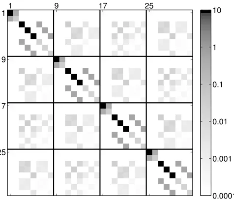
However, the projectors P are the discretization on the plane-wave basis of the true PAW projectors. Because a function cannot be compactly supported in both Fourier and real space, the plane-wave discretization of the projectors will spill over the neighbouring PAW spheres, and the Gram-matrix will have off-block diagonal entries (see Figure 3). This phenomenon is all the more pronounced when the projectors are not smooth (and therefore have slow Fourier-space decay), which is the case in many pseudopotentials commonly used (often constructed by imposing matching conditions).

The result of this is that the matrix (D_S−1+ PTP ) can not be considered block-diagonal, or

even sparse. While smaller than the full matrix S, it is still too large to invert directly in large systems. Therefore, we use an iterative solver, preconditionned by the block-diagonal component of (D−1_S + PTP ). Since the spillover phenomenon is relatively small, the preconditionner is a very

good approximation of the full matrix, and any iterative solver converges to machine precision in a relatively modest number of iterations. We used iterative refinement for its ease of implementation, although any symmetric indefinite solver such as MINRES could be used. In our tests, iterative refinement converged in about 10 to 20 iterations, depending on the energy cutoff of plane waves and the size of the PAW spheres. The cost of this inner iterative solver is O(N_projs2 ), and therefore small compared to the total cost O(NprojsNpw) of applying the overlap operator.

One inner iteration of CG or LOBPCG requires one multiplication by PT and two by P (one for H and one for S). Naively implemented, one inner iteration of the Chebyshev filter requires two multiplications by PT and two by P (one for H and one for S−1). However, we can avoid the multiplication by PT for H after the first iteration. Indeed, PTS−1ψ can be written as PTψ−PTP q,

where both PTψ and q have been computed before. By precomputing the Nprojs× Nprojs Gram

matrix PTP , this computation can be done in O(N_projs2 ) instead of the naive O(NprojsNpw).

Using this trick, the number of O(N_pw× N_projs) operations for the application of a Chebyshev filter of degree n is just one more as the number of such operations that would be necessary for n steps of a conjugate gradient algorithm. The iterative algorithm described has an additional cost of O(N_projs2 )  O(N_pw× N_projs). In our tests, we found that this additional cost per iteration compared to LOBPCG was largely compensated by the lack of orthogonalization: therefore, one step of Chebyshev filtering is a little faster than one step of LOBPCG.

1 9 17 25 1 9 17 25 0.0001 0.001 0.01 0.1 1 10

Figure 3: Projectors overlap matrix PTP (logarithmic color scale) for a system of 4 aluminium atoms in a periodic box,

with 8 projectors by atom. As an indication of the size of the overspill, denoting by M the preconditioner obtained by keeping only the 8 × 8 diagonal blocks, the condition number of M−1(PTP ) was 2.64, and the preconditionned

MINRES solver for the solution of PT_{P x = b with b a random vector converged to machine precision in 7 iterations.}

5.2. Parallelism

We have implemented this algorithm in the ABINIT software using MPI. The N_pw× N_bands eigenvector matrix is distributed on a 2D ppw× pbandsprocessors grid, in the same way as in [6]. We

apply the polynomial filter of degree n_inner, requiring communication inside the p_pwprocessor group for the FFT and the reductions needed for the nonlocal operator. Then, we transpose the data to a (ppwpbands) × 1 grid (using the MPI call MPI_ALLTOALL), build the submatrices, distribute them

between the processors and perform a Rayleigh-Ritz procedure. Note that, compared to LOBPCG, there is only one Rayleigh-Ritz per outer (self-consistent) iteration.

All our computations are done on the Curie supercomputer installed at the TGCC in France, a cluster of 16-core Intel processors with a total of about 80,000 processors. We used the Intel MKL library for BLAS and LAPACK dense linear algebra, and the ELPA library [1] for the dense eigenproblem in the Rayleigh-Ritz step (in our tests, we found it was about twice as fast as ScaLAPACK).

5.3. Choice of the polynomial

The choice of the polynomial degree ninner is a subtle matter, requiring a balance between

stability, speed and convergence.

First, a small degree results in many Rayleigh-Ritz steps, which is detrimental to performance, and especially to parallelism. On the other hand, if ninner is too large, we will solve very accurately

LOBPCG algorithms have showed that increasing n_inner above a moderate value (the default in ABINIT is 4) does not speed up the self-consistent cycle. The same goes for the Chebyshev filtering algorithm. More details are provided in Section 6.

Finally, if the degree is too large, the Gram matrix S_ψ will be ill-conditionned, even if the columns of Ψ are rescaled beforehand. This leads to loss of precision (and, crucially, of orthogo-nality). Therefore, we must have Tninner(

λ1−c

r )  1/ε, where Tn is the Chebyshev polynomial of

degree n, and ε ≈ 10−16 is the machine precision. In our tests, this was always the case except for large values of n_inner, of about 20, and therefore this instability is not an issue.

A key ingredient to the success of this algorithm is a good bracketing of the unwanted part of the spectrum. The authors in [28] propose a few steps of the Lanczos algorithms to compute an upper bound, but we simply use the upper bound E_cut on the kinetic energy of our system. It is not mathematically clear that this is an upper bound of the operator H = K + V , since V is not non-positive, but we have found this to be true in all our numerical tests.

To obtain an approximation of the smallest eigenvalue in the unwanted part of the spectrum, we use the maximum Rayleigh quotient (always an overestimation of the largest wanted eigenvalue

λNbands). We have found this to be more efficient than using the largest Ritz value of the previous

self-consistent iteration.

5.4. Locking

An important point for an effective implementation is the ability to lock converged eigenvectors, and not iterate on them. Although it is far from clear what the optimal policy is in terms of self-consistent convergence (how to optimize the number of iterations on each band to obtain the lowest total running time), it is desirable to stop the iterations prematurely in computations where a specified accuracy on the wavefunctions is desired.

In the Chebyshev algorithm, this means adaptatively choosing the degree of the polynomial, band per band. The problem is that there is no simple way to obtain a measure of the error while applying the polynomial: the vector being iterated on will become a combination of all the eigenvectors, and the size of its residual is meaningless before the Rayleigh-Ritz step. However, since an application of the Chebyshev polynomial of degree n enlarges the eigencomponent associated with eigenvalue λiby a factor Tn(λi_r−c), with the unwanted eigencomponents multiplied by a factor

of at most one, we can use the following approximation (which becomes exact at convergence) for the residual rn_i of band number i with Rayleigh quotient λ_i after one full Chebyshev iteration (application of a Chebyshev polynomial of degree n followed by a Rayleigh Ritz step)

krn_ik ≈ krik

Tn(λ1_r−c)

, (5)

where ri is the residual before the Chebyshev iteration (more details can be found in [? ] and in

references therein). Using this estimate, we can choose a priori the polynomial degree that will be needed to achieve a desired tolerance. This prediction can also be useful for other purposes, such as providing the user with an estimate of the progress of the computation.

Another issue is that using a polynomial of different degree for each band leads to systematic load imbalance between the processors: since the lower eigenvectors converge faster, the processors treating these will have less work than those treating the slow-converging higher eigenvectors. We avoid this by using a cyclic distribution of the bands between the processors, so that each processor treats a mix of low and high bands. This could be optimized further by redistributing dynamically

the bands so as to minimize the work imbalance, but we did not implement this as the simple cyclic distribution led to a load imbalance of less than 5% in our tests.

By contrast, the LOBPCG algorithm suffers from incomplete locking when a large number of processors is used, because the number of iteration has to be the same for each band in a block. Because of the dependence between the blocks, one cannot use a redistribution scheme such as in the Chebyshev algorithm. To keep the comparaison fair between Chebyshev and LOBPCG, we did not use any locking in the numerical results presented here.

6. Results

6.1. Non-self-consistent convergence

As a first test, we study the non-self-consistent convergence of our solver, meaning that we fix the Hamiltonian H and focus on the linear eigenvalue problem. Our test case is a system of 19 atoms of Barium titanate, with formula BaTiO₃, an insulator. We used an energy cutoff of 20 hartrees, representative of standard computations. With our PAW pseudopotential, there is a total of 77 totally filled bands. We run three algorithms: CG, the classical conjugate gradient of ref. [19, 17], the implementation of LOBPCG in ABINIT [6], and our Chebyshev algorithm. The full-block version of LOBPCG (Nblocks= 1) was used. In all cases, the parameter ninner, which controls

the number of inner iterations in all three algorithms, was set to 4. We monitor the convergence of all eigenpairs using their residual kHψ − λSψk.

−1.5 −1 −0.5 0 0.5 0 20 40 60 80 100 Eigenvalue λ Num b er of iterations Chebyshev CG LOBPCG

Figure 4: Number of iterations to obtain a precision of 10−10, BaTiO₃, 100 bands.

Figure 4 displays the number of iterations that was necessary for each eigenpair to attain an accuracy of 10−10, using a total of 100 bands. We see that the Chebyshev algorithm is very efficient

towards the bottom of the spectrum, outperforming the CG algorithm and even coming close to the full-block LOBPCG algorithm. However, the situation degrades for the upper eigenvalues, where the Chebyshev algorithm performs poorly, in part due to the intrinsically poorer performance of Chebyshev algorithms compared to Krylov methods, but in a large part due to the absence of pre-conditionner. In tests not shown here, Chebyshev consistently outperformed non-preconditionned CG and was competitive with non-preconditionned LOBPCG except for the last eigenpairs.

Figure 5 shows the exact same computation, but with 200 bands. First, note that increasing the number of bands yields improved convergence rates: the eigenpairs near 0.5 now converge in about 30 iterations for Chebyshev, whereas they did not converge in 100 iterations before. The inclusion of a large number of bands in the computation (200, compared with a total dimension of

Npw≈ 7000) also greatly enhances the effectiveness of the CG algorithm, although we do not fully

understand this effect. In this situation, the Chebyshev algorithm is not competitive.

−1.5 −1 −0.5 0 0.5 1 1.5 0 20 40 60 80 100 Eigenvalue λ Num b er of iterations Chebyshev CG LOBPCG

Figure 5: Number of iterations to get to obtain a precision of 10−10, BaTiO3, 200 bands.

We also note that the performance of the Chebyshev algorithm degrades like 1/√Ecut as the

energy cutoff is increased, whereas LOBPCG and CG, thanks to their preconditionning, only show a moderate increase in the number of iterations.

6.2. Self-consistent convergence

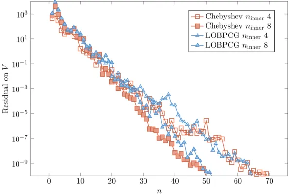
We now study the impact of the linear solver on the self-consistent cycle, and on the overall efficiency. Our tests are on a crystal of 256 atoms of Titanium. The partial occupation scheme used leads to about 1300 fully occupied bands and 500 partially occupied ones. We performed our tests with a total of 2048 bands.

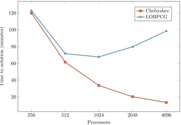
The computations were stopped when the residual on the potential went below 10−10. We report the convergence for n_inner equal to 4 and 8 in Figure 6. The results show that Chebyshev and LOBPCG are competitive on this system. The superior parallel performance of the Chebyshev algorithm yields large speedups when using more processors, as can be seen in Figure 7. In this case, taking the best time among all processor numbers yields a total time of about 15 minutes on 4096 processors for Chebyshev compared to more than an hour with 1024 processors for LOBPCG.

0 10 20 30 40 50 60 70 10−9 10−7 10−5 10−3 10−1 101 103 n Residual on V Chebyshev ninner 4 Chebyshev n_inner 8 LOBPCG n_inner 4 LOBPCG ninner 8

256 512 1024 2048 4096 20 40 60 80 100 120 Processors Time to solution (min utes) Chebyshev LOBPCG

Figure 7: Total time to solution. ninner was fixed to 4, and ppw to 32. The total number of iterations was 70 for

Chebyshev. It varied from 65 to 55 for LOBPCG, as the blocksize was increased from 32 on 256 processors to 512 on 4096.

6.3. Scalability

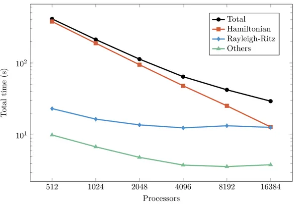
We now study more precisely the parallel scalability of our algorithms on a cristal of 512 atoms of Titanium, with a total of 4096 bands. We chose p_pw = 64. As before, we chose n_inner = 4. We measured the average running time of a single iteration. We began our measurements at 512 processors, and timed the individual routines. The speedups of Figure 8 are obtained with reference to a base case extrapolated by substracting the time spent in communications from the total time. The scalability for the Chebyshev algorithm is again much better, still scaling at 16384 proces-sors for the Ti₅₁₂ crystal when LOBPCG saturates at 2048. Figure 9 shows the breakdown of a step of the Chebyshev method. While the Hamiltonian application scales perfectly, as expected, the Rayleigh-Ritz step saturates very quickly and goes from negligible at 512 to being as costly as the Hamiltonian application at 16384 processors.

512 1024 2048 4096 8192 16384 512 1024 2048 4096 8192 16384 Processors Sp eedup Ideal Chebyshev LOBPCG

Figure 8: Speedups for the Chebyshev and LOBPCG method, Ti512.

7. Conclusion

Using a Woodbury decomposition of the PAW overlap matrix, we extended the Chebyshev filtering algorithm of [28, 27] to a generalized eigenproblem, and implemented it in the ABINIT software. Comparisons with the current implementation, based on the LOBPCG algorithm, show that its convergence properties are competitive for some systems, although it proves slower for

512 1024 2048 4096 8192 16384 101 102 Processors T otal time (s) Total Hamiltonian Rayleigh-Ritz Others

Figure 9: Breakdown of one step of the Chebyshev method, Ti₅₁₂.

others, due to its lack of preconditioning. Because it needs much less Rayleigh-Ritz steps, it is able to achieve much greater parallel speedups, and scale into the tens of thousands of processors.

This scaling behavior is acceptable for current generations of machines, where it is rare to be able to use more than 10,000 cores. However, exascale computations will only be possible with the help of algorithms that avoid global Rayleigh-Ritz steps. For plane-wave DFT, the only competitive algorithm seems to be the spectrum slicing algorithm of [24], but the high-degree polynomials it uses render it uncompetitive for all but extremely large systems. More research is needed to be able to develop alternatives.

Acknowledgements

We wish to thank Laurent Colombet for helpful discussions on HPC issues. Access to the Curie supercomputer was provided through the Centre de Calcul Recherche et Technologie (CCRT).

References

[1] T. Auckenthaler, V. Blum, H.-J. Bungartz, T. Huckle, R. Johanni, L. Krämer, B. Lang, H. Lederer, and P. R. Willems. Parallel solution of partial symmetric eigenvalue problems from electronic structure calculations. Parallel Computing, 37(12):783–794, 2011.

[2] A. S. Banerjee, R. S. Elliott, and R. D. James. A spectral scheme for kohn-sham density functional theory of clusters. arXiv preprint arXiv:1404.3773, 2014.

[3] C. Bekas, Y. Saad, M. L. Tiago, and J. R. Chelikowsky. Computing charge densities with partially reorthogonalized lanczos. Computer Physics Communications, 171(3):175–186, 2005. [4] M. Berljafa, D. Wortmann, and E. Di Napoli. An optimized and scalable eigensolver for

sequences of eigenvalue problems. arXiv preprint arXiv:1404.4161, 2014.

[5] P. E. Blöchl. Projector augmented-wave method. Physical Review B, 50(24):17953, 1994. [6] F. Bottin, S. Leroux, A. Knyazev, and G. Zérah. Large-scale ab initio calculations based on

three levels of parallelization. Computational Materials Science, 42(2):329–336, 2008.

[7] J. Choi, J. J. Dongarra, R. Pozo, and D. W. Walker. ScaLAPACK: A scalable linear alge-bra lialge-brary for distributed memory concurrent computers. In Frontiers of Massively Parallel

Computation, 1992., Fourth Symposium on the, pages 120–127. IEEE, 1992.

[8] E. R. Davidson. The iterative calculation of a few of the lowest eigenvalues and corresponding eigenvectors of large real-symmetric matrices. Journal of Computational Physics, 17(1):87–94, 1975.

[9] P. Giannozzi, S. Baroni, N. Bonini, M. Calandra, R. Car, C. Cavazzoni, D. Ceresoli, G. L. Chiarotti, M. Cococcioni, I. Dabo, et al. Quantum espresso: a modular and open-source software project for quantum simulations of materials. Journal of Physics: Condensed Matter, 21(39):395502, 2009.

[10] X. Gonze, B. Amadon, P.-M. Anglade, J.-M. Beuken, F. Bottin, P. Boulanger, F. Bruneval, D. Caliste, R. Caracas, M. Cote, et al. ABINIT: First-principles approach to material and nanosystem properties. Computer Physics Communications, 180(12):2582–2615, 2009.

[11] F. Gygi, E. W. Draeger, M. Schulz, B. R. De Supinski, J. A. Gunnels, V. Austel, J. C. Sexton, F. Franchetti, S. Kral, C. W. Ueberhuber, et al. Large-scale electronic structure calculations of high-z metals on the bluegene/l platform. In Proceedings of the 2006 ACM/IEEE conference

on Supercomputing, page 45. ACM, 2006.

[12] U. Hetmaniuk and R. Lehoucq. Basis selection in LOBPCG. Journal of Computational Physics, 218(1):324–332, 2006.

[13] P. Hohenberg and W. Kohn. Inhomogeneous electron gas. Physical review, 136(3B):B864, 1964.

[14] J.-I. Iwata, D. Takahashi, A. Oshiyama, T. Boku, K. Shiraishi, S. Okada, and K. Yabana. A massively-parallel electronic-structure calculations based on real-space density functional theory. Journal of Computational Physics, 229(6):2339–2363, 2010.

[15] A. V. Knyazev. Toward the optimal preconditioned eigensolver: Locally optimal block pre-conditioned conjugate gradient method. SIAM journal on scientific computing, 23(2):517–541, 2001.

[16] W. Kohn and L. J. Sham. Self-consistent equations including exchange and correlation effects.

[17] G. Kresse and J. Furthmüller. Efficient iterative schemes for ab initio total-energy calculations using a plane-wave basis set. Physical Review B, 54(16):11169, 1996.

[18] V. Milman, K. Refson, S. Clark, C. Pickard, J. Yates, S.-P. Gao, P. Hasnip, M. Probert, A. Perlov, and M. Segall. Electron and vibrational spectroscopies using dft, plane waves and pseudopotentials: Castep implementation. Journal of Molecular Structure: THEOCHEM, 954(1):22–35, 2010.

[19] M. C. Payne, M. P. Teter, D. C. Allan, T. Arias, and J. Joannopoulos. Iterative minimization techniques for ab initio total-energy calculations: molecular dynamics and conjugate gradients.

Reviews of Modern Physics, 64(4):1045–1097, 1992.

[20] E. Polizzi. Density-matrix-based algorithms for solving eigenvalue problems. Physical Review

B, 79(11):115112–115112, 2009.

[21] J. Poulson, B. Marker, R. A. van de Geijn, J. R. Hammond, and N. A. Romero. Elemental: A new framework for distributed memory dense matrix computations. ACM Transactions on

Mathematical Software (TOMS), 39(2):13, 2013.

[22] H. Rutishauser. Simultaneous iteration method for symmetric matrices. Numerische

Mathe-matik, 16(3):205–223, 1970.

[23] T. Sakurai and H. Sugiura. A projection method for generalized eigenvalue problems using numerical integration. Journal of computational and applied mathematics, 159(1):119–128, 2003.

[24] G. Schofield, J. R. Chelikowsky, and Y. Saad. A spectrum slicing method for the Kohn–Sham problem. Computer Physics Communications, 183(3):497–505, 2012.

[25] M. Torrent, F. Jollet, F. Bottin, G. Zérah, and X. Gonze. Implementation of the projector augmented-wave method in the ABINIT code: Application to the study of iron under pressure.

Computational Materials Science, 42(2):337–351, 2008.

[26] M. A. Woodbury. Inverting modified matrices. Memorandum report 42, Statistical Research

Group, Princeton, 1950.

[27] Y. Zhou, Y. Saad, M. L. Tiago, and J. R. Chelikowsky. Parallel self-consistent-field calculations via Chebyshev-filtered subspace acceleration. Phys. Rev. E, 74:066704, Dec 2006.

[28] Y. Zhou, Y. Saad, M. L. Tiago, and J. R. Chelikowsky. Self-consistent-field calculations using Chebyshev-filtered subspace iteration. Journal of Computational Physics, 219(1):172–184,