Characterization of the LIGO detectors
during their sixth science run
The MIT Faculty has made this article openly available.
Please share
how this access benefits you. Your story matters.
Citation
Aasi, J et al. “Characterization of the LIGO Detectors During Their
Sixth Science Run.” Classical and Quantum Gravity 32, 11 (May
2015): 115012 © IOP Publishing Ltd
As Published
http://dx.doi.org/10.1088/0264-9381/32/11/115012
Publisher
IOP Publishing
Version
Original manuscript
Citable link
https://hdl.handle.net/1721.1/121230
Terms of Use
Creative Commons Attribution-Noncommercial-Share Alike
sixth science run
J Aasi1, J Abadie1, B P Abbott1, R Abbott1, T Abbott2,
M R Abernathy1, T Accadia3, F Acernese4,5, C Adams6, T Adams7, R X Adhikari1, C Affeldt8, M Agathos9, N Aggarwal10, O D Aguiar11, P Ajith1, B Allen8,12,13, A Allocca14,15, E Amador Ceron12, D Amariutei16,
R A Anderson1, S B Anderson1, W G Anderson12, K Arai1, M C Araya1, C Arceneaux17, J Areeda18, S Ast13,
S M Aston6, P Astone19, P Aufmuth13, C Aulbert8,
L Austin1, B E Aylott20, S Babak21, P T Baker22,
G Ballardin23, S W Ballmer24, J C Barayoga1, D Barker25,
S H Barnum10, F Barone4,5, B Barr26, L Barsotti10,
M Barsuglia27, M A Barton25, I Bartos28, R Bassiri29,26,
A Basti14,30, J Batch25, J Bauchrowitz8, Th S Bauer9,
M Bebronne3, B Behnke21, M Bejger31, M.G Beker9,
A S Bell26, C Bell26, I Belopolski28, G Bergmann8,
J M Berliner25, A Bertolini9, D Bessis32, J Betzwieser6,
P T Beyersdorf33, T Bhadbhade29, I A Bilenko34, G Billingsley1, J Birch6, M Bitossi14, M A Bizouard35, E Black1, J K Blackburn1, L Blackburn36, D Blair37, M Blom9, O Bock8, T P Bodiya10, M Boer38, C Bogan8, C Bond20, F Bondu39, L Bonelli14,30, R Bonnand40, R Bork1, M Born8, S Bose41, L Bosi42, J Bowers2, C Bradaschia14,
P R Brady12, V B Braginsky34, M Branchesi43,44,
C A Brannen41, J E Brau45, J Breyer8, T Briant46,
D O Bridges6, A Brillet38, M Brinkmann8, V Brisson35,
M Britzger8, A F Brooks1, D A Brown24, D D Brown20,
F Br¨uckner20, T Bulik47, H J Bulten9,48, A Buonanno49,
D Buskulic3, C Buy27, R L Byer29, L Cadonati50,
G Cagnoli40, J Calder´on Bustillo51, E Calloni4,52,
J B Camp36, P Campsie26, K C Cannon53, B Canuel23,
J Cao54, C D Capano49, F Carbognani23, L Carbone20,
S Caride55, A Castiglia56, S Caudill12, M Cavagli`a17, F Cavalier35, R Cavalieri23, G Cella14, C Cepeda1, E Cesarini57, R Chakraborty1, T Chalermsongsak1,
S Chao58, P Charlton59, E Chassande-Mottin27, X Chen37, Y Chen60, A Chincarini61, A Chiummo23, H S Cho62, J Chow63, N Christensen64, Q Chu37, S S Y Chua63,
S Chung37, G Ciani16, F Clara25, D E Clark29, J A Clark50,
F Cleva38, E Coccia65,66, P.-F Cohadon46, A Colla19,67,
M Colombini42, M Constancio, Jr.11, A Conte19,67,
R Conte68, D Cook25, T R Corbitt2, M Cordier33,
N Cornish22, A Corsi69, C A Costa11, M W Coughlin70,
J.-P Coulon38, S Countryman28, P Couvares24,
D M Coward37, M Cowart6, D C Coyne1, K Craig26,
J D E Creighton12, T D Creighton32, S G Crowder71,
A Cumming26, L Cunningham26, E Cuoco23, K Dahl8,
T Dal Canton8, M Damjanic8, S L Danilishin37,
S D’Antonio57, K Danzmann8,13, V Dattilo23, B Daudert1,
H Daveloza32, M Davier35, G S Davies26, E J Daw72,
R Day23, T Dayanga41, G Debreczeni73, J Degallaix40,
E Deleeuw16, S Del´eglise46, W Del Pozzo9, T Denker8, T Dent8, H Dereli38, V Dergachev1, R De Rosa4,52, R T DeRosa2, R DeSalvo68, S Dhurandhar74, M D´ıaz32, A Dietz17, L Di Fiore4, A Di Lieto14,30, I Di Palma8, A Di Virgilio14, K Dmitry34, F Donovan10, K L Dooley8,
S Doravari6, M Drago75,76, R W P Drever77, J C Driggers1,
Z Du54, J -C Dumas37, S Dwyer25, T Eberle8, M Edwards7,
A Effler2, P Ehrens1, J Eichholz16, S S Eikenberry16,
G Endr˝oczi73, R Essick10, T Etzel1, K Evans26, M Evans10,
T Evans6, M Factourovich28, V Fafone57,66, S Fairhurst7,
Q Fang37, B Farr78, W Farr78, M Favata79, D Fazi78,
H Fehrmann8, D Feldbaum16,6, I Ferrante14,30, F Ferrini23,
F Fidecaro14,30, L S Finn80, I Fiori23, R Fisher24,
R Flaminio40, E Foley18, S Foley10, E Forsi6, L A Forte4,
N Fotopoulos1, J.-D Fournier38, S Franco35, S Frasca19,67,
F Frasconi14, M Frede8, M Frei56, Z Frei81, A Freise20, R Frey45, T T Fricke8, P Fritschel10, V V Frolov6, M.-K Fujimoto82, P Fulda16, M Fyffe6, J Gair70,
L Gammaitoni42,83, J Garcia25, F Garufi4,52, N Gehrels36, G Gemme61, E Genin23, A Gennai14, L Gergely81,
S Ghosh41, J A Giaime2,6, S Giampanis12, K D Giardina6,
A Giazotto14, S Gil-Casanova51, C Gill26, J Gleason16,
E Goetz8, R Goetz16, L Gondan81, G Gonz´alez2,
N Gordon26, M L Gorodetsky34, S Gossan60, S Goßler8,
R Gouaty3, C Graef8, P B Graff36, M Granata40, A Grant26,
S Gras10, C Gray25, R J S Greenhalgh84, A M Gretarsson85,
C Griffo18, H Grote8, K Grover20, S Grunewald21,
G M Guidi43,44, C Guido6, K E Gushwa1, E K Gustafson1,
R Gustafson55, B Hall41, E Hall1, D Hammer12,
G Hammond26, M Hanke8, J Hanks25, C Hanna86,
J Hanson6, J Harms1, G M Harry87, I W Harry24, E D Harstad45, M T Hartman16, K Haughian26,
K Hayama82, J Heefner†,1, A Heidmann46, M Heintze16,6, H Heitmann38, P Hello35, G Hemming23, M Hendry26, I S Heng26, A W Heptonstall1, M Heurs8, S Hild26,
D Hoak50, K A Hodge1, K Holt6, T Hong60, S Hooper37,
T Horrom88, D J Hosken89, J Hough26, E J Howell37,
Y Hu26, Z Hua54, V Huang58, E A Huerta24, B Hughey85,
J Iafrate2, D R Ingram25, R Inta63, T Isogai10, A Ivanov1,
B R Iyer90, K Izumi25, M Jacobson1, E James1, H Jang91,
Y J Jang78, P Jaranowski92, F Jim´enez-Forteza51,
W W Johnson2, D Jones25, D I Jones93, R Jones26,
R.J.G Jonker9, L Ju37, Haris K94, P Kalmus1,
V Kalogera78, S Kandhasamy71, G Kang91, J B Kanner36,
M Kasprzack23,35, R Kasturi95, E Katsavounidis10,
W Katzman6, H Kaufer13, K Kaufman60, K Kawabe25,
S Kawamura82, F Kawazoe8, F K´ef´elian38, D Keitel8,
D B Kelley24, W Kells1, D G Keppel8, A Khalaidovski8,
F Y Khalili34, E A Khazanov96, B K Kim91, C Kim97,91, K Kim98, N Kim29, W Kim89, Y.-M Kim62, E J King89, P J King1, D L Kinzel6, J S Kissel10, S Klimenko16,
J Kline12, S Koehlenbeck8, K Kokeyama2, V Kondrashov1, S Koranda12, W Z Korth1, I Kowalska47, D Kozak1,
A Kremin71, V Kringel8, B Krishnan8, A Kr´olak99,100,
C Kucharczyk29, S Kudla2, G Kuehn8, A Kumar101,
D Nanda Kumar16, P Kumar24, R Kumar26,
R Kurdyumov29, P Kwee10, M Landry25, B Lantz29,
S Larson102, P D Lasky103, C Lawrie26, A Lazzarini1,
P Leaci21, E O Lebigot54, C.-H Lee62, H K Lee98,
H M Lee97, J Lee10, J Lee18, M Leonardi75,76, J R Leong8,
A Le Roux6, N Leroy35, N Letendre3, B Levine25,
J B Lewis1, V Lhuillier25, T G F Li9, A C Lin29,
T B Littenberg78, V Litvine1, F Liu104, H Liu7, Y Liu54,
Z Liu16, D Lloyd1, N A Lockerbie105, V Lockett18, D Lodhia20, K Loew85, J Logue26, A L Lombardi50, M Lorenzini65, V Loriette106, M Lormand6, G Losurdo43, J Lough24, J Luan60, M J Lubinski25, H L¨uck8,13,
A P Lundgren8, J Macarthur26, E Macdonald7,
B Machenschalk8, M MacInnis10, D M Macleod7,
F Magana-Sandoval18, M Mageswaran1, K Mailand1,
E Majorana19, I Maksimovic106, V Malvezzi57, N Man38,
G M Manca8, I Mandel20, V Mandic71, V Mangano19,67,
M Mantovani14, F Marchesoni42,107, F Marion3, S M´arka28,
Z M´arka28, A Markosyan29, E Maros1, J Marque23,
F Martelli43,44, L Martellini38, I W Martin26,
R M Martin16, D Martynov1, J N Marx1, K Mason10,
A Masserot3, T J Massinger24, F Matichard10, L Matone28,
R A Matzner108, N Mavalvala10, G May2, N Mazumder94,
G Mazzolo8, R McCarthy25, D E McClelland63,
S C McGuire109, G McIntyre1, J McIver50, D Meacher38, G D Meadors55, M Mehmet8, J Meidam9, T Meier13, A Melatos103, G Mendell25, R A Mercer12, S Meshkov1, C Messenger26, M S Meyer6, H Miao60, C Michel40,
E E Mikhailov88, L Milano4,52, J Miller63, Y Minenkov57,
C M F Mingarelli20, S Mitra74, V P Mitrofanov34,
G Mitselmakher16, R Mittleman10, B Moe12, M Mohan23,
G Moreno25, N Morgado40, T Mori82, S R Morriss32,
K Mossavi8, B Mours3, C M Mow-Lowry8, C L Mueller16,
G Mueller16, S Mukherjee32, A Mullavey2, J Munch89,
D Murphy28, P G Murray26, A Mytidis16, M F Nagy73,
I Nardecchia19,67, T Nash1, L Naticchioni19,67, R Nayak110,
V Necula16, I Neri42,83, G Newton26, T Nguyen63,
E Nishida82, A Nishizawa82, A Nitz24, F Nocera23,
D Nolting6, M E Normandin32, L K Nuttall7, E Ochsner12,
J O’Dell84, E Oelker10, G H Ogin1, J J Oh111, S H Oh111,
F Ohme7, P Oppermann8, B O’Reilly6,
W Ortega Larcher32, R O’Shaughnessy12, C Osthelder1, C D Ott60, D J Ottaway89, R S Ottens16, J Ou58, H Overmier6, B J Owen80, C Padilla18, A Pai94, C Palomba19, Y Pan49, C Pankow12, F Paoletti14,23, R Paoletti14,15, M A Papa21,12, H Paris25, A Pasqualetti23,
R Passaquieti14,30, D Passuello14, M Pedraza1, P Peiris56,
S Penn95, A Perreca24, M Phelps1, M Pichot38,
M Pickenpack8, F Piergiovanni43,44, V Pierro68, L Pinard40,
B Pindor103, I M Pinto68, M Pitkin26, J Poeld8,
R Poggiani14,30, V Poole41, C Poux1, V Predoi7,
T Prestegard71, L R Price1, M Prijatelj8, M Principe68,
S Privitera1, G A Prodi75,76, L Prokhorov34, O Puncken32,
M Punturo42, P Puppo19, V Quetschke32, E Quintero1,
R Quitzow-James45, F J Raab25, D S Rabeling9,48, I R´acz73,
H Radkins25, P Raffai28,81, S Raja112, G Rajalakshmi113,
M Rakhmanov32, C Ramet6, P Rapagnani19,67, V Raymond1, V Re57,66, C M Reed25, T Reed114, T Regimbau38, S Reid115, D H Reitze1,16, F Ricci19,67, R Riesen6, K Riles55, N A Robertson1,26, F Robinet35, A Rocchi57, S Roddy6, C Rodriguez78, M Rodruck25,
C Roever8, L Rolland3, J G Rollins1, R Romano4,5,
G Romanov88, J H Romie6, D Rosi´nska31,116, S Rowan26,
A R¨udiger8, P Ruggi23, K Ryan25, F Salemi8, L Sammut103,
V Sandberg25, J Sanders55, V Sannibale1,
I Santiago-Prieto26, E Saracco40, B Sassolas40,
B S Sathyaprakash7, P R Saulson24, R Savage25,
R Schilling8, R Schnabel8,13, R M S Schofield45,
E Schreiber8, D Schuette8, B Schulz8, B F Schutz21,7,
P Schwinberg25, J Scott26, S M Scott63, F Seifert1,
D Sellers6, A S Sengupta117, D Sentenac23, A Sergeev96,
D Shaddock63, S Shah118,9, M S Shahriar78, M Shaltev8, B Shapiro29, P Shawhan49, D H Shoemaker10, T L Sidery20, K Siellez38, X Siemens12, D Sigg25, D Simakov8, A Singer1, L Singer1, A M Sintes51, G R Skelton12, B J J Slagmolen63, J Slutsky8, J R Smith18, M R Smith1, R J E Smith20,
N D Smith-Lefebvre1, K Soden12, E J Son111, B Sorazu26,
T Souradeep74, L Sperandio57,66, A Staley28, E Steinert25,
J Steinlechner8, S Steinlechner8, S Steplewski41,
S Strigin34, A S Stroeer32, R Sturani43,44, A L Stuver6,
T Z Summerscales119, S Susmithan37, P J Sutton7,
B Swinkels23, G Szeifert81, M Tacca27, D Talukder45,
L Tang32, D B Tanner16, S P Tarabrin8, R Taylor1,
A P M ter Braack9, M P Thirugnanasambandam1,
M Thomas6, P Thomas25, K A Thorne6, K S Thorne60,
E Thrane1, V Tiwari16, K V Tokmakov105, C Tomlinson72,
A Toncelli14,30, M Tonelli14,30, O Torre14,15, C V Torres32,
C I Torrie1,26, F Travasso42,83, G Traylor6, M Tse28,
D Ugolini120, C S Unnikrishnan113, H Vahlbruch13,
G Vajente14,30, M Vallisneri60, J F J van den Brand9,48, C Van Den Broeck9, S van der Putten9,
M V van der Sluys78, J van Heijningen9, A A van Veggel26, S Vass1, M Vas´uth73, R Vaulin10, A Vecchio20,
G Vedovato121, J Veitch9, P J Veitch89, K Venkateswara122,
D Verkindt3, S Verma37, F Vetrano43,44, A Vicer´e43,44,
R Vincent-Finley109, J.-Y Vinet38, S Vitale10,9, B Vlcek12,
T Vo25, H Vocca42,83, C Vorvick25, W D Vousden20,
D Vrinceanu32, S P Vyachanin34, A Wade63, L Wade12,
M Wade12, S J Waldman10, M Walker2, L Wallace1,
Y Wan54, J Wang58, M Wang20, X Wang54, A Wanner8,
R L Ward63, M Was8, B Weaver25, L.-W Wei38,
M Weinert8, A J Weinstein1, R Weiss10, T Welborn6,
L Wen37, P Wessels8, M West24, T Westphal8, K Wette8,
J T Whelan56, S E Whitcomb1,37, D J White72,
B F Whiting16, S Wibowo12, K Wiesner8, C Wilkinson25, L Williams16, R Williams1, T Williams123, J L Willis124, B Willke8,13, M Wimmer8, L Winkelmann8, W Winkler8, C C Wipf10, H Wittel8, G Woan26, J Worden25, J Yablon78, I Yakushin6, H Yamamoto1, C C Yancey49, H Yang60,
D Yeaton-Massey1, S Yoshida123, H Yum78, M Yvert3,
A Zadro ˙zny100, M Zanolin85, J.-P Zendri121, F Zhang10,
L Zhang1, C Zhao37, H Zhu80, X J Zhu37, N Zotov‡,114,
M E Zucker10, and J. Zweizig1
1LIGO - California Institute of Technology, Pasadena, CA 91125, USA
2Louisiana State University, Baton Rouge, LA 70803, USA
3Laboratoire d’Annecy-le-Vieux de Physique des Particules (LAPP), Universit´e
de Savoie, CNRS/IN2P3, F-74941 Annecy-le-Vieux, France
4INFN, Sezione di Napoli, Complesso Universitario di Monte S.Angelo, I-80126
Napoli, Italy
5Universit`a di Salerno, Fisciano, I-84084 Salerno, Italy
6LIGO - Livingston Observatory, Livingston, LA 70754, USA
7Cardiff University, Cardiff, CF24 3AA, United Kingdom
8Albert-Einstein-Institut, Max-Planck-Institut f¨ur Gravitationsphysik, D-30167
Hannover, Germany
9Nikhef, Science Park, 1098 XG Amsterdam, The Netherlands
10LIGO - Massachusetts Institute of Technology, Cambridge, MA 02139, USA
11Instituto Nacional de Pesquisas Espaciais, 12227-010 - S˜ao Jos´e dos Campos,
SP, Brazil
12University of Wisconsin–Milwaukee, Milwaukee, WI 53201, USA
13Leibniz Universit¨at Hannover, D-30167 Hannover, Germany
15Universit`a di Siena, I-53100 Siena, Italy
16University of Florida, Gainesville, FL 32611, USA
17The University of Mississippi, University, MS 38677, USA
18California State University Fullerton, Fullerton, CA 92831, USA
19INFN, Sezione di Roma, I-00185 Roma, Italy
20University of Birmingham, Birmingham, B15 2TT, United Kingdom
21Albert-Einstein-Institut, Max-Planck-Institut f¨ur Gravitationsphysik, D-14476
Golm, Germany
22Montana State University, Bozeman, MT 59717, USA
23European Gravitational Observatory (EGO), I-56021 Cascina, Pisa, Italy
24Syracuse University, Syracuse, NY 13244, USA
25LIGO - Hanford Observatory, Richland, WA 99352, USA
26SUPA, University of Glasgow, Glasgow, G12 8QQ, United Kingdom
27APC, AstroParticule et Cosmologie, Universit´e Paris Diderot, CNRS/IN2P3,
CEA/Irfu, Observatoire de Paris, Sorbonne Paris Cit´e, 10, rue Alice Domon et
L´eonie Duquet, F-75205 Paris Cedex 13, France
28Columbia University, New York, NY 10027, USA
29Stanford University, Stanford, CA 94305, USA
30Universit`a di Pisa, I-56127 Pisa, Italy
31CAMK-PAN, 00-716 Warsaw, Poland
32The University of Texas at Brownsville, Brownsville, TX 78520, USA
33San Jose State University, San Jose, CA 95192, USA
34Moscow State University, Moscow, 119992, Russia
35LAL, Universit´e Paris-Sud, IN2P3/CNRS, F-91898 Orsay, France
36NASA/Goddard Space Flight Center, Greenbelt, MD 20771, USA
37University of Western Australia, Crawley, WA 6009, Australia
38ARTEMIS, Universit´e Nice-Sophia-Antipolis, CNRS and Observatoire de la
Cˆote d’Azur, F-06304 Nice, France
39Institut de Physique de Rennes, CNRS, Universit´e de Rennes 1, F-35042
Rennes, France
40Laboratoire des Mat´eriaux Avanc´es (LMA), IN2P3/CNRS, Universit´e de
Lyon, F-69622 Villeurbanne, Lyon, France
41Washington State University, Pullman, WA 99164, USA
42INFN, Sezione di Perugia, I-06123 Perugia, Italy
43INFN, Sezione di Firenze, I-50019 Sesto Fiorentino, Firenze, Italy
44Universit`a degli Studi di Urbino ’Carlo Bo’, I-61029 Urbino, Italy
45University of Oregon, Eugene, OR 97403, USA
46Laboratoire Kastler Brossel, ENS, CNRS, UPMC, Universit´e Pierre et Marie
Curie, F-75005 Paris, France
47Astronomical Observatory Warsaw University, 00-478 Warsaw, Poland
48VU University Amsterdam, 1081 HV Amsterdam, The Netherlands
49University of Maryland, College Park, MD 20742, USA
50University of Massachusetts - Amherst, Amherst, MA 01003, USA
51Universitat de les Illes Balears, E-07122 Palma de Mallorca, Spain
52Universit`a di Napoli ’Federico II’, Complesso Universitario di Monte S.Angelo,
I-80126 Napoli, Italy
53Canadian Institute for Theoretical Astrophysics, University of Toronto,
Toronto, Ontario, M5S 3H8, Canada
54Tsinghua University, Beijing 100084, China
55University of Michigan, Ann Arbor, MI 48109, USA
56Rochester Institute of Technology, Rochester, NY 14623, USA
57INFN, Sezione di Roma Tor Vergata, I-00133 Roma, Italy
58National Tsing Hua University, Hsinchu Taiwan 300
59Charles Sturt University, Wagga Wagga, NSW 2678, Australia
60Caltech-CaRT, Pasadena, CA 91125, USA
61INFN, Sezione di Genova, I-16146 Genova, Italy
62Pusan National University, Busan 609-735, Korea
63Australian National University, Canberra, ACT 0200, Australia
64Carleton College, Northfield, MN 55057, USA
65INFN, Gran Sasso Science Institute, I-67100 L’Aquila, Italy
67Universit`a di Roma ’La Sapienza’, I-00185 Roma, Italy
68University of Sannio at Benevento, I-82100 Benevento, Italy and INFN
(Sezione di Napoli), Italy
69The George Washington University, Washington, DC 20052, USA
70University of Cambridge, Cambridge, CB2 1TN, United Kingdom
71University of Minnesota, Minneapolis, MN 55455, USA
72The University of Sheffield, Sheffield S10 2TN, United Kingdom
73Wigner RCP, RMKI, H-1121 Budapest, Konkoly Thege Mikl´os ´ut 29-33,
Hungary
74Inter-University Centre for Astronomy and Astrophysics, Pune - 411007, India
75INFN, Gruppo Collegato di Trento, I-38050 Povo, Trento, Italy
76Universit`a di Trento, I-38050 Povo, Trento, Italy
77California Institute of Technology, Pasadena, CA 91125, USA
78Northwestern University, Evanston, IL 60208, USA
79Montclair State University, Montclair, NJ 07043, USA
80The Pennsylvania State University, University Park, PA 16802, USA
81MTA-Eotvos University, ‘Lendulet’A. R. G., Budapest 1117, Hungary
82National Astronomical Observatory of Japan, Tokyo 181-8588, Japan
83Universit`a di Perugia, I-06123 Perugia, Italy
84Rutherford Appleton Laboratory, HSIC, Chilton, Didcot, Oxon, OX11 0QX,
United Kingdom
85Embry-Riddle Aeronautical University, Prescott, AZ 86301, USA
86Perimeter Institute for Theoretical Physics, Ontario, N2L 2Y5, Canada
87American University, Washington, DC 20016, USA
88College of William and Mary, Williamsburg, VA 23187, USA
89University of Adelaide, Adelaide, SA 5005, Australia
90Raman Research Institute, Bangalore, Karnataka 560080, India
91Korea Institute of Science and Technology Information, Daejeon 305-806,
Korea
92Bia lystok University, 15-424 Bia lystok, Poland
93University of Southampton, Southampton, SO17 1BJ, United Kingdom
94IISER-TVM, CET Campus, Trivandrum Kerala 695016, India
95Hobart and William Smith Colleges, Geneva, NY 14456, USA
96Institute of Applied Physics, Nizhny Novgorod, 603950, Russia
97Seoul National University, Seoul 151-742, Korea
98Hanyang University, Seoul 133-791, Korea
99IM-PAN, 00-956 Warsaw, Poland
100NCBJ, 05-400 ´Swierk-Otwock, Poland
101Institute for Plasma Research, Bhat, Gandhinagar 382428, India
102Utah State University, Logan, UT 84322, USA
103The University of Melbourne, Parkville, VIC 3010, Australia
104University of Brussels, Brussels 1050 Belgium
105SUPA, University of Strathclyde, Glasgow, G1 1XQ, United Kingdom
106ESPCI, CNRS, F-75005 Paris, France
107Universit`a di Camerino, Dipartimento di Fisica, I-62032 Camerino, Italy
108The University of Texas at Austin, Austin, TX 78712, USA
109Southern University and A&M College, Baton Rouge, LA 70813, USA
110IISER-Kolkata, Mohanpur, West Bengal 741252, India
111National Institute for Mathematical Sciences, Daejeon 305-390, Korea
112RRCAT, Indore MP 452013, India
113Tata Institute for Fundamental Research, Mumbai 400005, India
114Louisiana Tech University, Ruston, LA 71272, USA
115SUPA, University of the West of Scotland, Paisley, PA1 2BE, United
Kingdom
116Institute of Astronomy, 65-265 Zielona G´ora, Poland
117Indian Institute of Technology, Gandhinagar Ahmedabad Gujarat 382424,
India
118Department of Astrophysics/IMAPP, Radboud University Nijmegen, P.O.
Box 9010, 6500 GL Nijmegen, The Netherlands
119Andrews University, Berrien Springs, MI 49104, USA
121INFN, Sezione di Padova, I-35131 Padova, Italy
122University of Washington, Seattle, WA 98195, USA
123Southeastern Louisiana University, Hammond, LA 70402, USA
124Abilene Christian University, Abilene, TX 79699, USA
†Deceased, April 2012.
‡Deceased, May 2012.
Abstract. In 2009-2010, the Laser Interferometer Gravitational-wave
Observa-tory (LIGO) operated together with international partners Virgo and GEO600 as a network to search for gravitational waves of astrophysical origin. The sensitiv-ity of these detectors was limited by a combination of noise sources inherent to the instrumental design and its environment, often localized in time or frequency, that couple into the gravitational-wave readout. Here we review the performance of the LIGO instruments during this epoch, the work done to characterize the de-tectors and their data, and the effect that transient and continuous noise artefacts have on the sensitivity of LIGO to a variety of astrophysical sources.
PACS numbers: 04.80.Nn.
1. Introduction
Between July 2009 and October 2010, the Laser Interferometer Gravitational-wave Observatory (LIGO) [1] operated two 4-kilometre laser interferometers as part of a global network aiming to detect and study gravitational waves (GWs) of astrophysical origin. These detectors, at LIGO Hanford Observatory, WA (LHO), and LIGO Livingston Observatory, LA (LLO) – dubbed ‘H1’ and ‘L1’, and operating beyond their initial design with greater sensitivity – took data during Science Run 6 (S6) in collaboration with GEO600 [2] and Virgo [3].
The data from each of these detectors have been searched for GW signals from a number of sources, including compact binary coalescences (CBCs) [4,5,6], generic short-duration GW bursts [5,7], non-axisymmetric spinning neutron stars [8], and a stochastic GW background (SGWB) [9]. The performance of each of these analyses is measured by the searched volume of the universe multiplied by the searched time duration; however, long and short duration artefacts in real data, such as narrow-bondwidth noise lines and glitches, further restrict the sensitivity of GW searches.
Searches for transient GW signals including CBCs and GW bursts are sensitive to many short-duration noise events (glitches), coming from a number of environmental, mechanical, and electronic mechanisms that are not fully understood. Each search pipeline employs signal-based methods to distinguish a GW event from noise based on knowledge of the expected waveform [10, 11, 12, 13], but also relies on careful studies of the detector behaviour to provide information that leads to improved data quality through ‘vetoes’ that remove data likely to contain noise artefacts. Searches for long-duration continuous waves (CWs) and a SGWB are sensitive to disturbances from spectral lines and other sustained noise artefacts. These effects cause elevated noise at a given frequency and so impair any search over these data.
This paper describes the work done to characterize the LIGO detectors and their data during S6, and estimates the increase in sensitivity for analyses resulting from detector improvements and data quality vetoes. This work follows from previous studies of LIGO data quality during Science Run 5 (S5) [14, 15] and S6 [16, 17].
Laser Modulator
Input Mode Cleaner
Output Mode Cleaner (Enhanced LIGO Only) Power Recycling Mirror Y-End Test Mass X-End Test Mass Input Test Masses
Photodiode Interferometer Readout
Beamsplitter 4km
Figure 1: Optical layout of the LIGO interferometers during S6 [21]. The layout differs
from that used in S5 with the addition of the output mode cleaner.
Similar studies have also been performed for the Virgo detector relating to data taking during Virgo Science Runs (VSRs) 2, 3 and 4 [18,19].
Section2details the configuration of the LIGO detectors during S6, and section3
details their performance over this period, outlining some of the problems observed and improvements seen. Section4describes examples of important noise sources that were identified at each site and steps taken to mitigate them. In section5, we present the performance of data-quality vetoes when applied to each of two astrophysical data searches: the ihope CBC pipeline [13] and the Coherent WaveBurst (cWB) burst pipeline [10]. A short conclusion is given in section 6, along with plans for characterization of the next-generation Advanced LIGO detectors, currently under construction.
2. Configuration of the LIGO detectors during the sixth science run
The first-generation LIGO instruments were versions of a Michelson interferometer [20] with Fabry-Perot arm cavities, with which GW amplitude is measured as a strain of the 4-kilometre arm length, as shown in fig. 1 [21]. In this layout, a diode-pumped, power-amplified Nd:YAG laser generated a carrier beam in a single longitudinal mode at 1064 nm [22]. This beam passed through an electro-optic modulator which added a pair of radio-frequency (RF) sidebands used for sensing and control of the test mass positions, before the modulated beam entered a triangular optical cavity. This cavity (the ‘input mode cleaner’) was configured to filter out residual higher-order spatial
modes from the main beam before it entered the main interferometer.
The conceptual Michelson design was enhanced with the addition of input test masses at the beginning of each arm to form Fabry-Perot optical cavities. These cavities increase the storage time of light in the arms, effectively increasing the arm length. Additionally, a power-recycling mirror was added to reflect back light returned towards the input, equivalent to increasing the input laser power. During S5, the relative lengths of each arm were controlled to ensure that the light exiting each arm cavity interfered destructively at the output photodiode, and all power was returned towards the input. In such ‘dark fringe’ operation, the phase modulation sidebands induced in the arms by interaction with GWs would interfere constructively at the output, recording a GW strain in the demodulated signal. In this configuration, the LIGO instruments achieved their design sensitivity goal over the 2-year S5 run. A thorough description of the initial design is given in [1].
For S6 a number of new systems were implemented to improve sensitivity and to prototype upgrades for the second-generation Advanced LIGO (aLIGO) detectors [21, 23]. The initial input laser system was upgraded from a 10 W output to a maximum of 35 W, with the installation of new master ring oscillator and power amplifier systems [24]. The higher input laser power from this system improved the sensitivity of the detectors at high frequencies (> 150 Hz) and allowed prototyping of several key components for the aLIGO laser system [25]. Additionally, an improved CO2-laser thermal-compensation system was installed [26, 27] to counteract thermal
lensing caused by expansion of the test mass coating substrate due to heat from absorption of the main beam.
An alternative GW detection system was installed, replacing the initial heterodyne readout scheme [28]. A special form of homodyne detection, known as DC readout, was implemented, whereby the interferometer is operated slightly away from the dark fringe. In this system, GW-induced phase modulations would interfere with the main beam to produce power variations on the output photodiode, without the need for demodulating the output signal. In order to improve the quality of the light incident on the output photodiode in this new readout system, an output mode cleaner (OMC) cavity was installed to filter out the higher-order mode content of the output beam [29], including the RF sidebands. The OMC was required to be in-vacuum, but also highly stable, and so a single-stage prototype of the new aLIGO two-stage seismic isolation system was installed for the output optical platform [30], from which the OMC was suspended.
Futhermore, controls for seismic feed-forward to a hydraulic actuation system were improved at LLO to combat the higher level of seismic noise at that site [31]. This system used signals from seismometers at the Michelson vertex, and at ends of each of the arms, to suppress the effect of low-frequency (. 10 Hz) seismic motion on the instrument.
3. Detector sensitivity during S6
The maximum sensitivity of any GW search, such as those cited in section 1, is determined by the amount of coincident multi-detector operation time and astrophysical reach of each detector. In searches for transient signals these factors determine the number of sources that could be detected during a science run, while in those for continuous signals they determine the accumulated signal power over that run.
1 10 100 103 104 105
Length of science segment [seconds]
0 20 40 60 80 100
Num
b
er
of
segmen
ts
H1 L1Figure 2: A histogram of the duration of each science segment for the LIGO detectors during S6. The distribution is centred around ∼1 hour.
The S6 run took place between July 7th 2009 and October 20th 2010, with each detector recording over seven months of data in that period. The data-taking was split into four epochs, A–D, identifying distinct analysis periods set by changes in detector performance or the detector network itself. Epochs A and B ran alongside the second Virgo Science Run (VSR2) before that detector was taken off-line for a major upgrade [19]. S6A ran for∼2 months before a month-long instrumental commissioning break, and S6B ran to the end of 2009 before another commissioning break. The final 2 epochs, C and D, spanned a continuous period of detector operation, over nine months in all, with the distinction marking the start of VSR3 and the return of a three-detector network.
Instrumental stability over these epochs was measured by the detector duty factor – the fraction of the total run time during which science-quality data was recorded. Each continuous period of operation is known as a science segment, defined as time when the interferometer is operating in a nominal state and the spectral sensitivity is deemed acceptable by the operator and scientists on duty. A science segment is typically ended by a critically large noise level in the instrument at which time interferometer control cannot be maintained by the electronic control system (known as lock-loss). However, a small number of segments are ended manually during clean data in order to perform scheduled maintenance, such as a calibration measurement. Figure2shows a histogram of science segment duration over the run. The majority of segments span several hours, but there are a significant number of shorter segments, symptomatic of interferometer instability. In particular, for L1 the number of shorter segments is higher than that for H1, a result of poor detector stability during the early part of the run, especially during S6B.
Table1 summarises the science segments for each site over the four run epochs. Both sites saw an increase in duty factor, that of H1 increasing by ∼15 percentage points, and L1 by nearly 20 between epochs A and D. Additionally, the median duration of a single science-quality data segment more than doubled at both sites between the opening epochs (S6A and S6B) and the end of the run. These increases in
Epoch Median duration (mins)
Longest duration (hours)
Total live time (days) Duty factor (%) S6A 54.0 13.4 27.5 49.1 S6B 75.2 19.0 59.2 54.3 S6C 82.0 17.0 82.8 51.4 S6D 123.4 35.2 74.7 63.9
(a) H1 (LIGO Hanford Observatory)
S6A 39.3 11.8 25.6 45.7
S6B 17.3 21.3 40.0 38.0
S6C 67.5 21.4 82.3 51.1
S6D 58.2 32.6 75.2 64.3
(b) L1 (LIGO Livingston Observatory)
Table 1: Science segment statistics for the LIGO detectors over the four epochs of S6.
100 1000
Frequency [Hz]
10−23 10−22 10−21 10−20 10−19Strain
sp
ectral
densit
y
[1/
√
Hz]
Design H1 L1Figure 3: Typical strain amplitude sensitivity of the LIGO detectors during S6.
stability highlight the developments in understanding of the critical noise couplings [1] and how they affect operation of the instruments (see section 4 for some examples), as well as improvements in the control system used to maintain cavity resonance.
The sensitivity to GWs of a single detector is typically measured as a strain amplitude spectral density of the calibrated detector output. This is determined by a combination of noise components, some fundamental to the design of the instruments, and some from additional noise coupling from instrumental and environmental sources. Figure 3 shows the typical amplitude spectral densities of the LIGO detectors during S6. The dominant contribution below 40 Hz is noise from seismically-driven motion of the key interferometer optics, and from the servos used to control their alignment. The reduced level of the seismic wall at L1 relative to H1 can be, in part, attributed to the prototype hydraulic isolation installed at that observatory [31]. Intermediate frequencies, 50-150 Hz, have significant contributions from Brownian motion – mechanical excitations of the test masses and their suspensions due to
0 50 100 150 200 250 300 350 400 450
Time [days] since the start of S6
0 4 8 12 16 20
Inspiral
detection
range
[Mp
c]
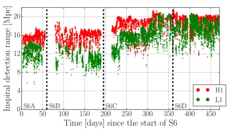
S6D S6B S6C S6A H1 L1Figure 4: The inspiral detection range of the LIGO detectors throughout S6 to a binary neutron star merger, averaged over sky location and orientation. The rapid improvements between epochs can be attributed to hardware and control changes implemented during commissioning periods.
thermal energy [32,33] – however, some of the observed limiting noise in this band was never understood. Above 150 Hz, shot noise due to variation in incident photon flux at the output port is the dominant fundamental noise source [34]. The sensitivity is also limited at many frequencies by narrow-band line structures, described in detail in section 4.7. The spectral sensitivity gives a time-averaged view of detector performance, and so is sensitive to the long-duration noise sources and signals, but rather insensitive to transient events.
A standard measure of a detector’s astrophysical reach is the distance to which that instrument could detect GW emission from the inspiral of a binary neutron star system with a signal-to-noise ratio (SNR) of 8 [35, 36], averaged over source sky locations and orientations. Figure4shows the evolution of this metric over the science run, with each data point representing an average over 2048 s of data. Over the course of the run, the detection range of H1 increased from∼16 to ∼20 Mpc, and of L1 from ∼14 to ∼20 Mpc. The instability of S6B at L1 can be seen between days 80–190, with a lower duty factor (also seen in table1) and low detection range; this period included extensive commissioning of the seismic feed-forward system at LLO [31].
The combination of increased amplitude sensitivity and improved duty factor over the course of S6 meant that the searchable volume of the universe for an astrophysical analysis was greatly increased.
4. Data-quality problems in S6
While the previous section described the performance of the LIGO detectors over the full span of the S6 science run, there were a number of isolated problems that had detrimental effects on the performance of each of the observatories at some time. Each of these problems, some of which are detailed below, introduced excess noise at specific times or frequencies that hindered astrophysical searches over the data.
Under ideal conditions, all excess noise sources can be quickly identified in the experimental set-up and corrected, either with a hardware change, or a modification of the control system. However, not all such fixes can be implemented immediately, or at all, and so noisy periods in auxiliary data (other data streams not directly associated with gravitational-wave readout) must be noted and recorded as likely to adversely affect the GW data. During S6, these data quality (DQ) flags and their associated time segments were used by analysis groups to inform decisions on which data to analyse, or which detection candidates to reject as likely noise artefacts, the impact of which will be discussed in section5.
The remainder of this section details a representative set of specific issues that were present for some time during S6 at LHO or LLO, some of which were fixed at the source, some which were identified but could not be fixed, and one which was never identified.
4.1. Seismic noise
Throughout the first-generation LIGO experiment, the impact of seismic noise was a fundamental limit to the sensitivity to GWs below 40 Hz. However, throughout S6 (and earlier science runs), seismic noise was also observed to be strongly correlated with transient noise glitches in the detector output, not only at low frequencies, but also at much higher frequencies (∼100-200 Hz).
The top panels of fig.5show the seismic ground motion at LHO, both in specific frequency bands (left) and as seen by the Ω-pipeline transient search algorithm [37] (right) - this panel shows localised seismic noise events in time and frequency coloured by their SNR. The lower left and right panels show transient events in the gravitational-wave strain data as recorded by single-interferomter burst and CBC inspiral searches respectively. Critically, during periods of high seismic noise, the inspiral analysis ‘daily ihope’ [13] produced candidate event triggers across the full range of signal templates, severely limiting the sensitivity of that search.
While great efforts were made to reduce the coupling of seismic noise into the interferometer [31], additional efforts were required to improve the identification of loud transient seismic events that were likely to couple into the GW readout [38]. Such times were recorded and used by astrophysical search groups to veto candidate events from analyses, proving highly effective in reducing the noise background of such searches.
4.2. Seismically-driven length-sensing glitches
While transient seismic noise was a problem throughout the science run, during late 2009 the presence of such noise proved critically disruptive at LLO. During S6B, the majority of glitches in L1 were correlated with noise in the length control signals of two short length degrees of freedom: the power recycling cavity length (PRCL), and the short Michelson formed by the beam-splitter and the input test masses (MICH). Both of these length controls were glitching simultaneously, and these glitches were correlated with more than 70% of the glitches in the GW data.
It was discovered that high microseismic noise was driving large instabilities in the power recycling cavity that caused significant drops in the circulating power, resulting in large glitches in both the MICH and PRC length controls. These actuation signals, applied to the main interferometer optics, then coupled into the detector output.
0 2 4 6 8 10 12 14 16 18 20 22 24 0.01 0.1 1 10
F
requency
[Hz]
0.5 11 5 10 10Normalized
ground
motion
0 2 4 6 8 10 12 14 16 18 20 22 24 100 103F
requency
[Hz]
5 10 10 50Signal-to-noise
ratio
(SNR)
5 10 15 20 25Binary
total
mass
[M
]
5 10 10 50Signal-to-noise
ratio
(SNR)
0 2 4 6 8 10 12 14 16 18 20 22 24Hour of August 19 2010 (UTC)
Science modeFigure 5: Seismic motion of the laboratory floor at LHO (normalized, top) and its correlation into GW burst (middle) and inspiral (bottom) analyses.
3pm 6pm 9pm 12am 3am 6am 9am 12pm 3pm 14 16 18 20 Inspiral range [Mp c]
3pm 6pm 9pm 12am 3am 6am 9am 12pm 3pm Local time [hours]
10−7 10−6 10−5 1-3 Hz ground motion [m/s]
Figure 6: Sensitive distance to a binary neutron star (top) and ground motion in the 1–3 Hz band (bottom) for a day at LLO. The inverse relationship is believed to be due to non-linear upconversion of low frequency seismic ground motions to higher frequency (∼40 − 200 Hz) noise in the GW output.
This issue was eliminated via commissioning of a seismic feed-forward system [31] that decreased the PRC optic motion by a factor of three. The glitchy data before the fix were identified by both the HierarchichalVeto (HVeto) and Used Percentage Veto (UPV) algorithms [39,40] – used to rank auxiliary signals according to the statistical significance of glitch coincidence with the GW data – with those times used by the searches to dismiss noise artefacts from their results (more in section5).
4.3. Upconversion of low-frequency noise due to the Barkhausen effect
In earlier science runs, as well as affecting performance below 40 Hz, increased levels of ground motion below 10 Hz had been associated with increases in noise in the 40– 200 Hz band. This noise, termed seismic upconversion noise, was produced by passing trucks, distant construction activities, seasonal increases in water flow over dams, high wind, and earthquakes [41, 21, 15,38]. During S6, this noise was often the limiting noise source at these higher frequencies. Figure6 shows a reduction in the sensitive range to binary neutron star (BNS) inspirals, contemporaneous with the workday increase in anthropogenic seismic noise.
Experiments subsequently showed that seismic upconversion noise levels correlated better with the amplitudes of the currents to the electromagnets that held the test masses in place as the ground moved than with the actual motion of the test masses or of the ground. An empirical, frequency-dependent function was developed to estimate upconversion noise from the low-frequency test mass actuation currents. This function was used to produce flags that indicated time periods that were expected to have high levels of seismic upconversion noise.
In addition to average reductions in sensitivity, upconverted seismic noise transients further reduced sensitivity to unmodelled GW bursts. Figure 7 shows that the rate of low-SNR glitches in the GW data – in a frequency band above
0
1
2
3
4
5
6
7
8
Weighted LHO coil current [RMS
×10
−22]
0
10
20
30
40
50
Num
b
er
of
glitc
hes
11
10
10
100
100
10
310
310
410
4Num
b
er
of
data
sections
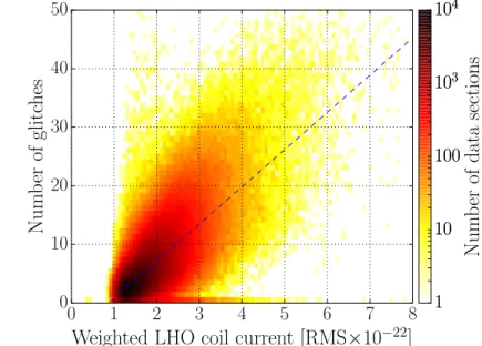
Figure 7: Correlation between low SNR glitches in the GW data, and current in the
test mass coil at H1. The r2 value measures the normalized cross-correlation
through a least-squares fit. This correlation is indicative of the Barkhausen effect.
that expected from linear seismic noise coupling – was correlated with the test mass actuation current, suggesting that seismic upconversion was the source of a low-SNR noise background that limited GW burst detection.
Investigations found that seismic upconversion noise bursts were clustered in periods of high slope in the amplitude of the magnetic actuator current. This was evidence that the seismic upconversion noise was Barkhausen noise [42]: magnetic field fluctuations produced by avalanches of magnetic domains in ferromagnetic materials that occur when the domains align with changing magnetic fields. The Barkhausen noise hypothesis was supported by investigations in which the noise spectrum was reproduced by magnetic fields that were generated independently of the system.
These investigations also suggested that the putative source of the Barkhausen noise was near or inside the test mass actuators. It was originally thought that the source of this upconversion noise was Barkhausen noise from NbFeB magnets, but a swap to less noisy SmCo magnets did not significantly reduce the noise [43]. However, it was found that fasteners inside the magnetic actuator, made of grade 303 steel, were ferromagnetic, probably because they were shaped or cut when cold. For aLIGO, grade 316 steel, which is much less ferromagnetic after cold working, is being used at the most sensitive locations.
4.4. Beam jitter noise
As described previously, one of the upgrades installed prior to S6 was the output mode cleaner, a bow-tie-shaped cavity designed to filter out higher-order modes of the main laser beam before detection at the output photodiode. As known from previous
experiments at GEO600 [44], the mode transmission of this cavity is very sensitive to angular fluctuations of the incident beam, whereby misalignment of the beam would cause non-linear power fluctuations of the transmitted light [45,46].
At LIGO, low-frequency seismic noise and vibrations of optical tables were observed to mix with higher-frequency beam jitter on the OMC to produce noise sidebands around the main jitter frequency. The amplitude of these sidebands was unstable, changing with the amount of alignment offset, resulting in transient noise at these frequencies, the most sensitive region of the LIGO spectrum, as seen in fig. 5 (bottom left panel). Mitigation of these glitches involved modifications of the suspension system for the auxiliary optics steering the beam into the OMC, to minimise the coupling of optical table motion to beam motion. Additionally, several other methods were used to mitigate and control beam jitter noise throughout the run: full details are given in [46].
4.5. Mechanical glitching at the reflected port
While the problems described up to this point have been inherent to the design or construction of either interferometer, the following two issues were both caused by electronics failures associated with the LHO interferometer.
The first of these was produced by faults in the servo actuators used to stabilize the pointing of the beam at the reflected port of the interferometer. This position is used to sense light reflected from the PRC towards the input, and generate control signals to correct for arm-cavity motion. The resulting glitches coupled strongly into the gravitational-wave data at∼37 Hz and harmonics.
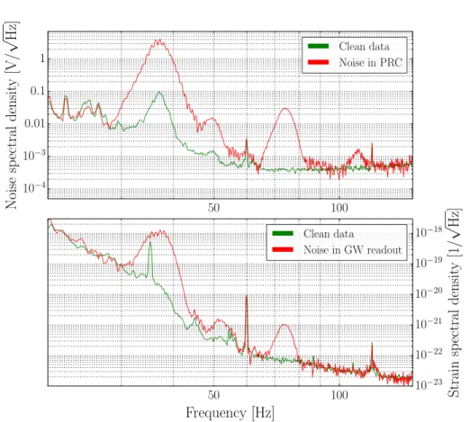
The source of the glitches was identified with the help of HVeto, which discovered that a number of angular and length sensing channels derived from photodiodes at the reflected port were strongly coupled with events in the GW data. Figure8shows the broad peaks in the spectra of one length sensing channel and the un-calibrated GW readout compared to a quiet reference time. On top of this, accelerometer signals from the optical table at the reflected port were found to be coupling strongly, having weak but coincident glitches.
These accelerometer coincidences indicated that the glitches were likely produced by mechanical motions of steering mirrors resulting from a faulty piezoelectric actuation system. Because of this, this servo was decomissioned for the rest of the run, leading to an overall improvement in data quality.
4.6. Broadband noise bursts from poor electrical connections
The second of the electronics problems caused repeated, broadband glitching in the LHO GW readout towards the end of S6. Periods of glitching would last from minutes to hours, and greatly reduced the instrumental sensitivity over a large frequency range, as shown in fig.9.
The main diagnostic clues were coincident, but louder, glitches in a set of quadrant photo-diodes (QPDs) sensing beam motion in the OMC. It was unlikely that these sensors could detect a glitch in the beam more sensitively than the GW readout photo-diode, and so the prime suspect then became the electronics involved with recording data from these QPDs.
In the process of isolating the cause, several other electronics boards in the output mode cleaner were inspected, re-soldered, and swapped for spares. The problem was
100 50 10−4 10−3 0.01 0.1 1
Noise
sp
ectral
densit
y
[V/
√
Hz]
Clean data Noise in PRC 100 50Frequency [Hz]
10−23 10−22 10−21 10−20 10−19 10−18Strain
sp
ectral
densit
y
[1/
√
Hz]
Clean data Noise in GW readoutFigure 8: Broad noise peaks centred at 37 Hz and its harmonics in the power recycling cavity length signal (top) and the GW output error signal (bottom). Each panel shows the spectrum as a noisy period (red) in comparison with a reference taken from clean data (green).
finally solved by re-soldering the connections on the electronics board that provided the high-voltage power supply to drive a piezoelectric transducer.
4.7. Spectral lines
Just as searches for transient signals are limited by instrumental glitches, so too our searches for steady signals are limited by a number of instrumental narrow-band peaks representing specific frequencies at which noise was elevated for a significant amount of time, in many cases for the entire science run. Many spectral lines are fundamental to the design and operation of the observatories, including alternating current (AC) power lines from the U.S. mains supply, at 60 Hz; violin modes from core-optic suspensions, around 350 Hz; and various calibration lines used to measure the interferometer response function.
Each of these features can be seen in fig.3at their fundamental frequency and a number of harmonics; however, also seen are a large number of lines from unintended sources, such as magnetic and vibrational couplings. These noise lines can have a damaging effect on any search for GWs if the frequencies of the incoming signal and of
100 103
F
requency
[Hz]
5 10 10 50Signal-to-noise
ratio
(SNR)
0 6 12 18 24 30 36 42 48 54 60 66 72Hours since midnight July 16 2010 (UTC)
Science mode
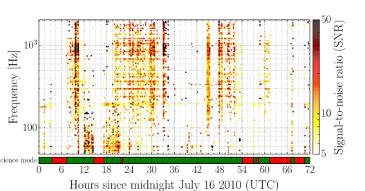
Figure 9: Noise events in the GW strain data recorded by the Ω-pipeline over a 60-hour period at LHO. The high SNR events above 100 Hz in hours 7–10, 20-34, and 44-42, were caused by broadband noise from a faulty electrical connection. The grid-like nature of these events is due to the discrete tiling in frequency by the trigger generator.
the lines overlap for any time; this is especially troublesome for searches for continuous gravitational-wave emitters.
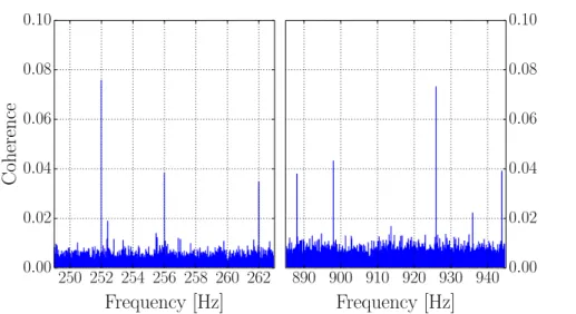
Throughout S6, series of lines were seen at both observatories as 2 Hz and 16 Hz harmonics. Figure 10 shows two separate groups of peaks in these harmonic sets found in coherence between the GW data for L1 and a magnetometer located near the output photo-detector. These lines were a serious concern for both the CW and SGWB searches due to their appearance at both observatories [47], leading to contamination of the coincidence-based searches for CW sources. Commissioning work on the OMC control system at LHO in early 2010 suggested that the use of a specific set of high-frequency (> 1 kHz) dither signals resulted in low-frequency noise generated by the digital-to-analog converters (DACs), but although resulting modifications to the controls scheme removed the 2 Hz series at that site, this hypothesis was never confirmed.
A number of other lines were isolated at either observatory site [47], and while not discussed in detail here, the cumulative effect of all spectral lines on searches for long-duration gravitational-wave sources is discussed in detail in section5.
4.8. The ‘spike’ glitch
The spike glitch was the name given to a class of very loud transients seen in the L1 instrument. They were characterized by a distinctive shape in the time series of the signal on the GW output photodiode, beginning with a rapid but smooth dip (lasting ∼1 ms) before a period of damped oscillation lasting ∼3 milliseconds, as shown in Figure 11. The amplitude of these glitches was extremely large, often visible in the raw time-series (which is normally dominated by low-frequency seismic motion), with the Ω-pipeline typically resolving these events with SNRs ranging from 200 to well
250 252 254 256 258 260 262
Frequency [Hz]
0.00 0.02 0.04 0.06 0.08 0.10Coherence
890 900 910 920 930 940Frequency [Hz]
0.00 0.02 0.04 0.06 0.08 0.10Figure 10: The coherence between the L1 GW readout signal and data from a magnetometer in the central building at LLO over one week of March 2010. 2 Hz and 16 Hz harmonics were seen to be coherent at numerous locations across the operating band of both interferometers, affecting the sensitivity of long-duration GW searches.
over 20,000.
The size and rapidity of the initial glitch suggested that the source was after the beams had re-combined at the beam-splitter before detection at the readout photodiode. The damped oscillations after the initial dip, however, were likely due to the response of the length control loop of the interferometer, meaning an actual or apparent sudden dip in the light on the output photodiode could explain the entire shape of the spike glitch. To investigate this possibility, the interferometer was run in a configuration where the light did not enter the arm cavities, but went almost directly into the OMC, removing the length and angular control servos from consideration. Sharp downward dips in the light were seen during this test, although they were 0.2 milliseconds wide, much narrower than the initial dips of the spike glitches.
Despite this investigation and many others, the cause of the spike glitch was never determined. However, these glitches were clearly not of astrophysical origin, and were not coherent with similar events in H1, allowing the CBC signal search to excise them from analyses by vetoing time around glitches detected in L1 with unreasonably high SNR. For future science runs, Advanced LIGO will consist of almost entirely new hardware, so whether the spike glitch or something very similar will be seen in new data remains to be seen.
5. The impact of data quality on gravitational wave searches
The impact of non-Gaussian, non-stationary noise in the LIGO detectors on searches for GWs is significant. Such loud glitches, such as the spike glitch, can mask or greatly disrupt transient GW signals present in the data at the same time, while high rates of lower SNR glitches can significantly increase the background in searches for these sources. Additionally, spectral lines and continued glitching in a given frequency range
-5 -4 -3 -2 -1 0 1 2 3 4 5
Time [seconds]
−6 −4 −2 0 2 4 6 ×10⁻¹⁷ -0.01 -0.005 0 0.005Time [seconds]
−6 −4 −2 0 2Gra
vitational-w
av
e
strain
Figure 11: A spike glitch in the raw GW photodiode signal for L1. The top panel shows the glitch in context with 10 s of data, while the bottom shows the glitch profile as described in the text.
reduces the sensitivity of searches for long-duration signals at those frequencies. Both long- and short-duration noise sources have a notable effect on search sensitivity if not mitigated.
Non-Gaussian noise in the detector outputs that can be correlated with auxiliary signals that have negligible sensitivity to GWs can be used to create flags for noisy data; these flags can then be used in astrophysical searches to remove artefacts and improve sensitivity. With transient noise, the flags are used to identify time segments in which the data may contain glitches. Similarly, spectral lines are recorded as frequencies, or narrow frequency bands, at which the detector sensitivity is reduced.
5.1. Data quality vetoes for transient searches
In this section, the impact of noisy data is measured by its effect on the primary analyses of the LIGO-Virgo transient search groups [4,7]:
• the low-mass CBC search ‘ihope’ [13] is a coincidence-based analysis in which data from each detector are filtered against a bank of binary inspiral template signals, producing an SNR time-series for each. Peaks in SNR across multiple detectors are considered coincident if the separation in time and matched template masses are small [48]. This analysis also uses a χ2-statistic test to down-rank signals
with high SNR but a spectral shape significantly different to that of the matched template [49].
• the all-sky cWB algorithm [10] calculates a multi-detector statistic by clustering time-frequency pixels with significant energy that are coherent across the detector network.
In both cases, the multi-detector events identified are then subject to a number of consistency tests before being considered detection candidates.
The background of each search is determined by relatively shifting the data from multiple detectors in time. These time shifts are much greater than the time taken for
Absolute deadtime % (seconds) Search deadtime % (seconds)
Instrument cWB ihope cWB ihope
H1 0.3% (53318) 0.4% (176079) 0.4% (77617) 3.8% (786284) L1 0.4% (75016) 0.1% (20915) 0.7% (137115) 6.2% (1180976)
Table 2: Summary of the reduction in all time and analysable time by category 1 veto segments during S6
a GW to travel between sites, ensuring that any multi-detector events in these data cannot have been produced by a single astrophysical signal.
Although both searches require signal power in at least two detectors, strong glitches in a single detector coupled with Gaussian noise in others still contributed significantly to the search background during S6. DQ flags were highly effective in removing these noise artefacts from the analyses. The effect of a time-domain DQ flag can be described by its deadtime, the fraction of analysis time that has been vetoed; and its efficiency, the fractional number of GW candidate events removed by a veto in the corresponding deadtime.
Flag performances are determined by their efficiency-to-deadtime ratio (EDR); random flagging and vetoing of data gives EDR '1, whereas effective removal of glitches gives a much higher value. Additionally, the used percentage – the fraction of auxiliary channel glitches which coincide with a GW candidate event – allows a measure of the strength of the correlation between the auxiliary and GW channel data.
Each search group chose to apply a unique set of DQ flags in order to minimise deadtime whilst maximising search sensitivity; for example, the CBC search teams did not use a number of flags correlated with very short, high-frequency disturbances, as these do not trigger their search algorithm, while these flags were used in searches for unmodelled GW bursts.
We present the effect of three categories of veto on each of the above searches in terms of reduction in analysable time and removal of noise artefacts from the search backgrounds. Only brief category definitions are given, for full descriptions see [15].
5.1.1. Category 1 vetoes. The most egregious interferometer performance problems are flagged as category 1. These flags denote times during data taking when the instrument was not running under the designed configuration, and so should not be included in any analysis.
The Data Monitoring Tool (DMT) automatically identified certain problems in real time, including losses of cavity resonance, and errors in the h(t) calibration. Additionally, scientists monitoring detector operation in the control room at each observatory manually flagged individual time segments that contained observed instrumental issues and errors.
All LIGO-Virgo search groups used category 1 vetoes to omit unusable segments of data; as a result their primary effect was in the reduction in analysable time over which searches were performed. This impact is magnified by search requirements on the duration for analysed segments, with the cWB and ihope searches requiring a minimum of 316 and 2064 seconds of contiguous data respectively. Table2outlines the absolute deadtime (fraction of science-quality data removed) and the search deadtime (fractional reduction in analysable time after category 1 vetoes and segment selection).
At both sites the amount of science-quality time flagged as category 1 is less than half of one percent, highlighting the stability of the instrument and its calibration. However, the deadtime introduced by segment selection is significantly higher, especially for the CBC analysis. The long segment duration requirement imposed by the ihope pipeline results in an order of magnitude increase in search deadtime relative to absolute deadtime.
5.1.2. Categories 2 and 3. The higher category flags were used to identify likely noise artefacts. Category 2 veto segments were generated from auxiliary data whose correlation with the GW readout has been firmly demonstrated by instrumental commissioning and investigations. Category 3 includes veto segments from less well understood statistical correlations between noisy data in an auxiliary channel and the GW readout. Both the ihope and cWB search pipelines produce a first set of candidate event triggers after application of category 2 vetoes, and a reduced set after application of category 3.
The majority of category 2 veto segments were generated in low-latency by the DMT and include things like photodiode saturations, digital overflows, and high seismic and other environmental noise. At category 3, the HVeto [39], UPV [40], and bilinear-coupling veto (BCV) [50] algorithms were used, by the burst and CBC analyses respectively, to identify coupling between auxiliary data and the GW readout. Table3gives the absolute, relative, and cumulative deadtimes of these categories after applying category 1 vetoes and segment selection criteria, outlining the amount of analysed time during which event triggers were removed. As with category 1, category 2 vetoes have deadtimeO(1)%, but with significantly higher application at L1 compared to H1. This is largely due to one flag vetoing the final 30 seconds before a lock-loss combined with the relative abundance of short data-taking segments for L1. Additionally, photodiode saturations and computational timing errors were more prevalent at the LLO site than at LHO and so contribute to higher relative deadtime. Category 3 flags contributedO(10)% deadtime for each instrument. While this level of deadtime is relatively high, as we shall see, the efficiency of these flags in removing background noise events makes such cuts acceptable to the search groups.
H1 L1
Deadtime type Cat. cWB ihope cWB ihope
Absolute % (s) 2 0.26% 0.77% 1.59% 1.53% 3 7.90% 9.26% 8.54% 7.03% Relative % (s) 3 7.73% 9.00% 7.06% 6.10% Cumulative % (s) 3 7.97% 9.71% 8.54% 7.54%
Table 3: Summary of the absolute, relative, and cumulative deadtimes introduced
by category 2 and 3 veto segments during S6. The relative deadtime is
the additional time removed by category 3 not vetoed by category 2, and cumulative deadtime gives the total time removed from the analysis.
Figure12shows the effect of category 3 vetoes on the background events from the cWB pipeline; these events were identified in the background from time time-slides and are plotted using the SNR reconstructed at each detector. This search applies category 2 vetoes in memory, and does not record any events before this step, so efficiency statements are only available for category 3. The results are shown after
![Figure 1: Optical layout of the LIGO interferometers during S6 [21]. The layout differs from that used in S5 with the addition of the output mode cleaner.](https://thumb-eu.123doks.com/thumbv2/123doknet/14249501.488009/10.918.152.694.127.509/figure-optical-layout-interferometers-layout-differs-addition-cleaner.webp)