HAL Id: hal-00938738
https://hal-enac.archives-ouvertes.fr/hal-00938738
Submitted on 29 Apr 2014HAL is a multi-disciplinary open access
archive for the deposit and dissemination of sci-entific research documents, whether they are pub-lished or not. The documents may come from teaching and research institutions in France or abroad, or from public or private research centers.
L’archive ouverte pluridisciplinaire HAL, est destinée au dépôt et à la diffusion de documents scientifiques de niveau recherche, publiés ou non, émanant des établissements d’enseignement et de recherche français ou étrangers, des laboratoires publics ou privés.
control
Antoine Drouin, Alexandre Carlos Brandao-Ramos, Thierry Miquel, Felix
Mora-Camino
To cite this version:
Antoine Drouin, Alexandre Carlos Brandao-Ramos, Thierry Miquel, Felix Mora-Camino. Rotorcraft trajectory tracking by non linear inverse control. DINCON 2007, 6th Brazilian Conference on Dynam-ics, Control and their Applications, May 2007, São José do Rio Preto, Brazil. pp xxxx. �hal-00938738�
Rotorcraft Trajectory Tracking by Non Linear Inverse Control
Antoine Drouin
LARA and UAV Research Unit at ENAC, Toulouse, France
[email protected] Alexandre Brandão Ramos
Instituto de Ciências Exatas, UNIFEI, Itajubá, Brazil
[email protected] Thierry Miquel
DSNA/DTI/DGAC and LARA/ENAC, Toulouse, France
[email protected] Félix Mora-Camino
LARA/ENAC and LAAS du CNRS, Toulouse, France
Abstract:
The purpose of this communication is to investigate the usefulness of the non linear inverse control approach to solve the trajectory tracking problem for a four rotor aircraft. After introducing simplifying assumptions, the flight dynamics equations for the four rotor aircraft are considered. A trajectory tracking control structure based on a two layer non linear inverse approach is then proposed.A supervision level is introduced to take into account the actuator limitations.Keywords:
Rotorcraft flight mechanics, nonlinear inverse control, trajectory tracking.1.INTRODUCTION
In the last years a large interest has risen for the four rotor concept since it appears to present simultaneously hovering, orientation and trajectory tracking capabilities of interest in many practical applications [1].
The flight mechanics of rotorcraft are highly non linear and different control approaches (integral LQR techniques, integral sliding mode control [2], reinforcement learning [3]) have been considered with little success to achieve not only autonomous hovering and orientation, but also trajectory tracking In this paper, after introducing some simplifying assumptions, the flight dynamics equations for a four rotor aircraft with fixed pitch blades are considered.
The purpose of this study is to investigate the usefulness of the non linear inverse control approach to solve the trajectory tracking problem for this class of rotorcraft. This approach has been already considered in the case of aircraft trajectory tracking by different authors [4,5,6].
It appears that the flight dynamics of the considered rotorcraft present a two level input affine structure which is made apparent when a new set of equivalent inputs is defined. This allows to introduce a non linear inverse control approach with two time scales, one devoted to attitude control and one devoted to orientation and trajectory tracking.
Rotor dynamics are discussed in annex 1 and since the control approach does not take into account explicitly the limitations of the actuators, a supervision layer is also proposed.
2. ROTORCRAFT FLIGHT DYNAMICS
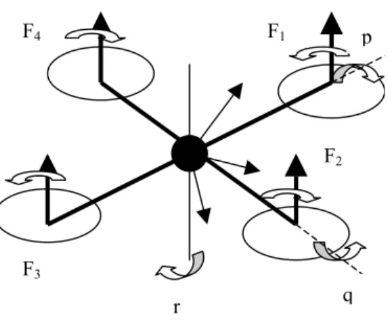
The considered system is shown in figure 1 where rotors one and three are clockwise while rotors two and four are counter clockwise. Annex 1 describes the rotor dynamics.
The main simplifying assumptions adopted with respect to flight dynamics in this study are a rigid cross structure, no wind, negligible aerodynamic contributions resulting from translational speed, no ground effect as well as negligible air density effects and very small rotor response times. It is then possible to write simplified rotorcraft flight equations [7].
Figure 1- Four rotor aircraft
The moment equations can be written as:
) ( ) / ( ) ( ) / ( ) ( ) / ( 3 4 1 2 4 3 1 2 2 4 F F F F I k r r p k F F I a q r q k F F I a p zz yy xx − + − = + − = + − = & & & (1)
where p, q, r are the components of the body angular
velocity, with and
xx yy zz I I
I
k2( − )/ k4=(Ixx−Izz)/Iyy,
Ixx, Iyy and Izz being the moments of inertia in body-axis
and m the total mass of the rotorcraft. The Euler equations are given by:
r q r q r q p )) cos( / ) (cos( )) cos( / ) ((sin( ) sin( ) cos( ) cos( ) tan( ) sin( ) tan( θ φ θ φ ψθ φ φ φ θ φ θ φ + = − = + + = & & & (2)
where θ, φ, and ψ are respectively the pitch, bank and
heading angles.
The acceleration equations written directly in the local Earth reference system are such as:
F M g z F m y F m x ) cos( ) cos( ) / 1 ( )) sin( ) cos( ) cos( ) sin( ) )(sin( / 1 ( )) sin( ) sin( ) cos( ) sin( ) )(cos( / 1 ( φ θθ φ ψ φ ψψ θ φ ψ φ + − == − + = & & & & & & (3)
where x, y and z are the centre of gravity coordinates
and where : (4) 4 3 2 1 F F F F F = + + +
and with the constraints:
{
1,2,3,40≤F ≤Fmax i∈
i
i
}
(5)3. NLI FLIGHT CONTROL APPROACH
Here we are interested in controlling the four rotor aircraft so that its centre of gravity follows a given
path with a given heading ψ while attitude angles θ
and φ remain small. Many potential applications
require not only the centre of gravity of the device to follow a given trajectory but also the aircraft to present a given orientation.
F4 F1 p
3.1 Attitude control
F2
From equations (1) it appears that the
effectiveness of the rotor actuators is much larger with respect to the roll and pitch axis than with respect to the yaw axis. Then we consider that attitude control is
involved with controlling the θ and φ angles. In
equations (1) the effect of rotor forces appears as
differences so, we define new attitude inputs u1 and u2
as: F3 q r 3 1 1 F F u = −
u
2=
F
2−
F
4 (6.1)In the heading and position dynamics, the effects of rotor forces and moments appear as sums, so we
define new guidance inputs v1 and v2 as:
3 1
1
F
F
v
=
+
v
2=
F
2+
F
4 (6.2)It is supposed that u1 and u2 can be made to vary
significantly while v1 and v2 can remain constant.
Then the attitude dynamics can be rewritten under the affine input form:
U X g V X f X&= ( , )+ ( ) (7.1) Y'=(θ,φ) (7.2) with ) , , , ( ' p qθ φ X = , U'=(u1,u2) andV'=(v1,v2) (8)
Then, considering the non linear inverse control theory, it appears that the attitude angles present relative degrees equal to one and that there is no internal dynamics while the output equations can be rewritten as: ) ( ) ( ) (Y U N X V P X M Y&&= + + (9) with ⎥ ⎦ ⎤ ⎢ ⎣ ⎡ − = cossin/ / 0/ ) ( yy xx yy I a I a I tg a Y M
φ
φ
θ
(10) ⎥⎦ ⎤ ⎢⎣ ⎡ − − = zz zz zz I tg k I tg k I k I k X N / cos / cos / sin / sin ) ( φ θ φ θ φ φ (11) ]' , [ ) (X P1 P2 P = where: )) cos sin ( ( ) cos sin ( cos 4 1 φ θ φ θ φ φ r p tg φq rtg q r p k P + + + − = (12.1)dt tg d r dt tg d q tg r p k r q k P / ) cos ( / ) sin ( sin 4 2 2 φ θ φ θ φ θ + + + = (2.2)
It appears that while φ≠±π/2, the attitude dynamics
given by (9) are invertible. Then it appears feasible to consider as control objective to get second order linear attitude dynamics towards reference values:
⎥
⎥
⎦
⎤
⎢
⎢
⎣
⎡
−
−
−
−
−
−
=
=
⎥
⎦
⎤
⎢
⎣
⎡
)
(
2
)
(
2
2 2 c c d d dY
φ
φ
ω
φ
ω
ζ
ω
θ
ω
θ
θ
ζ
φ
θ
φ φ φ θ θ θ&
&
&
&
&
&
&
&
(13)where
ζ
θ,ζ
φ,ω
θ,ω
φ are respectively damping andnatural frequency parameters while θc and φc are
reference values for the attitude angles.
Then the corresponding non linear inverse attitude control law is given by:
) ) ( ) ( ( ) (X 1 N X V P X Yd M U =− − + −&& (14)
3.2 Design of a guidance control law
Considering that the attitude dynamics are stable and faster than the guidance dynamics, the guidance equations can be approximated by the control affine form: ⎥ ⎥ ⎥ ⎥ ⎥ ⎥ ⎦ ⎤ ⎢ ⎢ ⎢ ⎢ ⎢ ⎢ ⎣ ⎡ + + − − + + + − = ⎥ ⎥ ⎥ ⎥ ⎥ ⎦ ⎤ ⎢ ⎢ ⎢ ⎢ ⎢ ⎣ ⎡ ) ( ) cos( ) cos( ) / 1 ( ) ( )) sin( ) cos( ) cos( ) sin( ) )(sin( / 1 ( ) ( )) sin( ) sin( ) cos( ) sin( ) )(cos( / 1 ( ) ( cos cos 2 1 2 1 2 1 1 2 v v m g v v m v v m v v I k z y x c c c c c c c c c zz c φ θ ψ φ φ θ ψψ θ φ ψ φ θ φ ψ & & & & & & & & (15)
Here also, the outputs of the guidance dynamics present relative degrees equal to 1 while the internal dynamics, which are concerned with the attitude angles , are supposed already stabilized. Then, supposing that second order linear dynamics are of interest for the guidance variables, we can define desired accelerations by: ⎥ ⎥ ⎥ ⎥ ⎥ ⎦ ⎤ ⎢ ⎢ ⎢ ⎢ ⎢ ⎣ ⎡ − − − − − − − − − − − − = ⎥ ⎥ ⎥ ⎥ ⎦ ⎤ ⎢ ⎢ ⎢ ⎢ ⎣ ⎡ ) ( 2 ) ( 2 ) ( 2 ) ( 2 2 2 2 2 c z z z c y y y c x x x c c c c c z z z y y y x x x z y x ω ω ζ ω ω ζζ ω ω ψ ψ ω ψ ω ζ ψ ψ ψ ψ & & & & & & & & & & & & (16)
where ζψ,ζx,ζy,ζz,ωψ,ωx,ωy,ωzare respectively
damping and natural frequency parameters while ψc,
xc, yc and zc are reference values for the attitude
angles. Of course, many other schemes can be proposed to define desired accelerations at the guidance level.
Once desired accelerations are made available, the inversion of the guidance dynamics brings nominal the solution: ) cos cos ) ( ( 2 1 2 2 2 1 c c c zz c c c k I g z y x m v ψ φθ && & & & & & & + + + − = (17.1) ) cos cos ) ( ( 2 1 2 2 2 2 c c c zz c c c k I g z y x m v ψ φθ && & & & & & & + + + + = (17.2) with )) /( ) sin cos ((x y z g arctg c c c
c= && ψ+&& ψ && +
θ (18.1) and 2 2 2 ) ( cos sin arcsin( g z y x y x d d d d c c + + + − = & & & & & & & & & &
ψ
ψ
φ
(18.2) p, q, θ, φψ
,
x
,
y
,
z
Figure 2-Proposed control structure
Then, returning to the expression of the attitude control law , it happens that the centre of gravity acceleration terms compensate each others and the law becomes:
) ) ( ) ( ( ) ( 1 d Y X P X N X M U=− − + −&& (19) with c c c c c N N X N ψ φφ θ θ θ φφ θ & & ⎥ ⎥ ⎥ ⎥ ⎦ ⎤ ⎢ ⎢ ⎢ ⎢ ⎣ ⎡ − = ⎥ ⎦ ⎤ ⎢ ⎣ ⎡ = cos cos cos cos sin cos sin cos ) ( 2 1 (20) Attitude dynamics Guidance dynamics NLI attitude control NLI guidance control c c c c &x& &y& z&&
& & , , , ψ z y x z y x
r,ψ&,&,&,&, , ,
θc,φc u1,u2 v1 ,v2, θc, φc θ, φ Attitude control loop Guidance control loop
The whole proposed control structure is given in the above figure 2.
4. FLIGHT CONTROL SUPERVISION
Since the above control approach does not consider explicitly the input level constraints, we introduce here a supervision layer whose function is to avoid the generation of unfeasible reference values for the inputs by modifying, as less as possible, the current control objectives. According to (5), (6) and (7), the control signals should be such as:
2 , 1 max max≤ ≤ = −F ui F i (21.1) and 0≤vi ≤2Fmax i=1,2 (21.2)
Conditions (21.1) implies for the desired attitude accelerations to satisfy the following conditions:
max
min
φ
φ
φ
&& ≤ && ≤ &&c (22.1) with max 2 2 min cos F I a P N yy φ φ&& = + − (22.2) and max 2 2 max cos F I a P N yy φ φ&& = + + (22.3) and condition: max min θ θφ θ
θ&& ≤ && − && ≤ &&
c c tg (23.1) with ) ( ) ( / 1 1 2 2 max min =−aF Ixx+ N +P −tgθ N +P θ&& (23.2) and ) ( ) ( / 1 1 2 2 max max =aF Ixx+ N +P −tgθ N +P θ&& (23.3)
Then, reference v alues for instant attitude angles
accelerations can be obtained from the solution of the following linear –quadratic optimization problem:
2 2 ( ) ) ( min θ α φ β β αr c− + c− & & & & (24.1) with max min
β
φ
φ
&& ≤ ≤ && (24.2)max
min α θ β θ
θ&& ≤ −tg ≤&& (24.3)
Observe that the solution of this problem is equal to (θ& ,&c φ&&c) if it is feasible with respect to constraints (24.2) and (24.3), otherwise the solution will be on the border of the convex feasible set.
Then if α*and β*are solution of this problem, u
1 and
u2 are given by:
) ) ( ) ( ( ) ( * * 1 2 1 ⎥ ⎦ ⎤ ⎢ ⎣ ⎡ − + − = ⎥ ⎦ ⎤ ⎢ ⎣ ⎡ − β α X P V X N X M u u (25)
In the case of v1 and v2 (relations (21.2)) and
considering the expressions of θc and φc the above
approach leads to the consideration of an intricate non convex optimization problem. A different approach is
proposed here. Let λ be such as:
) ( ,
,y y z g z g
x
x&r = &&c &&r= &&c &&r+ = &&c+
& λ λ λ (26)
then according to (18.1) and (18.2):
c r θ
θ = and φ =r φc (27)
Feasible reference values for
x&
&
r,&
y&
r,&
z&
r andψ
&
&
rcanbe obtained from the solution of the following linear – quadratic optimization problem:
2 2 2 , ( 1) ( ) min λ η μ ψc μ λ − + −&& (28.1) with max 2 2 2 4 ) cos cos ( ) ) ( ( 0 F k I g z y x m c c zz c c c + + + − ≤
≤ && && && λ φθ μ (28.2) max 2 2 2 4 ) cos cos ( ) ) ( ( 0 F k I g z y x m c c zz c c c + + + + ≤
≤ && && && λ φθ μ (28.3)
where η is here a time constant. Let and be
the solution of the above problem, then the control inputs can be taken as:
* λ μ* ) cos cos ) ( ( 2 1 * 2 2 2 * 1 μ φθ λ c c zz c c c k I g z y x m
v = && +&& + && + − (29.1) ) cos cos ) ( ( 2 1 * 2 2 2 * 2 λ φθ μ c c zz c c c k I g z y x m
v = && +&& + && + + (29.2) Then: 2 / ) ( 1 1 1 u v F = + F2 =(u2 +v2)/2 (30.1) 2 / ) ( 1 1 3 v u F = − F4=(v2 −u2)/2 (30.1)
5. CASE STUDIES
Here we consider two cases: one where the objective is to hover at an initial position of
coordinates x0, y0, z0 while acquiring a new orientation
ψ1, and one where the rotorcraft is tracking the
helicoïdal trajectory of equations:
t t xc()=ρcosν t t yc()=ρsinν t zc=δ+γ (31) 2 / ) ( ν π ψc t = t+
where ρ is a constant radius and γ is a constant path
5.1 Heading control at hover
In this case we get the guidance control laws:
) ( 2 1 1 zz c k I g m v = − ψ&& ( ) 2 1 2 zz c k I g m v = + ψ&& (32)
with the following reference values for the attitude angles:
0 =
c
θ and φc=0 (33)
Here the heading acceleration is given by:
) ( 2 1 2ψ ψ ω ω ζ ψ&&c =− ψ ψr− ψ − (34)
Starting from an horizontal attitude ( θ(0)=0, φ(0)=0),
attitude inputs u1 and u2 given by relation (14) remain
equal to zero. Then, figures 3 and 4 display some simulation results:
00 0 . 5 1 1 . 5 2 2 . 5 3 3 . 5 4 4 . 5 5
5 1 0 1 5
Figure 3-Hover control inputs
00 0 . 5 1 1 . 5 2 2 . 5 3 3 . 5 4 4 . 5 5 0 . 2 0 . 4 0 . 6 0 . 8 1 1 . 2 1 . 4 1 . 6
Figure 4-Heading response during hover
5.2 Trajectory tracking case
In this case we get the guidance control laws:
) ( 2 1 2 2 2 2 1 v m g v = = ρν + (38)
Here the permanent reference values for the attitude angles are such as:
0 = c θ (39.1) and 2 4 2 2 sin g c + − = ν ρ ν ρ φ (39.2)
and the desired guidance and orientation accelerations are given by:
0 , 0 ) sin( 2 = = − = c c c z t y ψ ν ν ρ & & & & & & (40) Attitude inputs are given by relation (14) where now:
⎥ ⎦ ⎤ ⎢ ⎣ ⎡ − = − ) /( ) /( 1 ) cos /( 0 1 xx xx yy I a tg tg I a a I M φ θ φ (41) and
[
0 0 )' (X = N]
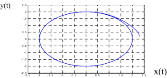
(41)In figures 5 to 7 simulation results are displayed where at initial time the rotorcraft is hovering:
y(t) -2 . 5 -2 -1 . 5 -1 -0 . 5 0 0 . 5 1 1 . 5 2 2 . 5 -2 . 5 -2 -1 . 5 -1 -0 . 5 0 0 . 5 1 1 . 5 2 2 . 5 F1,F3 x(t)
Figure 5- Evolution of rotorcraft horizontal track
F2,F4 time 0 0 . 5 1 1 . 5 2 2 . 5 3 3 . 5 4 4 . 5 5 0 0 . 0 2 0 . 0 4 0 . 0 6 0 . 0 8 0 . 1 0 . 1 2 0 . 1 4 z(t) ψ-ψc time
Figure 6- Evolution of rotorcraft altitude
time 0 0.5 1 1.5 2 2.5 3 3.5 4 4.5 5 0 2 4 6 8 10 12 14 F2,F4 F1 F3 time
Figure 7- Rotorcraft trajectory tracking inputs
6. CONCLUSIONS
In this communication the theoretical applicability of the non linear inverse control technique to rotorcraft trajectory tracking has been investigated. It appears that this approach leads to the design of a two level control structure based on analytical laws.
Considering the structure of the rotorcraft flight dynamics, other promising non linear control techniques are differential flat control [8] and back stepping control [9].
When considering the complexity of these non linear control laws involving a relatively small number of inputs, neural networks components could be of interest for their effective implementation.
However, the robustness of these control laws with respect to the different aerodynamic effects which have been taken as negligible should be investigated. Since only very intricate theories are available to approach this problem, real flight tests appear, at this stage, to be unavoidable.
REFERENCES
[1] Hoffmann, G., Rajnarayan, D.G., Waslander, S. L., Dostal , D., Jang, J.S. and Tomlin, C. J., The
Standford Tetsbed of Autonomous Rotorcraft for Multi-Agent Control, 23rd Digital Avionics Systems Conference, Salt Lake City, UT, November 2004. [2] Hassan K. Khalil, Nonlinear Systems, Prentice
Hall, 3rd Ed., 2002.
[3] Sutton R.S. and Barto, A. G., Reinforcement
learning: an introduction, MIT Press, Cambridge,
MA, 1998.
[4] Singh, S. N. and Schy, A. A., Nonlinear decoupled
control synthesis for maneuvring aircraft,
Proceedings of the 1978 IEEE conference on Decision and Control, Piscataway, NJ, 1978. [5] Ghosh, R. and Tomlin,C. J., Nonlinear Inverse
Dynamic Control for Model-based Flight,
Proceeding of AIAA, 2000.
[6] Asep, R., Shen, T.J., Achaíbou, K. and Mora-Camino, F., An application of the nonlinear inverse
technique to flight-path supervision and control,
Proceedings of the 9th International Conference of Systems Engineering, Las Vegas,NV, 1993. [7] Etkin, B. and Reid L. R., Dynamics of
Flight-Stability and Control. John Wiley & Sons. New
York, NY, 1996.
[8] Lu, W.C., Mora-Camino, F. and Achaibou, K. ,
Flight Mechanics and Differential Flatness.
Dincon 04, Proceedings of Dynamics and Control Conference, Ilha Solteira, Brazil, pp. 830-839, 2004.
[9] Miquel, T., Contribution à la synthèse de lois de
guidage relatif, approche non linéaire. PhD.
Thesis, Université Paul Sabatier, Toulouse, 2004.
Annex 1.
The rotor engine dynamics are characterized by the
relation between the input voltage Va and the angular
rate ω. A possible model of rotor dynamics is given by:
) ( ) / ( ) ( ) ( 1 ) (t τω t KQω t 2 KVa τ Va t ω& =− − + (A.1)
with ω =(0) ω0 , where τ , KQ and KVa are given
positive parameters and where the voltage input is such as:
max
0≤Va ≤V (A.2)
with a negligible time response for the voltage generator.
The step response (Va =constant) of the rotor is
solution of the scalar Riccati equation:
a V Q t K V K t t) 1 () () ( a/ ) ( ω ω 2 τ τ ω& =− − + (A.3) with ω(0)=ω0 .
A particular solution ω1 of the associated differential
equation is such as: ( 1 4 1) 2 1 1= + V Q a− Q V K K K a τ τ ω (A.4)
In the general case, the solution of (A.3) can be written as ' / ' / 1 1 ) 1 ( ' ) 0 ( 1 1 ) ( τ τ τ ω ω ω ω t t Q e e K t − − − + − + = (A.5) with (A.6) a Q VK V K τ τ τ'= / 1+4 and (A.7) 1 ) ( limω =ω +∞ → t t 0 .1 .2 .3 .4 .5 .6 .7 .8 .9 1 1.5 2 2.5
Omega (rad/s) Va=2
0 .1 .2 .3 .4 .5 .6 .7 .8 .9 . 1 0
5 10 15
omega (rad/s) Va=20
Figure 8- Two examples of rotor step response
It appears from figure 8 that the dynamics of the rotor may be close to those of a first order linear system with
time constant τ’, but as can be seen in (A.6), this value
is a function of Va.
If the desired dynamics for the output are such as:
1( )
c
T ω ω
ω&=− − (A.8)
where T is a very small time constant Va can be chosen
such as: ) ) ( ) ( ) 1 (( 1 ) ( 2 t K T t T K t V c Q V a a ω τ ω τ ω τ + + − = (A.9)
The rotor forces are then given by: 4 1 2 to i f Fi = ωi = (A.10)
4 1 to i F k Mi = i = (A.11)