HAL Id: hal-03154036
https://hal.archives-ouvertes.fr/hal-03154036
Submitted on 26 Feb 2021
HAL is a multi-disciplinary open access
archive for the deposit and dissemination of
sci-entific research documents, whether they are
pub-lished or not. The documents may come from
teaching and research institutions in France or
abroad, or from public or private research centers.
L’archive ouverte pluridisciplinaire HAL, est
destinée au dépôt et à la diffusion de documents
scientifiques de niveau recherche, publiés ou non,
émanant des établissements d’enseignement et de
recherche français ou étrangers, des laboratoires
publics ou privés.
two-dimensional leap-frog scheme: approximation and
fast implementation
Christophe Besse, Jean-François Coulombel, Pascal Noble
To cite this version:
Christophe Besse, Jean-François Coulombel, Pascal Noble.
Discrete transparent boundary
conditions for the two-dimensional leap-frog scheme:
approximation and fast implementation.
ESAIM: Mathematical Modelling and Numerical Analysis, EDP Sciences, 2021, 55, pp.S535-S571.
�10.1051/m2an/2020052�. �hal-03154036�
https://doi.org/10.1051/m2an/2020052 www.esaim-m2an.org
DISCRETE TRANSPARENT BOUNDARY CONDITIONS FOR THE
TWO-DIMENSIONAL LEAP-FROG SCHEME: APPROXIMATION AND FAST
IMPLEMENTATION
Christophe Besse
1,*, Jean-Franc
¸ois Coulombel
1and Pascal Noble
2Abstract. We develop a general strategy in order to implement approximate discrete transparent boundary conditions for finite difference approximations of the two-dimensional transport equation. The computational domain is a rectangle equipped with a Cartesian grid. For the two-dimensional leap-frog scheme, we explain why our strategy provides with explicit numerical boundary conditions on the four sides of the rectangle and why it does not require prescribing any condition at the four corners of the computational domain. The stability of the numerical boundary condition on each side of the rectangle is analyzed by means of the so-called normal mode analysis. Numerical investigations for the full problem on the rectangle show that strong instabilities may occur when coupling stable strategies on each side of the rectangle. Other coupling strategies yield promising results.
Mathematics Subject Classification. 65M06, 65M12.
Received September 6, 2019. Accepted July 25, 2020.
1. Introduction
In this article, we are concerned with the construction and numerical implementation of discrete transparent boundary conditions for linear transport equations. Our goal is to derive numerical boundary conditions that minimize the parasitic wave reflections at the boundary of the computational domain. This research area has been increasingly active since the pioneering work by Engquist and Majda [19] and our goal here is to explain why following the same “small frequency approximation” strategy as in [19] can be successful at the fully discrete level when one deals with a rectangular computational domain. Namely, we shall construct fully discrete, approximate transparent boundary conditions for the two-dimensional leap-frog scheme on a rectangle. Our numerical boundary conditions will not be exactly transparent since the derivation of such conditions on a rectangle seems to be out of reach. Our strategy is to start from the exact transparent boundary conditions for a half-space and, as in [19], to localize them with respect to the tangential variable by means of a suitable “small frequency approximation”. This general strategy may be applied to any finite difference scheme. In terms of wave reflection magnitude, our numerical simulations show that our approximate transparent boundary conditions
Keywords and phrases. Transport equation, leap-frog schemes, transparent boundary conditions, stability.
1 Institut de Math´ematiques de Toulouse, UMR5219, Universit´e de Toulouse, CNRS, Universit´e Paul Sabatier,
F-31062 Toulouse Cedex 9, France.
2 Institut de Math´ematiques de Toulouse, UMR5219, Universit´e de Toulouse, CNRS, INSA, F-31077 Toulouse, France. *Corresponding author: [email protected]
c
○ The authors. Published by EDP Sciences, SMAI 2021
This is an Open Access article distributed under the terms of theCreative Commons Attribution License(https://creativecommons.org/licenses/by/4.0), which permits unrestricted use, distribution, and reproduction in any medium, provided the original work is properly cited.
are more efficient than more standard, purely local extrapolation strategies, hence, in our opinion, the relevance of implementing discrete time convolution operators as described below.
We focus here on the discretization of the two-dimensional transport equation by means of the leap-frog scheme. The nice feature of this approximation is that it does not dissipate high frequency signals – and therefore allows for a precise analysis of wave reflections on each side of the rectangle – and, moreover, its stencil exhibits some “dimensional splitting”. The latter feature will be helpful in our construction since we shall not have to develop a specific numerical treatment for the four corners of the computational domain. Hence we shall focus on the numerical boundary conditions on each of the four sides of the rectangle and on their coupling through the eight mesh points that are closest to the four corners. More simple, purely local, outflow strategies [1,21,24,35] may be implemented for dissipative schemes (e.g., the Lax–Wendroff scheme). Even though these extrapolation boundary conditions are much cheaper from a computational point of view and are quite efficient in terms of absence of wave reflection for dissipative schemes, they only give poor intuition for more complex wave propagation phenomena modeled for instance by the Schr¨odinger or Airy equations. Moreover, our simulations clearly show that local extrapolation boundary conditions for the leap-frog scheme give rise to larger reflected waves than those generated by the boundary conditions we shall construct below. For inflow boundaries, high order local numerical treatments based on the inverse Lax–Wendroff method [16,20,31,33,36] have also been constructed and analyzed in the past. As for extrapolation strategies at outflow boundaries, these numerical treatments may yield good convergence properties. However, they generate wave reflections whose magnitude is larger than what we observe with our nonlocal (in time) procedure. Despite a more involved implementation and a higher computational cost, we thus believe that nonlocal strategies as those examined below may be relevant.
An alternative strategy to the one developed below would consist in starting from the exact transparent boundary condition for the underlying partial differential equation (the continuous problem) and then trying to discretize it. This strategy has been examined, at least, in [2,8,23], and the overall conclusion is that there is no general answer for the construction of such absorbing boundary conditions if one wishes to maintain stability. We therefore rather follow the approach developed in [3,18] and later used in a wide variety of contexts, and thus construct (approximate) transparent boundary conditions that are adapted to the considered finite difference approximation.
Exact Discrete Transparent Boundary Conditions (DTBC in what follows) are analytically available in two space dimensions only when the computational domain is a half-space (Z𝑑−1× N) or the product of a half-line by a torus ((Z/𝐽 Z)𝑑−1× N). By “analytically available”, we mean that DTBC can be expressed by a well-defined operator, even though its practical implementation may be difficult. We refer for instance to [2–4,15] and references therein for various aspects of the theory, the main features of which are recalled below. In either case, the discrete spatial domain is a cylinder of the form 𝒟 × N with no tangential boundary (the variables in 𝒟) so DTBC can be derived by performing either a Fourier transform or a Fourier series decomposition with respect to the spatial tangential variables. In the end, this approach yields a one-dimensional problem that is parametrized by the tangential frequency1. In that framework, the two-dimensional DTBC thus take the form of a tangential pseudo-differential operator that is intrinsically nonlocal. In order to be implemented on a rectangular computational domain, one therefore has to make the DTBC local, which we achieve here as in [19] by using a suitable “small frequency approximation”, which is meaningful (at least formally) for smooth solutions. The frequency cut-off amounts to retaining only finitely many terms in the Taylor expansion of the symbol of the DTBC operator and rewriting the Taylor expansion as a trigonometric polynomial (up to higher order terms). This cut-off strategy is implemented here in such a way that the stencil used for the numerical boundary conditions is not wider than that of the interior numerical scheme. Higher order strategies could be relevant but would require a specific treatment when getting closer to the corner. We do not investigate this issue here.
As in all numerical approximation problems, a crucial feature for the efficiency of the numerical scheme is stability. Following the general result of [15], the DTBC for the leap-frog scheme on a half-space do not meet the strongest possible stability properties because the leap-frog scheme exhibits glancing wave packets (even in one space dimension). On a half-space, the exact DTBC meet some kind of neutral stability which calls for special care since a slight modification in the numerical boundary conditions may yield violent instabilities. In what follows, we show that the zero, first and second order tangential frequency cut-off – as described above – maintain neutral stability when implemented on a half-space (the so-called Godunov–Ryabenkii condition is satisfied [22]). In other words, our approximate transparent boundary conditions are as spectrally stable as the exact ones on a half-space and we therefore feel rather safe to implement them on a rectangular geometry. If instabilities occur in the rectangular geometry, they will necessarily stem from the coupling between the various numerical boundary conditions on each side of the rectangle. A thorough stability analysis on the rectangle seems to be out of reach at the present time. It is not even fully understood at the continuous level! The numerical investigations that we report below show that stability in the rectangle should not be taken for granted. Some coupling strategies exhibit good stability – and convergence – properties while at least one displays violent instabilities. In a future work, we shall extend our strategy to fully discretized hyperbolic systems and to implicit difference schemes for dispersive equations.
Let us now give the plan of our work. In Section 2, we introduce the two-dimensional transport equation and the leap-frog scheme on a rectangular computational domain. The goal is then to construct and analyze approximate transparent boundary conditions. For later use and also for the ease of reading, we first go back to the corresponding one-dimensional problem in Section3. We adapt the general strategy of [3,18], which was recently generalized in [15], to the particular case of the leap-frog scheme. Some of the tools used in [15] are complemented here by some explicit expansions, based on Legendre polynomials, which were already used in [3,12,18]. Such explicit representation formulae lower the implementation cost of our method and give a sharp asymptotic behavior for the convolution coefficients, which would not be possible by only using the tools in [15]. We then analyze the stability of the one-dimensional DTBC by means of the normal mode decomposition and show that they satisfy the so-called Godunov–Ryabenkii condition [22]. Since the numerical implementation and computational cost of DTBC is sometimes considered as heavy, we then discuss the fast implementation of approximate DTBC by the so-called sum of exponential approach. We relax some of the constraints used in [3,18] for the free parameters in this approximation, and show that the resulting approximation is efficient from a numerical cost point of view and also from the wave reflection magnitude point of view. Section4extends this approach to the two-dimensional problem by first considering the exact DTBC on a half-space and then using low frequency truncations in order to derive local (in the tangential space variable) approximate DTBC. We analyze, for the half-space problem, the stability of our approximate DTBC and then report on some numerical simulations on the rectangle.
2. The transport equation and the leap-frog approximation
In this article, we consider the linear advection equation in two space dimensions: {︂ 𝜕𝑡𝑢 + c · ∇𝑢 = 0, 𝑡 ≥ 0, (𝑥, 𝑦) ∈ R2,
𝑢|𝑡=0= 𝑢0,
(2.1)
where the space coordinates are denoted (𝑥, 𝑦), the velocity reads c = (𝑐𝑥, 𝑐𝑦)𝑇 and ∇ = (𝜕𝑥, 𝜕𝑦)𝑇. It is always assumed from now on that the velocity c is nonzero. To fix ideas, we shall always take 𝑐𝑥 and 𝑐𝑦 to be nonnegative, but this has no impact on the analysis below. The solution to (2.1) reads:
𝑢(𝑡, 𝑥, 𝑦) = 𝑢0(𝑥 − 𝑐𝑥𝑡, 𝑦 − 𝑐𝑦𝑡),
so if the initial condition 𝑢0 is supported, say in the square [−𝐿, 𝐿] × [−𝐿, 𝐿], the solution vanishes in the larger square [−2𝐿, 2𝐿] × [−2𝐿, 2𝐿] after some time 𝑇 ∼ 𝐿/|c|. Given a finite difference approximation to (2.1)
associated with a Cartesian grid, our goal in this article is to propose a systematic construction of transparent, or approximate transparent numerical boundary conditions2 in order to simulate the advection of the initial condition through the computational domain and eventually its exit through the numerical boundary. Our goal is to minimize as much as possible parasitic wave reflections on the numerical boundary.
In all what follows, the computational domain is a fixed rectangle [𝑥ℓ, 𝑥𝑟] × [𝑦𝑏, 𝑦𝑡] (ℓ, 𝑟, 𝑏, 𝑡 stand for left, right, bottom and top). We consider some space steps 𝛿𝑥, 𝛿𝑦 > 0 such that the ratios:
𝑥𝑟− 𝑥ℓ
𝛿𝑥 =: 𝐽 + 1,
𝑦𝑡− 𝑦𝑏
𝛿𝑦 =: 𝐾 + 1,
define some integers 𝐽 and 𝐾 (that are meant to be large). Eventually, the time step 𝛿𝑡 > 0 will always be chosen so that the parameters
𝜇𝑥 := 𝑐𝑥 𝛿𝑡
𝛿𝑥, 𝜇𝑦 := 𝑐𝑦 𝛿𝑡 𝛿𝑦,
are fixed (or at worse vary between two fixed positive constants). These parameters should satisfy some stability requirement, the so-called Courant–Friedrichs–Lewy condition, as explained below. The grid points are defined as (𝑥𝑗, 𝑦𝑘), with:
∀ 𝑗 = 0, . . . , 𝐽 + 1, ∀ 𝑘 = 0, . . . , 𝐾 + 1, 𝑥𝑗 := 𝑥ℓ+ 𝑗 𝛿𝑥, 𝑦𝑘 := 𝑦𝑏+ 𝑘 𝛿𝑦.
The interior points correspond to 1 ≤ 𝑗 ≤ 𝐽 and 1 ≤ 𝑘 ≤ 𝐾. The four sides of the rectangle (the numerical boundary) correspond to 𝑗 ∈ {0, 𝐽 + 1} and 𝑘 ∈ {0, 𝐾 + 1}.
Letting now 𝑢𝑛𝑗,𝑘 denote the approximation of the exact solution to (2.1) at (𝑥𝑗, 𝑦𝑘) and time 𝑛 𝛿𝑡, the two-dimensional leap-frog scheme reads:
𝑢𝑛+2𝑗,𝑘 − 𝑢𝑛 𝑗,𝑘+ 𝜇𝑥(︀𝑢𝑛+1𝑗+1,𝑘− 𝑢 𝑛+1 𝑗−1,𝑘)︀ + 𝜇𝑦(︀𝑢𝑛+1𝑗,𝑘+1− 𝑢 𝑛+1 𝑗,𝑘−1 )︀ = 0, (2.2)
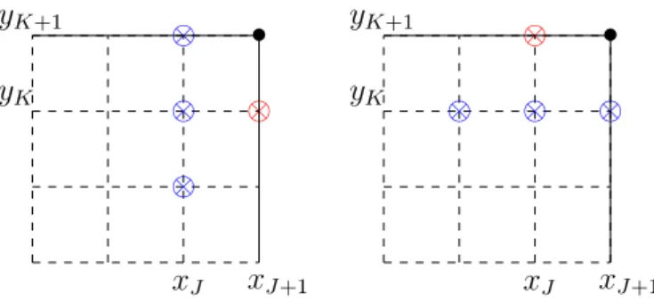
which holds for 1 ≤ 𝑗 ≤ 𝐽 and 1 ≤ 𝑘 ≤ 𝐾, that is at all interior points. The definition of the numerical scheme requires to prescribe numerical boundary conditions for 𝑢𝑛+20,𝑘 , 𝑢𝑛+2𝐽 +1,𝑘, 𝑘 = 1, . . . , 𝐾, and 𝑢𝑛+2𝑗,0 , 𝑢𝑛+2𝑗,𝐾+1, 𝑗 = 1, . . . , 𝐽 . A crucial observation for what follows is that the update of the numerical solution in the interior does not require to prescribe any numerical boundary condition at the corners (this is because 𝑢𝑛+2𝑗,𝑘 does not depend on 𝑢𝜎𝑗±1,𝑘±1 at any earlier time index 𝜎). In all what follows, the numerical solution (𝑢𝑛𝑗,𝑘) will therefore be defined for (𝑗, 𝑘) ∈ {0, . . . , 𝐽 + 1} × {0, . . . , 𝐾 + 1} ∖ {(0, 0), (0, 𝐾 + 1), (𝐽 + 1, 0), (𝐽 + 1, 𝐾 + 1)}. We shall be careful in our definition of the numerical boundary conditions to make sure that the four corner values are not involved either.
Let us note that on the whole space Z2, the ℓ2-stability condition for (2.2) reads:
𝜇𝑥+ 𝜇𝑦≤ cfl < 1, (2.3) where cfl is a free positive parameter to be chosen. We consider the case 𝑐𝑥, 𝑐𝑦 ≥ 0, hence 𝜇𝑥, 𝜇𝑦 ≥ 0, so we do not write absolute values in (2.3). The inequality (2.3) gives an upper bound for 𝛿𝑡 in terms of 𝛿𝑥, 𝛿𝑦. The bound (2.3), or its one-dimensional analogue that we shall discuss below, is always assumed to hold from now on.
We wish to construct approximate transparent boundary conditions for (2.2) on each side of the rectangle. For ease of reading and also for future use on the two-dimensional problem (2.2), we first go back to the one-dimensional problem and briefly recall the construction of DTBC for the one-one-dimensional leap-frog scheme. We discuss the various possible implementations of the DTBC and approximations by means of sums of exponentials. This technique was used for instance in [3] in the context of the Schr¨odinger equation and later extended to other contexts. Once the tools have been set in one space dimension, we shall feel free to use them in two space dimensions whenever it makes sense.
3. Discrete transparent boundary conditions for the one-dimensional
leap-frog scheme
3.1. The numerical scheme
We now consider the one-dimensional transport equation:
{︂ 𝜕𝑡𝑢 + 𝑐𝑥𝜕𝑥𝑢 = 0, 𝑡 ≥ 0, 𝑥 ∈ R,
𝑢|𝑡=0= 𝑢0, (3.1)
with an initial condition 𝑢0that is supported in an interval [𝑥ℓ; 𝑥𝑟]. For concreteness, we shall assume from now on 𝑐𝑥> 0 so that the initial condition is transported towards the right and eventually exits the initial support [𝑥ℓ; 𝑥𝑟]. We are interested here in simulating the solution to (3.1) on the fixed interval [𝑥ℓ; 𝑥𝑟] by imposing suitable non-reflecting boundary conditions at the boundary points 𝑥ℓ, 𝑥𝑟.
As in the previous section, we choose a mesh size 𝛿𝑥 > 0 such that 𝑥𝑟− 𝑥ℓ
𝛿𝑥 =: 𝐽 + 1,
is an integer. The time step 𝛿𝑡 > 0 is chosen in such a way that the parameter 𝜇𝑥 defined by: 𝜇𝑥 := 𝑐𝑥
𝛿𝑡 𝛿𝑥,
is a fixed positive constant. Keeping the notation 𝑥𝑗 := 𝑥ℓ+ 𝑗 𝛿𝑥, 𝑗 = 0, . . . , 𝐽 + 1, and letting now 𝑢𝑛𝑗 denote the approximation of the solution to (3.1) at 𝑥𝑗 and time 𝑛 𝛿𝑡, the one-dimensional leap-frog scheme reads
𝑢𝑛+2𝑗 − 𝑢𝑛
𝑗 + 𝜇𝑥(︀𝑢𝑛+1𝑗+1− 𝑢 𝑛+1
𝑗−1)︀ = 0, 𝑗 = 1, . . . , 𝐽. (3.2) The parameter 𝜇𝑥 is fixed by imposing:
𝜇𝑥≤ cfl < 1, (3.3)
which is a necessary and sufficient ℓ2 stability requirement for (3.2
) on the whole real line 𝑗 ∈ Z, see [22,29]. Since 𝜇𝑥 is positive in our framework, we thus fix 𝜇𝑥∈ (0, 1) and let 𝛿𝑥, 𝛿𝑡 vary accordingly.
The numerical sheme (3.2) on the interval 1 ≤ 𝑗 ≤ 𝐽 requires a definition for the boundary values 𝑢𝑛+10 , 𝑢𝑛+1𝐽 +1, and a definition for the initial data (𝑢0𝑗), (𝑢1𝑗). The initial condition (𝑢0𝑗) is defined by setting
∀ 𝑗 = 0, . . . , 𝐽 + 1, 𝑢0𝑗 := 𝑢0(𝑥𝑗),
where 𝑢0 is the initial condition for (3.1). In the numerical simulations reported below, we have chosen [𝑥ℓ, 𝑥𝑟] = [−3, 3] and 𝑢0(𝑥) = exp(−10 𝑥2). The first time step value (𝑢1𝑗) is defined by imposing the second order Lax–Wendroff scheme in the interior domain, namely:
∀ 𝑗 = 1, . . . , 𝐽, 𝑢1𝑗 := 𝑢0𝑗−𝜇𝑥 2 (𝑢 0 𝑗+1− 𝑢 0 𝑗−1) + 𝜇2 𝑥 2 (𝑢 0 𝑗+1− 2 𝑢 0 𝑗+ 𝑢 0 𝑗−1).
The boundary values 𝑢10 and 𝑢1𝐽 +1 are set equal to zero for simplicity (which is almost exact for the Gaussian initial condition that we consider). We now recall how to derive the DTBC for the scheme (3.2).
3.2. Derivation of DTBC
The goal of this paragraph is to derive the DTBC for the leap-frog scheme (3.2). We follow the methodology of [18], which was originally designed for the Schr¨odinger equations, and therefore consider the numerical scheme:
𝑢𝑛+2𝑗 − 𝑢𝑛𝑗 + 𝜇𝑥(︀𝑢𝑛+1𝑗+1− 𝑢 𝑛+1
on the whole real line Z, assuming that the initial conditions (𝑢0
𝑗)𝑗∈Z, (𝑢1𝑗)𝑗∈Zbelong to ℓ2and vanish outside of the interval {1, . . . , 𝐽 }. The stability condition (3.3) is assumed to hold. The DTBC are first computed in terms of the so-called 𝒵-transform of the sequences (𝑢𝑛
𝑗)𝑛∈N. Let us briefly recall the definition of the 𝒵-transform (we do not pay too much attention here to the convergence of the Laurent series involved in the computations below and rather remain at the level of formal series).
Definition 3.1. Let (𝑢𝑛)𝑛∈N∈ CNbe a sequence. The 𝒵-transform of (𝑢𝑛)𝑛∈N, which is denoted̂︀𝑢, is defined by:
̂︀ 𝑢(𝑧) := ∞ ∑︁ 𝑛=0 𝑢𝑛 𝑧𝑛,
the series being well-defined and holomorphic in {𝑧 ∈ C, |𝑧| > 𝑅} where 1/𝑅 is the convergence radius of ∑︀∞
𝑛=0𝑢𝑛𝑤
𝑛 (here 𝑤 is a placeholder for 1/𝑧 and the radius 𝑅 may be zero or infinite). We now let ˆ𝑢𝑗(𝑧), 𝑗 ∈ Z, denote the 𝒵-transform of the sequence (𝑢𝑛𝑗)𝑛∈N:
ˆ 𝑢𝑗(𝑧) := ∞ ∑︁ 𝑛=0 𝑢𝑛𝑗 𝑧−𝑛.
It is shown in [15] that the above series converges for |𝑧| > 1 thanks to the ℓ2-stability of the leap-frog scheme3.
Moreover, the sequence (ˆ𝑢𝑗(𝑧))𝑗∈Zis square integrable. We apply the 𝒵-transform to the numerical scheme (3.4) and obtain:
(︀𝑧 − 𝑧−1)︀ ˆ𝑢
𝑗+ 𝜇𝑥(︀ ˆ𝑢𝑗+1− ˆ𝑢𝑗−1 )︀
= 0, (3.5)
for 𝑗 ≤ 0 and 𝑗 ≥ 𝐽 + 1. (On the interval {1, . . . , 𝐽 }, the initial conditions give rise to a nonzero source term on the right hand side of (3.5).) The equation (3.5) is a recurrence relation and we therefore look for the solutions to the characteristic equation:
𝜅2+𝑧 − 𝑧 −1
𝜇𝑥
𝜅 − 1 = 0. (3.6)
The two roots to (3.6) are given by
𝜅± :=
𝑧−1− 𝑧 ±√︀𝑧2+ 2 (2 𝜇2
𝑥− 1) + 𝑧−2 2 𝜇𝑥
, (3.7)
with the standard definition of the square root (the branch cut is R−). When |𝑧| → +∞, |𝜅
−| → +∞ and |𝜅+| → 0. Moreover, 𝜅± do not belong to S1 for |𝑧| > 1 so we have |𝜅+| < 1 and |𝜅−| > 1 for |𝑧| > 1. We thus relabel these two roots as a stable and unstable one and write from now on:
𝜅0𝑠(𝑧) := 𝑧 −1− 𝑧 +√︀𝑧2+ 2 (2 𝜇2 𝑥− 1) + 𝑧−2 2 𝜇𝑥 , 𝜅0𝑢(𝑧) := 𝑧 −1− 𝑧 −√︀𝑧2+ 2 (2 𝜇2 𝑥− 1) + 𝑧−2 2 𝜇𝑥 · (3.8) The reason for the superscript 0 will be clear in the next section when we deal with the two-dimensional problem. The recurrence relation (3.5) and the decay at infinity of (ˆ𝑢𝑗(𝑧))𝑗∈Z implies:
ˆ 𝑢𝐽 +1(𝑧) = 𝜅0𝑠(𝑧) ˆ𝑢𝐽(𝑧), 𝑢ˆ0(𝑧) = 1 𝜅0 𝑢(𝑧) ˆ 𝑢1(𝑧). (3.9)
It now remains to compute the Laurent series expansion of both 𝜅0
𝑠 and 1/𝜅0𝑢 and to perform the inverse 𝒵-transform in order to write the numerical boundary conditions (3.9) in the original discrete time variable 𝑛. Since we have 𝜅0𝑠(𝑧) 𝜅0𝑢(𝑧) = −1, see (3.6), we can equivalently rewrite (3.9) as:
ˆ
𝑢𝐽 +1(𝑧) = 𝜅0𝑠(𝑧) ˆ𝑢𝐽(𝑧), 𝑢ˆ0(𝑧) = −𝜅0𝑠(𝑧) ˆ𝑢1(𝑧). (3.10) 3This is where the condition 𝜇
There are at least two ways to compute the Laurent series expansion of 𝜅0
𝑠 for the leap-frog scheme, which we now detail in order to compare the possible benefits and drawbacks of each method. The first method is rather in the spirit of [18] while the second one follows [11,15].
An explicit expansion in terms of Legendre polynomials. The first method to obtain this expansion relies on the explicit formula (3.8) and on the expansion
1 √ 1 − 2 𝑥 𝑡 + 𝑡2 = ∞ ∑︁ 𝑛=0 𝑃𝑛(𝑥) 𝑡𝑛, (3.11)
where 𝑃𝑛 denotes the 𝑛th-Legendre polynomial [32]. This family of polynomials can be equivalently defined by the first two terms 𝑃0(𝑥) := 1, 𝑃1(𝑥) := 𝑥 and by the recurrence formula:
∀ 𝑛 ≥ 1, (𝑛 + 1) 𝑃𝑛+1(𝑥) := (2𝑛 + 1) 𝑥 𝑃𝑛(𝑥) − 𝑛 𝑃𝑛−1(𝑥). (3.12) Starting from (3.8), we have
√︀ 𝑧2+ 2 (2 𝜇2 𝑥− 1) + 𝑧−2= 𝑧 1 − 2 (1 − 2 𝜇2 𝑥) 𝑧−2+ 𝑧−4 √︀1 − 2 (1 − 2 𝜇2 𝑥) 𝑧−2+ 𝑧−4 = 𝑧 (1 − 2 𝛼𝑥𝑧−2+ 𝑧−4) ∞ ∑︁ 𝑛=0 𝑃𝑛(𝛼𝑥) 𝑧−2𝑛,
with 𝛼𝑥:= 1 − 2 𝜇2𝑥∈ (−1, 1). We therefore derive the expansion 2 𝜇𝑥𝑧 𝜅0𝑠(𝑧) = 1 − 𝑧 2+(︀𝑧2− 2 𝛼 𝑥+ 𝑧−2)︀ ∞ ∑︁ 𝑛=0 𝑃𝑛(𝛼𝑥) 𝑧−2𝑛. (3.13)
We focus below on the right boundary condition at point 𝑥𝐽 +1= 𝑥𝑟. Going back to (3.10) and using the above expansion (3.13) for 𝜅0 𝑠, the DTBC (3.10) reads 2 𝜇𝑥𝑧 ˆ𝑢𝐽 +1(𝑧) = (︃ 1 + ∞ ∑︁ 𝑛=0 𝐵𝑛𝑧−2𝑛 )︃ ˆ 𝑢𝐽(𝑧), with ∀ 𝑛 ∈ N, 𝐵𝑛 := 𝑃𝑛+1(𝛼𝑥) − 2 𝛼𝑥𝑃𝑛(𝛼𝑥) + 𝑃𝑛−1(𝛼𝑥),
and it is understood that 𝑃−1 vanishes (in the expression of 𝐵0). We compute 𝐵0 = −𝛼𝑥, and thanks to the recurrence relation (3.12), we get the shorter expression
∀ 𝑛 ≥ 1, 𝐵𝑛 = 𝑃𝑛−1(𝛼𝑥) − 𝑃𝑛+1(𝛼𝑥) 2 𝑛 + 1 , and finally 2 𝜇𝑥𝑧 ˆ𝑢𝐽 +1(𝑧) = (︃ 2 𝜇2𝑥+ ∞ ∑︁ 𝑛=1 𝑃𝑛−1(𝛼𝑥) − 𝑃𝑛+1(𝛼𝑥) 2 𝑛 + 1 𝑧 −2𝑛 )︃ ˆ 𝑢𝐽(𝑧). (3.14) Recall that in (3.14), we use the notation 𝛼𝑥= 1 − 2 𝜇2𝑥.
We now look for an efficient way to implement the coefficients of the above series without using the expression of the Legendre polynomials (which would be computationally rather cheap anyway). Let us define the sequence (𝑠0𝑛)𝑛≥0such that 𝑠00:= 𝜇𝑥, 𝑠01:= 𝜇𝑥(1 − 𝜇2𝑥), and 𝑠
0
𝑛 := (𝑃𝑛−1(𝛼𝑥) − 𝑃𝑛+1(𝛼𝑥))/((4 𝑛 + 2) 𝜇𝑥) for 𝑛 ≥ 2. After various simplifications using (3.12), we obtain
∀ 𝑛 ≥ 2, 𝑠0𝑛 = 2 𝑛 − 1 𝑛 + 1 (1 − 2 𝜇 2 𝑥) 𝑠 0 𝑛−1− 𝑛 − 2 𝑛 + 1𝑠 0 𝑛−2. (3.15)
The DTBC (3.14) therefore reads ˆ 𝑢𝐽 +1(𝑧) = ∞ ∑︁ 𝑛=0 𝑠0𝑛𝑧−2 𝑛−1𝑢ˆ𝐽(𝑧). (3.16) Performing the inverse 𝒵-transform, we get4:
𝑢𝑛+2𝐽 +1 = ∑︁ 0≤𝑚≤(𝑛+1)/2
𝑠0𝑚𝑢𝑛+1−2 𝑚𝐽 . (3.17)
The recurrence relation (3.15) may be efficiently implemented in a computer code, which gives access to the coefficients in the numerical boundary condition (3.17) up to any prescribed final time index 𝑁𝑓. Going back to (3.10), we also derive the “left” numerical boundary condition:
𝑢𝑛+20 = − ∑︁ 0≤𝑚≤(𝑛+1)/2
𝑠0𝑚𝑢𝑛+1−2 𝑚1 . (3.18)
In view of understanding the stability properties of the numerical boundary condition (3.18), it might be important to determine the asymptotics of the sequence (𝑠0
𝑛)𝑛∈N. Let us recall that 𝑠0𝑛 equals (𝑃𝑛−1(𝛼𝑥) − 𝑃𝑛+1(𝛼𝑥))/((4 𝑛 + 2) 𝜇𝑥) for 𝑛 ≥ 2 (here 𝜇𝑥∈ (0, 1) and 𝛼𝑥= 1 − 2 𝜇2𝑥). We use the so-called Laplace formula for the Legendre polynomials, see Theorem 8.21.2 of [32]:
∀ 𝜃 ∈ (0, 𝜋), 𝑃𝑛(cos 𝜃) = √︂ 2 𝜋 𝑛 sin 𝜃 cos (︂(︂ 𝑛 +1 2 )︂ 𝜃 −𝜋 4 )︂ + 𝑂(𝑛−3/2), (3.19) where the remainder term is even uniform with respect to 𝜃 on every compact set of the form [𝜀, 𝜋 − 𝜀], 𝜀 > 0. We fix the angle 𝜃𝑥 ∈ (0, 𝜋) such that cos 𝜃𝑥 = 𝛼𝑥 = 1 − 2 𝜇𝑥2, and therefore sin 𝜃𝑥 = 2 𝜇𝑥√︀1 − 𝜇2𝑥. We then apply the Laplace formula and obtain after a few simplifications:
𝑠0𝑛 = (1 − 𝜇 2 𝑥)1/4 √︀ 𝜋 𝜇𝑥𝑛3 sin (︂(︂ 𝑛 +1 2 )︂ 𝜃𝑥− 𝜋 4 )︂ + 𝑂(𝑛−5/2). (3.20) This asymptotic behavior can be verified on numerical experiments.
Determining inductively the expansion. As observed in [11,15], the Laurent series expansion of 𝜅0 𝑠 can also be computed inductively by using the equation (3.6). The main benefit is that the method does not rely on an explicit knowledge of a power series expansion such as the one involving the Legendre polynomials (which is useful only for three point schemes). The methodology below is therefore more flexible in view of being generalized to numerical schemes with larger stencils (as the one considered in [11]).
We know that 𝜅0𝑠 tends to zero at infinity so we may plug its Laurent series expansion5 ∑︀ 𝑛≥1𝜎 0 𝑛𝑧−𝑛 into (3.6) and obtain (︀𝑧 − 𝑧−1)︀ ∞ ∑︁ 𝑛=1 𝜎0𝑛𝑧−𝑛+ 𝜇𝑥 ⎛ ⎝ (︃∞ ∑︁ 𝑛=1 𝜎0𝑛𝑧−𝑛 )︃2 − 1 ⎞ ⎠ = 0, which is found to be equivalent to 𝜎0
1 = 𝜇𝑥 and ∀ 𝑛 ∈ N, 𝜎0𝑛+2= 𝜎𝑛0− 𝜇𝑥 𝑛 ∑︁ 𝑚=1 𝜎0𝑚𝜎0𝑛+1−𝑚, (3.21)
4It is understood in (3.17) that the summation holds over all integers 𝑚 between 0 and (𝑛 + 1)/2. In case 𝑛 is even, then the
summation holds over all integers 𝑚 between 0 and 𝑛/2.
5It is proved in [15] that the Laurent series is convergent for |𝑧| > 1 which follows from the splitting of the two roots of (3.6) for
where we use the convention 𝜎0
0= 0. It is not difficult to see that if 𝑛 is even, then 𝜎𝑛0= 0. Let now 𝑛 = 2 𝑝 + 1 be odd, 𝑝 ≥ 0. An easy computation gives
𝜎2 𝑝+30 = 𝜎02 𝑝+1− 𝜇𝑥 𝑝 ∑︁ 𝑚=0
𝜎2 𝑚+10 𝜎02(𝑝−𝑚)+1.
This means that the sequence (𝑠0
𝑛)𝑛∈Nappearing in (3.17) and that satisfies the recurrence relation (3.15) also satisfies 𝑠0𝑛+1 = 𝑠0𝑛− 𝜇𝑥 𝑛 ∑︁ 𝑝=0 𝑠0𝑝𝑠0𝑛−𝑝, (3.22) with 𝑠0
0 = 𝜇𝑥 (𝑠0𝑛 coincides with 𝜎2 𝑛+10 ). Observe that the value 𝑠01 = 𝜇𝑥(1 − 𝜇2𝑥) that we have found in the previous paragraph is consistent with (3.22). It seems less clear to derive the asymptotic behavior (3.20) by starting from (3.22) rather than from the more explicit representation (3.14). Both approaches thus seem to have their own interest.
Given the initial conditions (𝑢0𝑗)0≤𝑗≤𝐽 +1and (𝑢1𝑗)0≤𝑗≤𝐽 +1as described above (𝑢0is determined by the initial condition for the transport equation and 𝑢1 is determined by applying the Lax–Wendroff method), both of which satisfy 𝑢0
0= 𝑢10= 𝑢0𝐽 +1= 𝑢1𝐽 +1= 0, the leap-frog scheme on the interval {1, . . . , 𝐽 } with DTBC reads: 𝑢𝑛+2𝑗 = 𝑢𝑛𝑗 − 𝜇𝑥 (︀𝑢𝑛+1𝑗+1 − 𝑢 𝑛+1 𝑗−1)︀ , 1 ≤ 𝑗 ≤ 𝐽, 𝑛 ∈ N, (3.23a) 𝑢𝑛+20 = − ∑︁ 0≤𝑚≤(𝑛+1)/2 𝑠0𝑚𝑢𝑛+1−2 𝑚1 , (3.23b) 𝑢𝑛+2𝐽 +1= ∑︁ 0≤𝑚≤(𝑛+1)/2 𝑠0𝑚𝑢𝑛+1−2 𝑚𝐽 , (3.23c)
where the parameter 𝜇𝑥in (3.23) is fixed such that 0 ≤ 𝜇𝑥< 1 and the sequence (𝑠𝑛0)𝑛∈Nis defined by 𝑠00= 𝜇𝑥, 𝑠0
1 = 𝜇𝑥(1 − 𝜇2𝑥) and the recurrence relation (3.15) for 𝑛 ≥ 2 (or equivalently (3.22), but this is slightly less efficient from a numerical point of view). We recall that we consider the case 𝑐𝑥≥ 0 in (3.1), hence the sign for 𝜇𝑥, but the other case 𝑐𝑥≤ 0 can be dealt with the same arguments (assuming −1 < 𝜇𝑥≤ 0).
3.3. Stability analysis on a half-line
In this short paragraph, we explain why the normal mode analysis predicts “neutral stability” for any of the two half-line problems where the leap-frog scheme (3.23a) is considered on the half-line {𝑗 ≤ 𝐽 } or {𝑗 ≥ 1}, in combination with either (3.23b) or (3.23c). Let us focus on the case {𝑗 ≥ 1}, since the other case is entirely similar.
The normal mode analysis consists in determining the solutions of the leap-frog scheme (3.23a) of the form 𝑢𝑛
𝑗 = 𝑧𝑛𝑣𝑗, with |𝑧| > 1, and (𝑣𝑗) ∈ ℓ2. Among such sequences, the final question is to determine whether there exist nonzero ones that satisfy the numerical boundary condition (3.23b). Following [22], we shall say that the Godunov–Ryabenkii condition is satisfied if there is no nonzero sequence (𝑣𝑗) ∈ ℓ2 such that 𝑢𝑛𝑗 = 𝑧
𝑛𝑣 𝑗 is a solution to the leap-frog scheme that satisfies (3.23b). Otherwise, we shall say that 𝑧 is an unstable eigenvalue. Of course, unstable eigenvalues preclude (in the most violent way) stability estimates hence a desirable feature of any numerical boundary condition is to satisfy the Godunov–Ryabenkii condition.
Plugging the ansatz 𝑢𝑛𝑗 = 𝑧𝑛𝑣𝑗 in the leap-frog scheme, we find that the sequence (𝑣𝑗) should belong to ℓ2 and satisfy
∀ 𝑗 ≥ 1, (︀𝑧2− 1)︀ 𝑣
𝑗 + 𝜇𝑥𝑧(︀𝑣𝑗+1− 𝑣𝑗−1)︀ = 0.
The computation of the ℓ2-solutions to this recurrence relation follows by solving the characteristic equation (3.6) and by determining among the roots to (3.6) which have modulus less than 1. This classification has
already been performed in the previous paragraph, so for |𝑧| > 1, we can conclude that the sequence (𝑣𝑗) is given by
∀ 𝑗 ≥ 1, 𝑣𝑗 = 𝑣0𝜅0𝑠(𝑧) 𝑗, 𝑣
0∈ C.
Inserting into (3.23b), we have to determine whether among such sequences (that are parametrized by their initial state 𝑣0), we can have
𝑣0 = −
∑︁
0≤𝑚≤(𝑛+1)/2
𝑠0𝑚𝑧−2 𝑚−1𝑣1.
Taking the limit 𝑛 → ∞, we thus need to determine whether there can hold 𝑣0 = −𝜅0𝑠(𝑧) 𝑣1 = 1 𝜅0 𝑢(𝑧) 𝑣1 = 𝜅0 𝑠(𝑧) 𝜅0 𝑢(𝑧) 𝑣0,
where the last equality follows from the expression of 𝑣1. In other words, we need to determine whether there can hold 𝜅0
𝑠(𝑧) = 𝜅0𝑢(𝑧) for some complex number 𝑧 with |𝑧| > 1. This is clearly impossible since 𝜅0𝑠(𝑧) has modulus < 1 and 𝜅0
𝑢(𝑧) has modulus > 1. This means that the so-called Godunov–Ryabenkii condition holds (see [22]): there does not exist any unstable eigenvalue for the half-space problem {𝑗 ≥ 1} with the numerical boundary condition (3.23b). Let us observe however that the roots 𝜅0
𝑠 and 𝜅0𝑢coincide when 𝑧 equals one of the four values
±𝑖 𝜇𝑥± √︀
1 − 𝜇2 𝑥,
for which the characteristic equation (3.6) has a double root. These values of 𝑧 correspond to the glancing spatial frequencies 𝜅 (for which the associated group velocity vanishes). This is a neutral stability case, whose continuous counterpart has been analyzed in details in Chapter 7 of [10], see also [35] for other examples of this situation.
3.4. Fast implementation of approximate DTBC with sums of exponentials
The computation of the DTBC (3.23b) and (3.23c) at nodes 𝑥ℓand 𝑥𝑟and time 𝑡𝑛+2= (𝑛 + 2) 𝛿𝑡 requires 𝑛/2 sums and 𝑛/2 multiplications. Therefore, the total cost of discrete convolution computations for a full simulation up to time 𝑇𝑓 = 𝑁𝑓𝛿𝑡 is 𝒪(𝑁𝑓2). Since 𝛿𝑡 is related to 𝛿𝑥 by the CFL condition (3.3), a fine space grid will make the time step small and as a consequence the number of time steps 𝑁𝑓 large. Since the leap-frog scheme (3.2) is explicit, each time iteration requires 𝒪(𝐽 ) operations for interior nodes 𝑥𝑗, 𝑗 = 1, . . . , 𝐽 , which gives 𝒪(𝐽 𝑁𝑓) operations for a full simulation. Thus, the total number of operations is 𝒪(𝑁𝑓2+𝑁𝑓𝐽 ). If 𝑁𝑓 > 𝐽 , which corresponds to large time simulations, the main part of the computational cost is related to the computation of discrete convolutions. Moreover, it is necessary to store in memory the evolution of the solution at the two boundary nodes. It may therefore be useful to reduce this part of the computation by applying a more “local” formula.
In [3, 17], a fast convolution procedure to compute approximation of discrete convolutions 𝐶𝑛(𝑣) := ∑︀
𝑛
𝑘=0𝑣𝑘𝜈𝑛−𝑘 was introduced. We assume that the convolution coefficients (𝜈𝑘)𝑘∈N are given and satisfy a decay property similar to (3.20) that allows to derive their approximation by “sums of exponentials”. In order to present the idea and the efficiency of the method, let us assume for a moment that we are able to compute an approximation (˜𝜈𝑘)𝑘∈N of the convolution terms (𝜈𝑘)𝑘∈N given by
𝜈𝑘 ≈ ˜𝜈𝑘 = 𝑀 ∑︁ 𝑚=1
𝑏𝑚𝑞𝑚−𝑘, 𝑘 ≥ 0, (3.24)
where the integer 𝑀 , the coefficients 𝑏𝑚and the complex numbers 𝑞𝑚, all of them satisfying |𝑞𝑚| > 1, have to be defined. Denoting ˜𝐶𝑛(𝑣) :=∑︀
𝑛
˜ 𝐶𝑛(𝑣) = 𝑛 ∑︁ 𝑘=0 𝑣𝑘 𝑀 ∑︁ 𝑚=1 𝑏𝑚𝑞𝑚−(𝑛−𝑘) = 𝑀 ∑︁ 𝑚=1 𝑏𝑚 𝑛 ∑︁ 𝑘=0 𝑣𝑘𝑞𝑚−(𝑛−𝑘) =: 𝑀 ∑︁ 𝑚=1 𝐶𝑚(𝑛)(𝑣).
The efficiency of the method relies on the derivation of a recurrence relation to compute the terms 𝐶𝑚(𝑛)(𝑣):
𝐶𝑚(𝑛)(𝑣) = 𝑏𝑚 𝑛−1 ∑︁ 𝑘=0 𝑣𝑘𝑞𝑚−(𝑛−𝑘)+ 𝑏𝑚𝑣𝑛 = 𝑏𝑚𝑞𝑚−1 𝑛−1 ∑︁ 𝑘=0 𝑣𝑘𝑞𝑚−(𝑛−1−𝑘)+ 𝑏𝑚𝑣𝑛,
so we get the recurrence relation
𝐶𝑚(𝑛)(𝑣) = 𝑞𝑚−1𝐶𝑚(𝑛−1)(𝑣) + 𝑏𝑚𝑣𝑛. (3.25) Assuming 𝑣0 = 0, the initial value for each 𝐶
(𝑛)
𝑚 (𝑣) is given by 𝐶 (0)
𝑚 (𝑣) = 0. It should be understood that in a practical implementation, each value 𝐶𝑚(𝑛)(𝑣) is stored in memory so the recurrence (3.25) represents only three operations at each time iteration.
Accordingly, the original discrete convolution 𝐶𝑛(𝑣) is approximated by
𝐶𝑛(𝑣) = 𝑛 ∑︁ 𝑘=0 𝑣𝑘𝜈𝑛−𝑘 ≈ ˜𝐶𝑛(𝑣) = 𝑀 ∑︁ 𝑚=1 𝐶𝑚(𝑛)(𝑣), (3.26)
and we have replace the computation of a nonlocal discrete convolution that involves 𝑛 operations by the sum of 𝑀 terms computed by the explicit local operations (3.25). In this case, the total number of operations is 𝒪(𝑁𝑓(𝐽 + 𝑀 )).
It remains to derive the approximation (3.24) of the sequence (𝜈𝑘)𝑘∈N by (˜𝜈𝑘)𝑘∈N. The sum-of-exponential formula (3.24) is frequent and various techniques are available to compute the coefficients (𝑏𝑚)𝑚 and (𝑞𝑚)𝑚 (see e.g., [13,14]). We present here a modified version of the algorithm derived in [3]. Let us consider the power series
𝑓 (𝑥) := ∑︁ 𝑘∈N
𝜈𝑘𝑥𝑘, for |𝑥| < 1,
associated with the original sequence (𝜈𝑘)𝑘∈N (which we assume to satisfy a polynomial bound of the form |𝜈𝑘| . 𝑘𝛼, 𝛼 ∈ R, so the power series converges on the unit disk). We then consider its [𝑁, 𝑀 ] Pad´e approximant, see [5,7], which we denote ˜𝑓 (𝑥) = 𝑃𝑁(𝑥)/𝑄𝑀(𝑥), where 𝑃𝑁 and 𝑄𝑀 are respectively polynomials of degree 𝑁 and 𝑀 . We assume 𝑄𝑀 to be unitary in order to normalize the polynomials. Here we shall always consider the case 𝑁 < 𝑀 . The power series expansion of ˜𝑓 at 0 is given by
˜
𝑓 (𝑥) = ∑︁ 𝑘∈N ˜ 𝜈𝑘𝑥𝑘,
with ˜𝜈𝑘 = 𝜈𝑘 for 0 ≤ 𝑘 ≤ 𝑁 + 𝑀 (by definition of the Pad´e approximants).
Let us now assume that 𝑄𝑀 has 𝑀 simple roots 𝑞𝑚with |𝑞𝑚| > 1 for 1 ≤ 𝑚 ≤ 𝑀 . So, we have
𝑄𝑀(𝑥) = 𝑀 ∏︁ 𝑚=1 (𝑥 − 𝑞𝑚), and 𝑄′𝑀(𝑥) = 𝑀 ∑︁ 𝑘=1 ∏︁ 𝑚̸=𝑘 (𝑥 − 𝑞𝑚), and thus 𝑄′𝑀(𝑞𝑚) = ∏︁ 𝑘̸=𝑚 (𝑞𝑚− 𝑞𝑘).
𝑏𝑚 := − 𝑃𝑁(𝑞𝑚) 𝑞𝑚𝑄′𝑀(𝑞𝑚) , 1 ≤ 𝑚 ≤ 𝑀. (3.27) So, we obtain 𝑀 ∑︁ 𝑚=1 𝑏𝑚𝑞𝑚 𝑞𝑚− 𝑥 = 𝑀 ∑︁ 𝑚=1 𝑃𝑁(𝑞𝑚) 𝑄′ 𝑀(𝑞𝑚) 1 𝑥 − 𝑞𝑚 = 𝑀 ∑︁ 𝑚=1 𝑃𝑁(𝑞𝑚) 𝑄′ 𝑀(𝑞𝑚) ∏︀ 𝑘̸=𝑚(𝑥 − 𝑞𝑘) ∏︀𝑀 𝑘=1(𝑥 − 𝑞𝑘) = 𝑀 ∑︁ 𝑚=1 𝑃𝑁(𝑞𝑚) 𝑄𝑀(𝑥) ∏︀ 𝑘̸=𝑚(𝑥 − 𝑞𝑘) 𝑄′𝑀(𝑞𝑚) · Thereby, 𝑀 ∑︁ 𝑚=1 𝑏𝑚𝑞𝑚 𝑞𝑚− 𝑥 = 1 𝑄𝑀(𝑥) 𝑀 ∑︁ 𝑚=1 𝑃𝑁(𝑞𝑚) ∏︁ 𝑘̸=𝑚 𝑥 − 𝑞𝑘 𝑞𝑚− 𝑞𝑘 =: 𝑅𝑀 −1(𝑥) 𝑄𝑀(𝑥) ·
We are going to show that the polynomial 𝑅𝑀 −1in the latter equality equals 𝑃𝑁. Indeed, we have 𝑅𝑀 −1(𝑞𝑚) = 𝑃𝑁(𝑞𝑚) for any 1 ≤ 𝑚 ≤ 𝑀 and 𝑑∘(𝑅𝑀 −1) ≤ 𝑀 − 1. Since 𝑃𝑁 is of degree 𝑁 ≤ 𝑀 − 1, by uniqueness of the interpolating polynomial, we have 𝑅𝑀 −1= 𝑃𝑁. As a partial conclusion, we have
˜ 𝑓 (𝑥) = 𝑃𝑁(𝑥) 𝑄𝑀(𝑥) = 𝑀 ∑︁ 𝑚=1 𝑏𝑚𝑞𝑚 𝑞𝑚− 𝑥 ,
where the coefficients 𝑏𝑚 are defined in (3.27). Writing 𝑞𝑚− 𝑥 = 𝑞𝑚(1 − 𝑥/𝑞𝑚), and using |𝑞𝑚| > 1, then for |𝑥| ≤ 1 < |𝑞𝑚|, we obtain 1 𝑞𝑚− 𝑥 = 𝑞−1𝑚 ∞ ∑︁ 𝑘=0 (︂ 𝑥 𝑞𝑚 )︂𝑘 · So, ˜ 𝑓 (𝑥) = 𝑀 ∑︁ 𝑚=1 𝑏𝑚 ∞ ∑︁ 𝑘=0 (︂ 𝑥 𝑞𝑚 )︂𝑘 = ∞ ∑︁ 𝑘=0 𝑀 ∑︁ 𝑚=1 𝑏𝑚𝑞𝑚−𝑘𝑥𝑘.
Let us recall that the power series expansion of ˜𝑓 at the origin reads ˜𝑓 (𝑥) = ∑︀
𝑘≥0𝜈˜𝑘𝑥𝑘 so proceeding by identification, we have ∀ 𝑘 ≥ 0, 𝜈˜𝑘 = 𝑀 ∑︁ 𝑚=1 𝑏𝑚𝑞𝑚−𝑘, and the coefficients ˜𝜈𝑘 satisfy the property
˜
𝜈𝑘 = 𝜈𝑘 for 0 ≤ 𝑘 ≤ 𝑀 + 𝑁.
The computation of (˜𝜈𝑘)𝑘∈N requires to determine the [𝑁, 𝑀 ] Pad´e approximant of 𝑓 , the roots 𝑞𝑚 of 𝑄𝑀 (praying for them to be simple) and the coefficients 𝑏𝑚given by (3.27).
Remark 3.2. In [3], the authors suggested to take 𝑁 = 𝑀 − 1. Unfortunately, when we apply the latter approximation strategy to the function 𝜅0
𝑠(1/𝑥), we are not always able to verify the assumption inf𝑚|𝑞𝑚| > 1 on the roots of 𝑄𝑀, even when these roots are computed with (very) high accuracy. Our choice to take 𝑁 “free” and not necessarily equal to 𝑀 − 1 allows us to find Pad´e approximants for which we can verify inf𝑚|𝑞𝑚| > 1. We present below some experiments to emphasize this remark.
Remark 3.3. In [3], the authors justified the convergence of the approximate coefficients ˜𝜈𝑘 to 𝜈𝑘 as 𝑀 → ∞. Their result was based on the so-called Baker–Gammel–Wills conjecture, which is unfortunately now known to be false, see [6] and references therein. That does not mean however that the above procedure is meaningless, as the numerical results in [3] and those we present below confirm. The main difficulty in applying the above approach is that there does not seem to be any general result available to make sure that the condition inf𝑚|𝑞𝑚| > 1 holds in a systematic way (not mentioning the condition that the roots 𝑞𝑚should be simple. . . ).
In [3], a Maple code is proposed to calculate the Pad´e approximant of 𝑓 . The use of Maple insures to not be limited to double precision computations. This is very important to compute accurately the coefficients of the monomials of 𝑃𝑁 and 𝑄𝑀, and accordingly to determine the roots of 𝑄𝑀 with high accuracy. This process is however quite limited since it relies on formal calculus softwares and is also restricted to small values of 𝑀 (typically 𝑀 ≤ 20). We therefore present below an alternative self-contained procedure which allows us to consider much larger values of 𝑀 (say, 𝑀 ≤ 200) provided that 𝑁 is not close to 𝑀 (say 𝑁 ≤ 50). When 𝑁 is close to 𝑀 , the coefficients of 𝑃𝑁 and 𝑄𝑀 become extremely large and the numerical computations become rather unstable. The [𝑁, 𝑀 ] Pad´e approximant ˜𝑓 of 𝑓 reads
˜ 𝑓 (𝑥) = 𝑃𝑁(𝑥) 𝑄𝑀(𝑥) = ∑︀𝑁 𝑗=0p𝑗𝑥𝑗 ∑︀𝑀 𝑗=0q𝑗𝑥𝑗 ,
where we fix for instance q0= 1, and we restrict to the case 𝑁 < 𝑀 . (The normalization convention for 𝑄𝑀 is not the same as above but this does not affect the previous arguments.) We therefore have to compute 𝑁 +𝑀 +1 unknown coefficients, which are solutions of the 𝑁 + 𝑀 + 1 equations given by
𝐷(𝑛)[𝑄𝑀(𝑥) 𝑓 (𝑥)]|𝑥=0 = 𝐷
(𝑛)[𝑃
𝑁(𝑥)]|𝑥=0, 0 ≤ 𝑛 ≤ 𝑁 + 𝑀, (3.28)
where 𝐷(𝑛)denotes the 𝑛th derivative with respect to 𝑥. Indeed, thanks to the property 𝑄𝑀(0) ̸= 0, (3.28) can be seen to be equivalent to the property
𝐷(𝑛)[𝑓 (𝑥)]| 𝑥=0 = 𝐷 (𝑛) [︂ 𝑃𝑁(𝑥) 𝑄𝑀(𝑥) ]︂ |𝑥=0 , 0 ≤ 𝑛 ≤ 𝑁 + 𝑀,
which defines the [𝑁, 𝑀 ] Pad´e approximant of 𝑓 . The equations (3.28) reduce to 𝑛 ∑︁ 𝑘=1 q𝑘𝜈𝑛−𝑘− p𝑛 = −𝜈𝑛, for 0 ≤ 𝑛 ≤ 𝑁, (3.29) and min(𝑛,𝑀 ) ∑︁ 𝑘=1 q𝑘𝜈𝑛−𝑘 = −𝜈𝑛, for 𝑁 < 𝑛 ≤ 𝑁 + 𝑀. (3.30)
The first equation in (3.29) leads to p0 = 𝜈0 = 𝑓 (0), and the remaining equations in (3.29) and (3.30) can be recast as a linear system:
where 𝑆 ∈ M𝑁 +𝑀,𝑁 +𝑀(R) and 𝑋, 𝑌 are vectors in R𝑁 +𝑀. The matrix 𝑆 in (3.31) is given by (the first row and column below present the indices for the sake of clarity):
1 2 𝑁 𝑁 + 1 𝑀 𝑀 + 1 𝑁 + 𝑀 1 𝜈0 −1 2 𝜈1 . .. . .. .. . ... . .. . .. . .. 𝑁 𝜈𝑁 −1 · · · 𝜈1 𝜈0 −1 𝑁 + 1 𝜈𝑁 · · · 𝜈1 𝜈0 0 .. . ... ... 𝜈1 . .. . .. .. . ... ... ... . .. . .. . .. 𝑀 𝜈𝑀 −1 · · · 𝜈𝑀 −𝑁 𝜈𝑀 −𝑁 +1· · · 𝜈1 𝜈0 0 𝑀 + 1 𝜈𝑀 · · · 𝜈𝑀 −𝑁 +1 𝜈𝑀 −𝑁 · · · 𝜈1 0 .. . ... ... ... ... . .. .. . ... ... ... ... . .. 𝑁 + 𝑀 𝜈𝑁 +𝑀 −1· · · 𝜈𝑀 𝜈𝑀 −1 · · · 𝜈𝑁 0 .
The unknown in (3.31) is 𝑋 = (q1, . . . , q𝑀, p1, . . . , p𝑁)𝑇, and the right hand side is 𝑌 = (−𝜈1, −𝜈2, . . . , −𝜈𝑁 +𝑀)𝑇. The linear system (3.31) thus displays block matrices
𝐴 𝐵 𝐶 0 q p = 𝑌1 𝑌2 ,
with 𝐴 ∈ M𝑀,𝑀(R), 𝐵 ∈ M𝑀,𝑁(R) et 𝐶 ∈ M𝑁,𝑀(R). The matrix 𝐴 is a subtriangular Toeplitz matrix. Its inverse (assuming that 𝜈0 is nonzero) is also a subtriangular Toeplitz matrix whose first column is easy to compute by solving the linear system 𝐴 𝑥 = 𝑒1 where 𝑒1 is the first vector of the canonical basis of R𝑀. The other columns of 𝐴−1 are deduced from the Toeplitz structure.
Using the Schur complement method, we can compute the unknowns by solving successively 𝐶 𝐴−1𝐵 p = 𝐶 𝐴−1𝑌1− 𝑌2,
and then
q = 𝐴−1(𝑌1− 𝐵 p).
In order to get high accuracy both in the computations of p and q, but also of the roots 𝑞𝑚of 𝑄𝑀, we use the floating-point arithmetic with arbitrary accuracy Python library mpmath. The advantage of using the library mpmath is its ability to control the accuracy of floating-point arithmetic. For all the numerical experiments in this paper, we set the decimal accuracy to 80, meaning the library uses 266 bits to hold an approximation of the numbers that is accurate to 80 decimal places.
Going back to our numerical scheme (3.23), we wish to approximate the sequence (𝑠0
𝑛) given by (3.15) by a sum of exponentials. We apply the above algorithm, which is legitimate since 𝑠0
0 ̸= 0 (𝑠0𝑛 plays the above role of 𝜈𝑛 for all 𝑛). We present below a comparison between the thousand first elements of the sequence (𝑠0𝑛)
Figure 1. Position of the roots of 𝑄𝑀 (left), and |𝑠0𝑛| vs. |˜𝑠0𝑛| (right) for (𝑀, 𝑁 ) = (50, 10).
given by (3.15) and their sum of exponentials approximations (˜𝑠0𝑛) for various pairs (𝑁, 𝑀 ) with 𝑁 < 𝑀 . The numerical parameters are chosen to satisfy the CFL condition (3.3) with cfl = 5/6. The transport velocity is 𝑐 = 1. The space and time steps are 𝛿𝑥 = 6/1000 and 𝛿𝑡 = 5/1000 (which corresponds to the space interval [−3, 3] and choosing a thousand grid points). On Figures1–4, we plot on the left the position of the roots (𝑞𝑚) of 𝑄𝑀 in the complex plane, compared with the unit circle, and the evolution of ˜𝑠0𝑛 compared with that of 𝑠0𝑛 for 0 ≤ 𝑛 ≤ 1000. We first choose 𝑀 = 50 with 𝑁 = 10 (see Fig.1), then 𝑀 = 50 with 𝑁 = 49 (see Fig.2), then 𝑀 = 100 with 𝑁 = 30 (see Fig.3), and eventually 𝑀 = 100 with 𝑁 = 99 (see Fig.4). On Figures2and4, one root of the polynomial 𝑄𝑀 is relatively big compared with the other roots and we therefore do not represent it. They respectively take the values −4.6 1017 and −1.2 1029, which means that some of the coefficients of 𝑄
𝑀 are so large that any computation involving the roots of 𝑄𝑀 should be taken with much care. We see that the more 𝑁 is close to 𝑀 , the more ˜𝑠0𝑛 are close to 𝑠0𝑛 for a large interval of values of 𝑛. The quality of the approximations for (𝑀, 𝑁 ) = (50, 49) and (𝑀, 𝑁 ) = (100, 30) is equivalent ; the case (𝑀, 𝑁 ) = (100, 30) is however much more stable since all roots of the polynomial 𝑄𝑀 remain within a “small” ball of the complex plane while 𝑄𝑀 has a very large root in the case (𝑀, 𝑁 ) = (50, 49). When (𝑀, 𝑁 ) = (100, 99), one of the roots that we computed for 𝑄𝑀 has a modulus less than one, which generates blow up for sequence (˜𝑠0𝑛) (see Fig. 4). This does not prove however that 𝑄𝑀 has a root of modulus less than 1, because the computation is so unstable (due to the very large coefficients in 𝑄𝑀) that the final result should be taken with care even with the decimal accuracy set to 80.
3.5. Numerical experiments
We present here some numerical tests with the following parameters:
𝑢0(𝑥) = exp(−10 𝑥2), 𝑥ℓ = −3, 𝑥𝑟 = 3, 𝑇 = 10, 𝑐 = 1.
The number of grid points is 𝐽 + 1 = 1000, and the leap-frog scheme (3.2) is implemented with a CFL parameter 𝜇𝑥= 5/6 (the time step 𝛿𝑡 is computed accordingly). Since the initial condition is roughly concentrated in the interval [−1, 1], the exact solution to the transport equation more or less vanishes on the interval [𝑥ℓ, 𝑥𝑟] after the time 4. We measure below the amplitude of the reflected wave at the right boundary 𝑥𝑟 depending on the choice of numerical boundary conditions.
We present below the evolution of the logarithm log10|𝑢𝑛
𝑗| rather than the evolution of the solution 𝑢𝑛𝑗 itself. This gives a much more visible representation of wave reflections and their magnitude. Let us observe that in
Figure 2. Position of the roots of 𝑄𝑀 (left), and |𝑠0𝑛| vs. |˜𝑠0𝑛| (right) for (𝑀, 𝑁 ) = (50, 49).
Figure 3. Position of the roots of 𝑄𝑀 (left), and |𝑠0𝑛| vs. |˜𝑠0𝑛| (right) for (𝑀, 𝑁 ) = (100, 30).
Figures 5 and 6 below, we always observe a left going wave emanating from the initial condition, this wave being highly oscillatory (in both space and time) and having magnitude 10−8. This is due to the fact that the leap-frog scheme (3.2) supports the wave (−1)𝑗+𝑛which has group velocity −𝑐 and thus travels backwards [34]. In Figure 5, we first compare the leap-frog scheme with exact DTBC (3.23) (left) with the leap-frog scheme implemented with the more classical Neumann type boundary condition 𝑢𝑛+2𝐽 +1= 𝑢𝑛+1𝐽 , see [35] (accordingly the numerical boundary condition at 𝑥0is 𝑢𝑛+20 = 𝑢
𝑛+1
1 ). After the theoretical exit time for the continuous solution, the DTBC strategy leaves a solution of amplitude 10−16 in the whole domain while the easier (local) Neumann strategy exhibits multiple wave reflections.
We then show on Figure 6 the evolution of the logarithm log10|𝑢𝑛
𝑗| when we do not implement the exact DTBC (3.23b) and (3.23c) but rather their approximation by sums of exponentials as explained in the preceding paragraph. The numerical simulation with the parameters (𝑀, 𝑁 ) = (50, 6) (left of Fig.6) and (𝑀, 𝑁 ) = (50, 49)
Figure 4. Position of the roots of 𝑄𝑀 (left), and |𝑠0𝑛| vs. |˜𝑠0𝑛| (right) for (𝑀, 𝑁 ) = (100, 99).
Figure 5. Evolution of log10|𝑢𝑛𝑗| for DTBC (3.23) (left) and homogeneous Neumann BC 𝑢𝑛+20 = 𝑢𝑛+11 , 𝑢𝑛+2𝐽 +1= 𝑢𝑛+1𝐽 (right).
(right of Fig.6) for the degrees of the Pad´e approximant. In each of these two cases, the condition that all roots of 𝑄𝑀 are simple and lie outside the unit circle has been checked numerically. We observe that in the numerical boundary conditions (3.23b) and (3.23c), the determination of 𝑢𝑛+20 and 𝑢𝑛+2𝐽 +1relies on the values 𝑢𝜎
1 and 𝑢𝜎𝐽 for either only odd or even values of 𝜎. When we implement the approximate numerical boundary condition (3.26), we thus need to consider separately the cases where 𝑛 is either odd or even, and we therefore introduce two sequences(︁𝐶𝑚(2 𝑝)
)︁
and(︁𝐶𝑚(2 𝑝+1) )︁
for each root 𝑞𝑚 of the polynomial 𝑄𝑀. The numerical results presented in Figure6exhibit very low reflection amplitudes. In the case (𝑀, 𝑁 ) = (50, 49), the overall accuracy is comparable with the exact DTBC. Note however that the condition inf𝑚|𝑞𝑚| > 1 for this approximation to make sense is not granted and the implementation of the sum of exponential approximation requires first solving for 𝑃𝑁 and 𝑄𝑀 and then identifying the roots of 𝑄𝑀 (which is not necessarily easier than implementing (3.15) and (3.23)).
Figure 6. Evolution of log10|𝑢𝑛𝑗| for the sum of exponentials BC (3.26): (𝑀, 𝑁 ) = (50, 6) (left) and (𝑀, 𝑁 ) = (50, 49) (right).
4. Approximate DTBC for the two-dimensional leap-frog scheme on a
rectangle
4.1. Exact DTBC on a half-space and local approximations
In this paragraph, we go back to the leap-frog scheme (2.2) for the linear advection equation (2.1) in two space dimensions. Our first goal is to derive the exact DTBC for (2.2) when that scheme is considered on a half-space, be it {𝑗 ≥ 1}, {𝑗 ≤ 𝐽 }, {𝑘 ≥ 1} or {𝑘 ≤ 𝐾}. This means that we shall consider the leap-frog scheme (2.2) in the whole plane (𝑗, 𝑘) ∈ Z2 with initial data supported, say, in the half-space {𝑗 ≥ 1}, and we shall derive the numerical boundary conditions satisfied by the solution to (2.2) at 𝑗 = 0. This is exactly the problem considered in [15] in the general framework of multistep finite difference schemes. For ease of reading and in order to stick to the notation of Section 3, we consider from now on the case where the initial data for (2.2) are supported in {𝑗 ≥ 1}, and it is understood that in (2.2) the tangential variable 𝑘 lies in Z. We consider the
step function 𝑢𝑛
𝑗(·) defined by
𝑢𝑛𝑗(𝑦) := 𝑢𝑛𝑗,𝑘, ∀ 𝑦 ∈ [𝑦𝑘, 𝑦𝑘+1), 𝑘 ∈ Z,
with 𝑦𝑘 = 𝑦𝑏+ 𝑘 𝛿𝑦 for all 𝑘 ∈ Z and not only for 𝑘 = 0, . . . , 𝐾 + 1. Then (2.2) reads 𝑢𝑛+2𝑗 (𝑦) − 𝑢𝑛𝑗(𝑦) + 𝜇𝑥(︀𝑢𝑛+1𝑗+1(𝑦) − 𝑢 𝑛+1 𝑗−1(𝑦))︀ + 𝜇𝑦(︀𝑢𝑛+1𝑗 (𝑦 + 𝛿𝑦) − 𝑢 𝑛+1 𝑗 (𝑦 − 𝛿𝑦) )︀ = 0,
so applying first a partial Fourier transform with respect to 𝑦 and then the 𝒵-transform in time, we are led (with obvious notation) to the recurrence relation
(𝑧2− 1) ˆ𝑢𝑗(𝑧, 𝜂) + 𝜇𝑥𝑧(︀ ˆ𝑢𝑗+1(𝑧, 𝜂) − ˆ𝑢𝑗−1(𝑧, 𝜂))︀ + 2 𝑖 𝜇𝑦 sin(𝜂 𝛿𝑦) 𝑧 ˆ𝑢𝑗(𝑧, 𝜂) = 0, (4.1) which holds for all 𝑗 ≤ 0 (in the half-space {𝑗 ≥ 1} where the initial data are supported, the analogous recurrence relation displays a nonzero source term on the right hand side).
The solution to the recurrence relation (4.1) is computed by considering the characteristic equation:
(𝑧2− 1) 𝜅 + 𝜇𝑥𝑧 (𝜅2− 1) + 2 𝑖 𝜇𝑦 sin 𝜃 𝑧 𝜅 = 0, (4.2) where 𝜃 is a placeholder for the rescaled frequency 𝜂 𝛿𝑦. For any real number 𝜃 and |𝑧| > 1, the roots to (4.1) do not belong to S1. Therefore one has modulus < 1 and the other one has modulus > 1 (see the general splitting argument in [15]). We label the two roots in such a way that:
whenever |𝑧| > 1 and 𝜃 ∈ R. The discrete boundary condition (on the Fourier-𝒵-transform side) thus reads ˆ 𝑢0(𝑧, 𝜂) = 1 𝜅𝑢(𝑧, 𝜂 𝛿𝑦) ˆ 𝑢1(𝑧, 𝜂), (4.3)
which is reminiscent of (3.9). The analogous numerical boundary condition at 𝑗 = 𝐽 + 1 (for the other half space problem) is
ˆ
𝑢𝐽 +1(𝑧, 𝜂) = 𝜅𝑠(𝑧, 𝜂 𝛿𝑦) ˆ𝑢𝐽(𝑧, 𝜂).
If we now apply the inverse Fourier-𝒵-transform to (4.3), this would lead to the exact, nonlocal DTBC for (2.2) on a half space. Nonlocality refers here both to time and to the tangential variable 𝑘. In other words, determining 𝑢𝑛+20,𝑘 requires the knowledge of 𝑢𝜎
1,𝑘′for all 𝑘′ ∈ Z and at all time steps 𝜎 up to 𝑛+1. The nonlocality
in time is not so harmful from a computational point of view (as we have seen in one space dimension) but the nonlocality with respect to 𝑘 is much more problematic since the set to which 𝑘 belongs is infinite. We therefore propose to follow the idea developed by Engquist and Majda [19] for continuous problems and to localize the exact DTBC (4.3) in the 𝑘-direction. This is performed by means of an asymptotic expansion with respect to 𝜃 = 𝜂 𝛿𝑦 in (4.3). At a formal level, this amounts more or less to assuming that the discrete solution displays only bounded tangential frequencies 𝜂 and to performing an asymptotic expansion with respect to 𝛿𝑦 (which is meant to be small in practice).
Let us therefore go back to (4.2) and observe that again the product of the two roots 𝜅𝑠and 𝜅𝑢 equals −1. Hence (4.3) reads
ˆ
𝑢0(𝑧, 𝜂) = −𝜅𝑠(𝑧, 𝜂 𝛿𝑦) ˆ𝑢1(𝑧, 𝜂),
and we now expand the stable root 𝜅𝑠(𝑧, 𝜃) to (4.2) with respect to 𝜃. Up to the third order, this expansion reads 𝜅𝑠(𝑧, 𝜃) = 𝜅0𝑠(𝑧) + 2 𝑖 sin 𝜃 𝜅 1 𝑠(𝑧) − 4 sin 2𝜃 2𝜅 2 𝑠(𝑧) + 𝑂(𝜃 3), (4.4) where 𝜅0
𝑠(𝑧) is the stable root for the one-dimensional problem (which corresponds to 𝜃 = 0 in (4.2)) and the choice of writing sin 𝜃 rather than 𝜃, as well as sin2 𝜃/2 rather than 𝜃2, has been made in order to exhibit amplification factors that are obviously linked with tangential finite difference operators (the centered first order derivative and the discrete Laplacian). At this stage, localizing the exact DTBC (4.3) with respect to 𝑘 amounts to using in (4.3) finitely many terms of the Taylor expansion (4.4) (e.g., either the first term, or the two/three first terms). Namely, on the Fourier-𝒵-transform, our localization procedure for (4.3) yields one of the three following choices (in increasing order of approximation):
ˆ 𝑢0(𝑧, 𝜂) = −𝜅0𝑠(𝑧) ˆ𝑢1(𝑧, 𝜂), (4.5a) ˆ 𝑢0(𝑧, 𝜂) = −𝜅0𝑠(𝑧) ˆ𝑢1(𝑧, 𝜂) − 2 𝑖 sin (𝜂 𝛿𝑦) 𝜅1𝑠(𝑧) ˆ𝑢1(𝑧, 𝜂), (4.5b) ˆ 𝑢0(𝑧, 𝜂) = −𝜅0𝑠(𝑧) ˆ𝑢1(𝑧, 𝜂) − 2 𝑖 sin (𝜂 𝛿𝑦) 𝜅1𝑠(𝑧) ˆ𝑢1(𝑧, 𝜂) + 4 sin2 𝜂 𝛿𝑦 2 𝜅 2 𝑠(𝑧) ˆ𝑢1(𝑧, 𝜂). (4.5c) After performing an inverse Fourier transform with respect to 𝜂, (4.5) reads:
ˆ 𝑢0,𝑘(𝑧) = −𝜅0𝑠(𝑧) ˆ𝑢1,𝑘(𝑧), (4.6a) ˆ 𝑢0,𝑘(𝑧) = −𝜅0𝑠(𝑧) ˆ𝑢1,𝑘(𝑧) − 𝜅𝑠1(𝑧)(︀ ˆ𝑢1,𝑘+1(𝑧) − ˆ𝑢1,𝑘−1(𝑧))︀, (4.6b) ˆ 𝑢0,𝑘(𝑧) = −𝜅0𝑠(𝑧) ˆ𝑢1,𝑘(𝑧) − 𝜅1𝑠(𝑧)(︀ ˆ𝑢1,𝑘+1(𝑧) − ˆ𝑢1,𝑘−1(𝑧))︀ − 𝜅2𝑠(𝑧)(︀ ˆ𝑢1,𝑘+1(𝑧) − 2 ˆ𝑢1,𝑘(𝑧) + ˆ𝑢1,𝑘−1(𝑧))︀, (4.6c) where the hat notation refers here to the 𝒵-transform only. In order to perform the inverse 𝒵-transform in (4.6) and write down the approximate non-reflecting boundary conditions in the physical variables, we need to com-pute the Laurent series expansion of the functions 𝜅1
𝑠, 𝜅2𝑠that appear on the right hand side of (4.6b) and (4.6c). (The Laurent series expansion of 𝜅0
𝑠 has already been derived in the analysis of the one-dimensional problem.) This is achieved below with either of the two methods that we have already used in the one-dimensional case.
Expansions based on Legendre (and Tchebychev) polynomials. Let us recall that we have already determined the Laurent series expansion of the function 𝜅0𝑠in (4.6). We have written it under the form
𝜅0𝑠(𝑧) = ∞ ∑︁ 𝑛=1 𝜎0 𝑛 𝑧𝑛 = ∞ ∑︁ 𝑛=0 𝑠0 𝑛 𝑧2 𝑛+1,
where the sequence (𝑠0𝑛)𝑛≥0 is determined by either (3.15) or (3.22). The two first values are 𝑠00 = 𝜇𝑥 and 𝑠01= 𝜇𝑥(1 − 𝜇2𝑥). Let us eventually recall that the expression of 𝜅
0
𝑠(𝑧) is given by (3.8). We are now going to determine the Laurent series expansion of 𝜅1
𝑠(𝑧). The root 𝜅𝑠(𝑧, 𝜃) to (4.2) is simple for 𝜃 ∈ R and |𝑧| > 1. It thus depends holomorphically on 𝑧 and is 𝒞∞ with respect to 𝜃. Differentiating (4.2) with respect to 𝜃 at 𝜃 = 0, and identifying 𝜅1𝑠= 𝜕𝜃𝜅𝑠(𝑧, 0)/(2 𝑖), we obtain
(︀𝑧2− 1 + 2 𝜇 𝑥𝑧 𝜅0𝑠(𝑧))︀ 𝜅 1 𝑠(𝑧) = −𝜇𝑦𝑧 𝜅0𝑠(𝑧), (4.7) which yields 𝜅1𝑠(𝑧) = − 𝜇𝑦𝜅 0 𝑠 √︀(𝑧 − 𝑧−1)2+ 4 𝜇2 𝑥 = − 𝜇𝑦 2 𝜇𝑥 {︃ 1 + 𝑧 −2− 1 √︀(𝑧−2− 1)2+ 4 𝜇2 𝑥𝑧−2 }︃ = − 𝜇𝑦 2 𝜇𝑥 ∞ ∑︁ 𝑛=1 𝑃𝑛−1(𝛼𝑥) − 𝑃𝑛(𝛼𝑥) 𝑧2 𝑛 , (4.8)
by using (3.8) and (3.11). We can therefore write the Laurent series expansion of 𝜅1𝑠 under the form:
𝜅1𝑠(𝑧) = ∞ ∑︁ 𝑛=0 𝑠1 𝑛 𝑧2 𝑛, (4.9) with 𝑠1 0= 0 and ∀ 𝑛 ≥ 1, 𝑠1𝑛 := 𝜇𝑦 2 𝜇𝑥 (︀𝑃𝑛(𝛼𝑥) − 𝑃𝑛−1(𝛼𝑥))︀. (4.10) We can, for instance, compute (recall 𝑠1
0= 0):
𝑠11 = −𝜇𝑥𝜇𝑦, 𝑠12 = −𝜇𝑥𝜇𝑦(2 − 3 𝜇2𝑥).
The expression (4.10) is only seemingly singular with respect to 𝜇𝑥 for 𝜇𝑥≪ 1. Indeed, we recall 𝛼𝑥= 1 − 2 𝜇2𝑥 and since all Legendre polynomials satisfy 𝑃𝑛(1) = 1, the expression 𝑃𝑛(𝛼𝑥) − 𝑃𝑛−1(𝛼𝑥) can be written as 𝜇2𝑥𝑄𝑛(𝜇2𝑥) for some polynomial 𝑄𝑛. We therefore see from (4.10) that all coefficients 𝑠1𝑛 read 𝜇𝑦𝜇𝑥𝒬𝑛(𝜇2𝑥) for some real polynomial 𝒬𝑛. Using again the Laplace formula (3.19), we also get the asymptotic behavior:
𝑠1𝑛 = −𝜇𝑦 𝜇𝑥 √︂ tan(𝜃𝑥/2) 𝜋 𝑛 sin (︁ 𝑛 𝜃𝑥− 𝜋 4 )︁ + 𝑂(𝑛−3/2), (4.11)
where the angle 𝜃𝑥∈ (0, 𝜋) is still defined by cos 𝜃𝑥= 1 − 2 𝜇2𝑥. The asymptotic behavior (4.11) can be verified by numerical experiments. Comparing with (3.20), we observe that the sequence (𝑠1
𝑛) has a slower decay than (𝑠0
𝑛), but it decays to zero nevertheless. This is due to the fact that 𝜅1𝑠 has (four) singularities of the form (𝑧/𝑧0− 1)−1/2, 𝑧0∈ S1, as 𝑧 approaches the unit circle S1, while 𝜅0𝑠 is continuous up to S1.
The Laurent series expansion of 𝜅2
𝑠can be derived by following more or less the same lines. By differentiating twice (4.2) with respect to 𝜃 and plugging the expression (4.7) of 𝜅1𝑠, we first get:
𝜅2𝑠(𝑧) = −4 𝑧 𝜅1𝑠(𝑧) 𝜇𝑦+ 𝜇𝑥𝜅 1 𝑠(𝑧) 𝑧2− 1 + 2 𝜇 𝑥𝑧 𝜅0𝑠(𝑧) (4.12) = 4 𝜇 2 𝑦𝑧2 (︀𝑧2− 1 + 2 𝜇 𝑥𝑧 𝜅0𝑠(𝑧) )︀2 𝜅0𝑠(𝑧)(︀𝑧2− 1 + 𝜇𝑥𝑧 𝜅0𝑠(𝑧) )︀ 𝑧2− 1 + 2 𝜇 𝑥𝑧 𝜅0𝑠(𝑧) = 4 𝜇 2 𝑦𝑧2 (︀𝑧2− 1 + 2 𝜇 𝑥𝑧 𝜅0𝑠(𝑧) )︀2 𝜇𝑥𝑧 𝑧2− 1 + 2 𝜇 𝑥𝑧 𝜅0𝑠(𝑧) ·
In other words, we have derived the relation
𝜅2𝑠(𝑧) = 4 𝜇𝑥𝜇 2 𝑦 𝑧3 1 (1 − 𝑧−2)2+ 4 𝜇2 𝑥 1 √︀(1 − 𝑧−2)2+ 4 𝜇2 𝑥 ,
and it only remains to use (3.11) as well as the generating function of the Tchebychev polynomials of the second kind (see [32]): 1 1 − 2 𝑥 𝑡 + 𝑡2 = ∞ ∑︁ 𝑛=0 𝑈𝑛(𝑥) 𝑡𝑛, (4.13) to derive 𝜅2𝑠(𝑧) = 4 𝜇𝑥𝜇 2 𝑦 𝑧3 ∞ ∑︁ 𝑛=0 (︃ 𝑛 ∑︁ 𝑚=0 𝑈𝑚(𝛼𝑥) 𝑃𝑛−𝑚(𝛼𝑥) )︃ 𝑧−2 𝑛.
Writing the Laurent series expansion of 𝜅2
𝑠 under the form: 𝜅2𝑠(𝑧) = ∞ ∑︁ 𝑛=0 𝑠2𝑛 𝑧2 𝑛+1, (4.14)
we have derived the relations 𝑠2
0= 0 and ∀ 𝑛 ≥ 1, 𝑠2𝑛 = 4 𝜇𝑥𝜇2𝑦 𝑛−1 ∑︁ 𝑚=0 𝑈𝑚(𝛼𝑥) 𝑃𝑛−1−𝑚(𝛼𝑥), (4.15)
with 𝛼𝑥= 1 − 2 𝜇2𝑥. We can for instance compute 𝑠21 = 4 𝜇𝑥𝜇2𝑦, 𝑠
2
2 = 12 𝜇𝑥𝜇2𝑦(1 − 2 𝜇 2 𝑥). It does not seem so easy to infer from (3.19) and from the relation
𝑈𝑚(cos 𝜃) =
sin((𝑚 + 1) 𝜃) sin 𝜃 ,
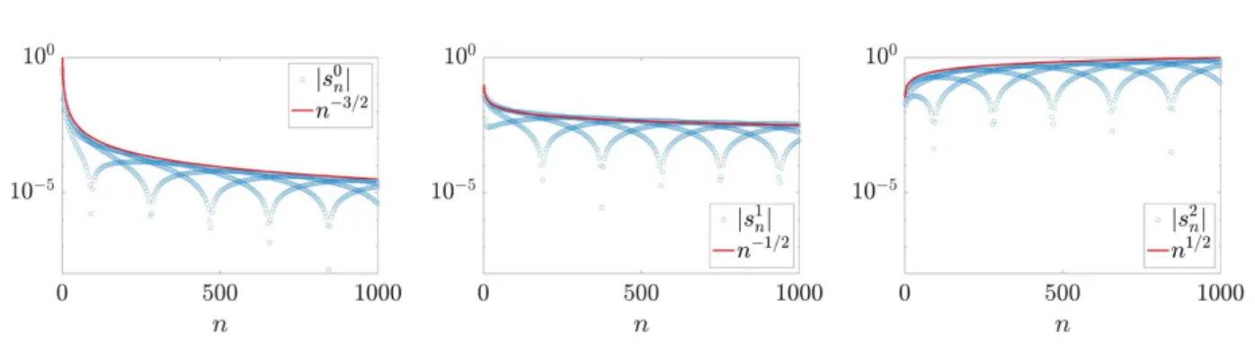
the asymptotic behavior of (𝑠2𝑛)𝑛∈N. However, we verify below on some numerical experiments that (𝑠2𝑛)𝑛∈N does not seem to be bounded. It actually seems to grow like√𝑛, see Figure 7, up to an oscillating behavior similar to the one we have exhibited in (3.20) and (4.11). This growth in√𝑛 is consistent with the singularities of the form (𝑧/𝑧0− 1)−3/2 displayed by 𝜅2𝑠. The rigorous justification of this asymptotic behavior is left to a future work.
Figure 7. Asymptotic behaviour of 𝑠0𝑛, 𝑠1𝑛 and 𝑠2𝑛.
Inductive determination of the expansions. As we have already seen in the analysis of the one-dimensional case, the Laurent series of 𝜅0
𝑠can be also determined inductively by plugging the expansion 𝜅0𝑠(𝑧) = ∞ ∑︁ 𝑛=1 𝜎0𝑛 𝑧𝑛, by then first identifying 𝜎0
1 and then deriving a recurrence formula which gives the expression of 𝜎𝑛0 in terms of 𝜎0
1, . . . , 𝜎𝑛−10 . This led to the formula (3.21). This strategy can be extended to the “correctors” 𝜅1𝑠 and 𝜅2𝑠. Namely, the function 𝜅1𝑠 is given by the relation (4.7). Since 𝑧 𝜅0𝑠(𝑧) has a finite limit at infinity, we already see on (4.7) that 𝜅1𝑠 tends to zero at infinity. It actually decays like 𝑧−2. Hence its Laurent series expansion reads
𝜅1𝑠(𝑧) = ∞ ∑︁ 𝑛=1 𝜎1 𝑛 𝑧𝑛,
and the coefficients (𝜎1𝑛)𝑛≥1 are computed by plugging the latter expression in (4.7) (which itself has been obtained by differentiating (4.2) with respect to 𝜃). After a few simplifications, we obtain 𝜎1
1 = 0 and the recurrence relation ∀ 𝑛 ≥ 1, 𝜎1𝑛+1− 𝜎1 𝑛−1+ 2 𝜇𝑥 𝑛 ∑︁ 𝑚=0 𝜎1𝑚𝜎𝑛−𝑚0 = −𝜇𝑦𝜎𝑛0, where we use the convention 𝜎1
0 = 0. We easily deduce that all odd coefficients 𝜎12 𝑝+1 vanish (recall that the even coefficients 𝜎0
2 𝑚vanish), and the even coefficients 𝜎12 𝑝, which we also write 𝑠1𝑝 to be consistent with (4.9), satisfy 𝑠1 0= 0 and ∀ 𝑛 ≥ 0, 𝑠1𝑛+1 = 𝑠1𝑛− 2 𝜇𝑥 𝑛 ∑︁ 𝑚=0 𝑠1𝑚𝑠0𝑛−𝑚− 𝜇𝑦𝑠0𝑛. (4.16) Recalling the initial values 𝑠0
0= 𝜇𝑥and 𝑠01= 𝜇𝑥(1 − 𝜇2𝑥), we recover for instance from (4.16) the two first values 𝑠1
1= −𝜇𝑥𝜇𝑦 and 𝑠12= −𝜇𝑥𝜇𝑦(2 − 3 𝜇2𝑥) as in the previous method. We can follow the same lines to derive the Laurent series expansion of 𝜅2
𝑠, by starting from the relation (4.12) and plugging (observing on (4.12) that 𝜅2
𝑠 tends to zero at infinity): 𝜅2𝑠(𝑧) = ∞ ∑︁ 𝑛=1 𝜎2 𝑛 𝑧𝑛, which yields 𝜎2
1 = 0 and the recurrence relation ∀ 𝑛 ≥ 1, 𝜎𝑛+12 − 𝜎2 𝑛−1+ 2 𝜇𝑥 𝑛 ∑︁ 𝑚=0 𝜎𝑚2 𝜎0𝑛−𝑚 = −4 𝜇𝑦𝜎1𝑛− 4 𝜇𝑥 𝑛 ∑︁ 𝑚=0 𝜎𝑚1 𝜎1𝑛−𝑚.