Can We Use Cap Rates To Better Allocate Investments in Commercial Real Estate in a Dynamic Portfolio?
by
Stylianos Avramidis
Diploma in Civil Engineering, 2003 Aristotle University of Thessaloniki, Greece
Submitted to the Program in Real Estate Development in Conjunction with the Center for Real Estate in Partial Fulfillment of the Requirements for the Degree of
Master of Science in Real Estate Development
at the
Massachusetts Institute of Technology
September, 2010
© 2010 Stylianos Avramidis All rights reserved
The author hereby grants to MIT permission to reproduce and to distribute publicly paper and electronic copies of this thesis document
in whole or in part in any medium now known or hereafter created.
Signature of Author____________________________________________________________ Center for Real Estate
July 23, 2010
Certified by___________________________________________________________________ Walter N. Torous
Visiting Professor, Center for Real Estate Thesis Supervisor
Accepted by___________________________________________________________________ David M. Geltner
Chairman, Interdepartmental Degree Program in Real Estate Development
Can We Use Cap Rates To Better Allocate Investments in Commercial Real Estate in a Dynamic Portfolio?
by
Stylianos Avramidis
Submitted to the Program in Real Estate Development in Conjunction with the Center for Real Estate on July 23, 2010 in Partial Fulfillment of the Requirements for the Degree of
Master of Science in Real Estate Development
ABSTRACT
This thesis has a two-fold objective, namely to explore the role of cap rates in predicting the returns to commercial real estate, and to identify how cap rates can be used to improve the allocation of real estate in a dynamic investment portfolio.
Seeking an answer to the first question, we run predictive regressions using data for real estate “All Properties” and for all four major property types, examining the predictability power of cap rates for a forecasting horizon from one to four quarters in the future. Moreover, we examine whether or not stock dividend-price ratio can predict real estate returns, and examine the predictability of stock returns by cap rates and dividend-price ratio.
The analysis confirms that both cap rates and the dividend-price ratio can predict real estate “All Properties” returns for up to one year in the future. Concerning the analysis per property type, the results vary from property type to property type, and for different forecast horizons. Moreover, the analysis shows that stock returns can be predicted by the dividend-price ratio at all forecast horizons, whereas the cap rates seem to have somewhat limited predictive power regarding the stock returns. We approach the second question by following the dynamic portfolio allocation methodology proposed by Brandt and Santa-Clara (2006). We expand the existing set of “basis” assets comprised of stocks and real estate to include “conditional” portfolios, and then compute the portfolio weights of this expanded set of assets by applying the Markowitz solution to the optimization problem. We apply this methodology to three different portfolio rebalancing horizons. Moreover, we work with three cases for each portfolio, i.e. with the unconditional case, with the case where the dividend-price ratio is the only conditioning variable, and with the case where the cap rate is the second conditioning variable. In almost all instances the results confirm that, by adding the cap rate as an additional state variable, the performance of the portfolios increases significantly. The same conclusion stands when we impose a “no shorting” restriction to real estate, although now the role of cap rates seems somewhat less significant.
Table of Contents
Abstract ... 2
Table of Contents ... 3
Table of Exhibits ... 4
Acknowledgements ... 5
1. Introduction and Background ... 6
1.1. Introduction ... 6
1.2. Addition to Current Body of Knowledge ... 7
2. Research Data ... 8
2.1. Data Description ... 8
2.2. Commercial Real Estate Data ... 8
2.3 Data on Stocks ... 10
3. Prediction of Future Returns in Commercial Real Estate and Stocks ... 11
3.1. Predictive Regression Methodology ... 11
3.2. Prediction of Expected Returns to Commercial Real Estate and Stocks using Historical Data on Cap Rates and the Dividend-Price Ratio ... 12
3.3. Predictive Regression Results ... 14
4. Dynamic Allocation of Commercial Real Estate in a Risky Asset Portfolio ... 19
4.1. Dynamic Portfolio Allocation Methodology ... 19
4.2. Application of the Dynamic Asset Allocation Methodology ... 23
4.3. Results of the Dynamic Portfolio Analysis with Quarterly Rebalancing ... 28
4.4. Results of the Dynamic Portfolio Analysis with Semi-Annual Rebalancing ... 42
4.5. Results of the Dynamic Portfolio Analysis with Annual Rebalancing ... 53
5. Summary and Conclusions ... 64
5.1. The Use of Cap Rates and Dividend-Price Ratio to Predict Future Returns to Commercial Real Estate and Stocks ... 64
5.2. The Use of Cap Rates in Allocating Investments in Commercial Real Estate in a Dynamic Portfolio ... 65
5.3. Study Limitations and Scope for Further Research ... 65
Table of Exhibits
Prediction of Expected Returns to Commercial Real Estate and Stocks (Section 3.3.)
Exhibit 1: Predictive Regression Summary Output ... 14
Dynamic Portfolio Optimization with Quarterly Rebalancing Portfolios (Section 4.3.) Exhibit 2: Stocks and R.E. “All Properties” Portfolio Analysis ... 28
Exhibit 3: Stocks and R.E. Apartment Portfolio Analysis ... 30
Exhibit 4: Stocks and R.E. Industrial Portfolio Analysis ... 32
Exhibit 5: Stocks and R.E. Office Portfolio Analysis ... 34
Exhibit 6: Stocks and R.E. Retail Portfolio Analysis ... 36
Dynamic Portfolio Optimization with Semi-Annual Rebalancing Portfolios (Section 4.4.) Exhibit 7: Stocks and R.E. “All Properties” Portfolio Analysis ... 42
Exhibit 8: Stocks and R.E. Apartment Portfolio Analysis ... 44
Exhibit 9: Stocks and R.E. Industrial Portfolio Analysis ... 46
Exhibit 10: Stocks and R.E. Office Portfolio Analysis ... 48
Exhibit 11: Stocks and R.E. Retail Portfolio Analysis ... 50
Dynamic Portfolio Optimization with Annual Rebalancing Portfolios (Section 4.5.) Exhibit 12: Stocks and R.E. “All Properties” Portfolio Analysis ... 53
Exhibit 13: Stocks and R.E. Apartment Portfolio Analysis ... 55
Exhibit 14: Stocks and R.E. Industrial Portfolio Analysis ... 57
Exhibit 15: Stocks and R.E. Office Portfolio Analysis ... 59
Acknowledgements
As the author of the current work, I am extremely grateful to my thesis advisor, Professor Walter N. Torous, for the advice and guidance he provided me with throughout the process of preparing this paper. His wisdom and inputs on various aspects of the thesis were truly inspirational, whereas his patience, understanding and encouragement supported my effort in every step of this intellectual challenge.
Moreover, I would like to express my sincere thanks to all faculty and staff of MIT Center for Real Estate for giving me the opportunity to work with them, and for the valuable experience and knowledge I gained during the year of my pursuing the Master’s degree in Real Estate Development.
Last, but definitely not least, I would like to thank my family, without the support of whom I wouldn’t be at MIT.
1. Introduction and Background
1.1. Introduction
This thesis has a two-fold objective, namely to explore the role of cap rates in predicting the returns to commercial real estate, and to identify how cap rates can be used to improve the allocation of real estate in a dynamic investment portfolio.
The first question of how, and to what degree, do cap rates predict the returns to commercial real estate, is a question of major importance for investors. A similar question of how the dividend‐price ratio can predict returns in the stock market has been extensively explored, and the results are supportive of the opinion that this kind of relation should be examined in the world of commercial real estate, too.
In order to deal with that issue we follow a simplified version of the predictive regressions methodology implemented by Plazzi, Torous and Valkanov (2010), and run a series of predictive regressions to examine the predictability power of cap rates for periods ranging from one to four quarters in the future. This forecasting horizon was chosen because it covers the most commonly used timeframe in portfolio analysis and portfolio rebalancing, which is explored in the second part of this thesis.
Additionally, since the results from this part of the thesis will be used to confirm our findings in the second part, it was considered necessary to expand our analysis in identifying whether or not the stock market’s dividend-price ratio can predict real estate returns. Moreover, and for the same reason as above, we further explore the predictability of stock returns by the cap rates and dividend-price ratio.
The second question which will be examined in this thesis is how investors can use the results from the aforementioned analysis so as to better allocate commercial real estate in a dynamic, risky asset portfolio, so as to achieve better portfolio performance.
portfolios. This fact has major implications for portfolio managers, since it influences the strategic decision making of how to allocate the wealth of these large institutional “players” among the various investment classes, so as to gain the maximum possible returns while being exposed to the minimum possible risk. Moreover, nowadays there are new approaches proposed by the academic world that can help portfolio managers apply a dynamic portfolio selection, which is considered a much better approach to portfolio analysis, without facing the severe computational difficulties of past methodologies.
One of the novel methodologies proposed is that of Brandt and Santa-Clara (2006), and is the one we will follow in the second part of the current thesis. This approach, although quite data intensive for long horizons, is very intuitive and simple to apply. It is based on the rationale that we can expand an existing set of “basis” assets so as to include mechanically managed, “conditional” portfolios, and then compute the static portfolio weights of this expanded set of assets by applying the traditional Markowitz solution to the optimization problem.
The organization of this thesis is as follows: Chapter 1 includes a brief introduction to the concepts the current thesis will be dealing with. Chapter 2 describes the real estate and stock databases and discusses the data used. Chapter 3 describes the predictive regression methodology followed and includes the analysis results from the series of predictive regressions we have run. Chapter 4 outlines the dynamic portfolio methodology of Brandt and Santa-Clara (2006) and includes the results of its application to the data of this thesis. Chapter 5 concludes and expresses some thoughts on topics that might be of interest for future research. Chapter 6 shows the references used.
1.2. Addition to Current Body of Knowledge
Of course, there has been significant work done on this important topic by, among others, Plazzi, Torous and Valkanov, (2010); this thesis is intended to add to the current body of knowledge by using techniques, database recourses, and a historical examination period which differ from those utilized in previous papers. For a more detailed description of the data and methodology employed in each case, please refer to the corresponding chapters.
2. Research Data
2.1. Data Description
The data requirements for this thesis reflect the quantitative nature of the topic, and require access to both real estate and stock databases. More specifically, in the case of real estate we are using the historical data on cap rates from the NPI index, and data on returns from the TBI index. The data collected concern the main “All Properties” index and the four major real estate property types (Apartment, Industrial, Office, and Retail buildings) for the 1984Q2-2010Q1 and 1994Q2-2010Q1 periods, respectively.
As far as the data for stocks is concerned, we use the historical S&P500 total returns and the corresponding dividend-price ratios, which are made publicly available by Standard & Poor’s for the aforementioned historical periods. Moreover, we use the US Treasury T-Bills with a 3-month maturity period as an approximation of the risk-free rate; data on the T-Bills were collected from the Federal Reserve Bank website.1
Furthermore, please note that the “raw” data, as provided by the sources above, are reported in monthly and quarterly time intervals, which differ from those we utilize in our analysis. Therefore, the data were adjusted accordingly to match the time intervals used in this thesis (our analysis is on a quarterly, semi-annual and annual basis).
For definitions and more detailed descriptions on the aforementioned databases and on the specific data used for the purposes of this thesis, the reader can refer to Sections 2.2. and 2.3. to follow.
2.2. Commercial Real Estate Data
At that point we start by briefly introducing the reader to the NCREIF database and, more specifically, to the characteristics of the NPI index, which provides us with some of the data that will be used in the current thesis.
The National Council of Real Estate Investment Fiduciaries (NCREIF) is an institutional real estate investment association which dates its origins to the mid 1970s. NCREIF collects data from its contributing members that concern both individual commercial properties and investment funds, and utilizes these for creating the quarterly NCREIF Property Index (NPI), among other indices.2
As of the first quarter of 2010, there are 6,067 individual properties in the NCREIF database from which the NPI is constructed. Moreover, and in addition to the main NPI “All Properties” index, NCREIF publishes sub-indices for the four main property types (Apartment, Industrial, Office, and Retail buildings).
From this database we will be using the quarterly historical cap rates for each of the real estate categories above, and more specifically the “equal-weighted cap rate four-quarter moving average”. Based on the methodology applied by NPI, the quarterly cap rates are calculated by dividing the actual accounting NOI income from properties that are revalued during each quarter. Then, the “four-quarter moving average cap rate” is set up to be equal to the average of the cap rate of each “four-quarter and the quarterly cap rates from three periods back in the past.
The NPI is the most widely used indicator measuring the performance of institutional quality commercial real estate in the US. However, the NPI is, by definition, an “appraisal-based index with staggered appraisals”, a fact which means that it is based on the cross-sectional aggregate appraisal values at the property level, however without all properties included in the index being reappraised as of the same point in time [Geltner, Miller, Clayton and Eichholtz (2006), pp. 676-677]. As a consequence, the NPI index is based on “stale appraisals”, thus suffering from “lagging” and “smoothing”, which makes the index ineffective in some applications, such as portfolio optimization.3
In order to address the issues that arise from the appraisal-based nature of NCREIF, the MIT Center for Real Estate launched in 2006 a new index, the “Transactions-Based Index (TBI) of Institutional
_____________________________________________________________________________________________
2
For more details on the organization, and on the process it follows to produce the aforementioned index, we recommend that the reader refer to the NCREIF website: www.ncreif.org
3
Fisher, Jeff D., Geltner, David M., and Henry O. Pollakowski, 2007, A Quarterly Transactions-Based Index (TBI) of Institutional Real Estate Investment Performance and Movements in Supply and Demand, Journal of Real Estate Finance and Economics 34, 5-33
Commercial Property Investment Performance”. The TBI is a transactions-based index complementary to the NPI, which uses econometric techniques to estimate the market movements and returns on investment based on transaction prices of properties sold from the NPI database each quarter [Fisher, Geltner, and Pollakowski (2007)].
Since a large part of the current thesis involves portfolio optimization, the TBI database was considered more precise and appropriate than the NPI. Thus, from the former database we will be using the quarterly historical returns for the “All Properties” and for each of the four main property types mentioned above.4 Please note that the TBI returns are comparable to the so-called NPI’s “equal-weighted cash-flow based returns, with appreciation including capital expenditures” [Fisher, Geltner, and Pollakowski (2007)].
2.3. Data on Stocks
In this thesis we will be using the historical S&P500 database for the data on stocks that we need for our analysis. The S&P 500 is one of the most commonly used indices in analyzing the performance of the US-based, large cap common stocks, and it includes data since 1957. It is a capitalization-weighted index that considers the 500 large-cap American stocks, and its database is publicly available by Standard & Poor’s. 5
From this database we will be using the historical total returns of that index for the aforementioned period, namely from 1984Q2 until 2010Q1. The data are reported on a monthly basis, so they were adjusted accordingly in the time intervals we are considering in this paper. Moreover, for the same period, we use the “four-quarter moving average” dividend-price ratio reported by S&P, which has a similar structure to that of the NPI’s “four-quarter moving average” cap rates.
_____________________________________________________________________________________________
4
3. Prediction of Future Returns in Commercial Real Estate and Stocks
3.1. Predictive Regression Methodology
In this chapter we examine the ability that the cap rate and dividend-price ratio have in predicting real estate and stock returns, following a simplified version of the predictive regressions methodology implemented by Plazzi, Torous and Valkanov (2010). More specifically, we will be focusing on the relation between the asset returns and the lagged predictive variables, however without creating a system of “structural” equations, which is normally required to apply additional restrictions so as to express the dynamics among the various predictive variables used in each case.6
The form of the predictive regression model we will be using involves a linear relation between the value of an asset and a lagged variable, which variable’s value should already be known at the beginning of each period, so as to play the role of a predictor. The form of this OLS regression model is given by the expression [Stambaugh (1999), p.376]:
1 1 t t t y+ =α+βx +ε+ (1) where: 1 t
y+ reflects a change in the asset’s value during the period from time t to t+1 t
x is the lagged regressor-variable, related to the asset’s value, and known at time t
,
a
β
are coefficients to be estimated 1t
ε+ are the regression “residuals”
The equation above, although it refers to a single time period, it can be set up in an even more general way, which will enable us to examine the predictability power of the lagged variables at longer time horizons. That being the case, we will use the following regression formula to predict an asset’s value over a longer horizon of k>1 periods [Plazzi, Torous and Valkanov (2010), p.7]:
_____________________________________________________________________________________________
6
The Plazzi, Torous and Valkanov (2010) paper includes a detailed methodology on how to construct a system of “structural” equations for predictive purposes, and is focused on the case of real estate. For an application of a similar methodology to the case of stocks, the reader may refer to:
Campbell, John Y., and Robert J. Shiller, 1988b, The Dividend-Price Ratio and Expectation of Future Dividends and Discount Factors, Review of Financial Studies 1, 195-228.
1 1 t t k k k t t t k y+ → + =α +β x +ε+ → + (2) where: 1 1 0 k t t k t i i y+ → + y+ + = =
∑
(3)3.2. Prediction of Expected Returns to Commercial Real Estate and Stocks using Historical Data on Cap Rates and the Dividend-Price Ratio
By using the predictive regression models given by equations (1) and (2), we will now test whether or not, and to what degree, cap rates and the dividend-price ratio can predict the returns to commercial real estate and stocks. Our focus will be to examine the predictability of the returns to these two asset classes using quarterly time intervals within a one year timeframe, which is the most commonly used timeframe in portfolio analysis and portfolio rebalancing.
At this point it is also worth mentioning that the predictive regressions expressed by formula (2), combined with equation (3), require using overlapping data for returns in the left-hand side of equation (2). In order to deal with this issue, we apply the methodology proposed by Newey-West (1987b)7, setting the Newey-West estimator q in each regression equal to the number of lags that correspond to the number of periods we want to predict the returns for, going forward in the future.
So, in the case of real estate, we will be applying the following regression formulas:
(
)
(
)
1 1 1 1 1 1 RE t t t RE t t k k k t t t k r cap r capα
β
ε
α
β
ε
+ + + → + + → + = + + = + + (4) and(
)
(
)
1 1 1 1 1 1 RE t t t RE t t k k k t t t k r dy r dyα
β
ε
α
β
ε
+ + + → + + → + = + + = + + (5) _____________________________________________________________________________________________ 7As far as the case of stocks is concerned, the forecasting regressions take the form:
(
)
(
)
1 1 1 1 1 1 S t t t S t t k k k t t t k r dy r dyα
β
ε
α
β
ε
+ + + → + + → + = + + = + + (6) and(
)
(
)
1 1 1 1 1 1 S t t t S t t k k k t t t k r cap r capα
β
ε
α
β
ε
+ + + → + + → + = + + = + + . (7)In this section we will be using historical quarterly data for the returns, cap rates and the dividend-price ratio to study the predictability of returns for k=1, 2, 3 and 4 quarters going forward at each point in the sample period. Accordingly, we will be regressing the log excess returns (gross returns minus the risk-free rate) of each asset with each of the prediction variables, also expressed in logarithm form. The results of the forecasting regressions are shown in Exhibit 1 to follow.
3.3. Predictive Regression Results
Exhibit 1: Predictive Regression Summary Output
Table 1.1: Commercial Real Estate Excess Returns regressed against corresponding Cap Rates
k Coeff. α Std. Error α t Stat α Coeff. β Std. Error β t Stat β R^2 Adj. R^2 S.E. of Regr. F Stat 1 -0.073343 0.029424 -2.492604 4.216335 1.550554 2.719244 0.068217 0.058991 0.042962 7.394289 2 -0.154187 0.084598 -1.822593 8.860487 4.115906 2.152743 0.136867 0.128236 0.061466 15.857062 3 -0.240755 0.128668 -1.871131 13.816903 6.214027 2.223502 0.191049 0.182878 0.078547 23.380766 4 -0.343539 0.167673 -2.048871 19.567742 8.031953 2.436237 0.252913 0.245290 0.092562 33.176188
k Coeff. α Std. Error α t Stat α Coeff. β Std. Error β t Stat β R^2 Adj. R^2 S.E. of Regr. F Stat 1 -0.031590 0.027541 -1.147015 2.717027 1.573870 1.726335 0.046581 0.030951 0.043399 2.980232 2 -0.067767 0.090985 -0.744809 5.655661 4.642791 1.218160 0.083835 0.068566 0.066248 5.490390 3 -0.098103 0.138535 -0.708142 8.299472 7.045621 1.177962 0.099264 0.083997 0.088783 6.501984 4 -0.138343 0.184372 -0.750348 11.593448 9.323532 1.243461 0.124255 0.109156 0.109141 8.229303
k Coeff. α Std. Error α t Stat α Coeff. β Std. Error β t Stat β R^2 Adj. R^2 S.E. of Regr. F Stat 1 -0.077065 0.045291 -1.701555 4.522622 2.257248 2.003600 0.061747 0.046365 0.055014 4.014413 2 -0.160956 0.136531 -1.178899 9.442792 6.244187 1.512253 0.126978 0.112428 0.077502 8.726815 3 -0.250420 0.214819 -1.165727 14.638700 9.773935 1.497728 0.186417 0.172628 0.095773 13.518735 4 -0.349182 0.285446 -1.223285 20.261914 12.931948 1.566811 0.224084 0.210706 0.117471 16.750368
k Coeff. α Std. Error α t Stat α Coeff. β Std. Error β t Stat β R^2 Adj. R^2 S.E. of Regr. F Stat 1 -0.062702 0.032178 -1.948597 3.937124 1.633635 2.410039 0.086940 0.071971 0.042726 5.808289 2 -0.140087 0.124349 -1.126569 8.568009 5.797620 1.477849 0.149817 0.135647 0.068685 10.573047 3 -0.226884 0.186085 -1.219248 13.799716 8.628788 1.599265 0.191623 0.177922 0.095496 13.985779 4 -0.316520 0.241569 -1.310271 19.166161 11.146828 1.719427 0.229043 0.215751 0.117845 17.231190
k Coeff. α Std. Error α t Stat α Coeff. β Std. Error β t Stat β R^2 Adj. R^2 S.E. of Regr. F Stat 1 -0.039722 0.037399 -1.062095 2.722393 1.874764 1.452126 0.033413 0.017568 0.044762 2.108671 2 -0.092331 0.092947 -0.993366 6.076085 4.330518 1.403085 0.068128 0.052597 0.068866 4.386545 3 -0.152183 0.142045 -1.071368 9.833005 6.596278 1.490690 0.099409 0.084145 0.090766 6.512565 4 -0.216236 0.188786 -1.145405 13.838795 8.750302 1.581522 0.124986 0.109900 0.111894 8.284662
Real Estate Apartment Returns against Apartment Cap Rates
Real Estate Industrial Returns against Industrial Cap Rates
Real Estate Office Returns against Office Cap Rates
Real Estate Retail Returns against Retail Cap Rates
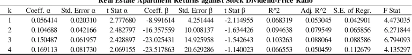
Table 1.2: Commercial Real Estate Excess Returns regressed against the Stock Dividend-Price Ratio
Table 1.3: Stock Excess Returns regressed against the Dividend-Price Ratio
k Coeff. α Std. Error α t Stat α Coeff. β Std. Error β t Stat β R^2 Adj. R^2 S.E. of Regr. F Stat 1 0.038301 0.012213 3.136159 -5.352705 1.889520 -2.832839 0.073607 0.064435 0.042838 8.024975 2 0.073492 0.025572 2.873977 -10.056804 3.825154 -2.629124 0.118505 0.109690 0.062116 13.443607 3 0.102557 0.040843 2.510975 -13.681025 5.739261 -2.383761 0.127089 0.118272 0.081593 14.413604 4 0.133131 0.056342 2.362909 -17.715683 7.610046 -2.327934 0.142957 0.134212 0.099140 16.346698
k Coeff. α Std. Error α t Stat α Coeff. β Std. Error β t Stat β R^2 Adj. R^2 S.E. of Regr. F Stat 1 0.056414 0.020310 2.777680 -8.991614 4.251444 -2.114955 0.068319 0.053045 0.042901 4.473035 2 0.104688 0.042166 2.482797 -16.357559 10.008137 -1.634426 0.094638 0.079549 0.065856 6.271844 3 0.150487 0.061957 2.428897 -23.025431 14.925958 -1.542643 0.103263 0.088064 0.088586 6.794093 4 0.169113 0.081730 2.069155 -23.517863 20.629286 -1.140023 0.066553 0.050459 0.112679 4.135297
k Coeff. α Std. Error α t Stat α Coeff. β Std. Error β t Stat β R^2 Adj. R^2 S.E. of Regr. F Stat 1 0.065666 0.025947 2.530777 -11.521615 5.431524 -2.121249 0.068698 0.053431 0.054809 4.499698 2 0.111188 0.046496 2.391334 -18.384387 11.511819 -1.597001 0.083233 0.067954 0.079420 5.447413 3 0.144309 0.062330 2.315260 -22.519304 16.138478 -1.395380 0.076668 0.061019 0.102029 4.899030 4 0.175028 0.082311 2.126437 -26.271439 21.779142 -1.206266 0.063517 0.047370 0.129055 3.933834
k Coeff. α Std. Error α t Stat α Coeff. β Std. Error β t Stat β R^2 Adj. R^2 S.E. of Regr. F Stat 1 0.061076 0.020213 3.021642 -10.276307 4.231204 -2.428696 0.088172 0.073224 0.042697 5.898562 2 0.117494 0.063304 1.856035 -19.768289 14.564321 -1.357309 0.119324 0.104646 0.069906 8.129515 3 0.151616 0.094276 1.608214 -23.867290 22.246494 -1.072856 0.086068 0.070577 0.101540 5.556202 4 0.162139 0.118412 1.369271 -22.781599 28.792842 -0.791224 0.047157 0.030729 0.131010 2.870490
k Coeff. α Std. Error α t Stat α Coeff. β Std. Error β t Stat β R^2 Adj. R^2 S.E. of Regr. F Stat 1 0.060658 0.020642 2.938591 -10.139883 4.321019 -2.346642 0.082800 0.067763 0.043603 5.506728 2 0.134338 0.053889 2.492874 -23.181406 10.372238 -2.234947 0.178907 0.165222 0.064643 13.073319 3 0.197964 0.079145 2.501278 -33.912509 14.886267 -2.278107 0.214287 0.200970 0.084779 16.091051 4 0.252170 0.102639 2.456874 -42.587954 19.322254 -2.204088 0.207465 0.193801 0.106490 15.182916
Real Estate Apartment Returns against Stock Dividend-Price Ratio
Real Estate Industrial Returns against Stock Dividend-Price Ratio
Real Estate Office Returns against Stock Dividend-Price Ratio
Real Estate Retail Returns against Stock Dividend-Price Ratio Real Estate "All Properties" Returns against Stock Dividend-Price Ratio
k Coeff. α Std. Error α t Stat α Coeff. β Std. Error β t Stat β R^2 Adj. R^2 S.E. of Regr. F Stat 1 -0.028930 0.023636 -1.223984 7.252082 3.656930 1.983106 0.037478 0.027948 0.082907 3.932711 2 -0.061311 0.046998 -1.304557 14.896803 5.894222 2.527357 0.073559 0.064294 0.119725 7.939931 3 -0.093673 0.071812 -1.304419 22.492736 8.748794 2.570953 0.108302 0.099295 0.146871 12.024098 4 -0.120939 0.095543 -1.265812 29.000101 11.427090 2.537838 0.134539 0.125708 0.168109 15.234455
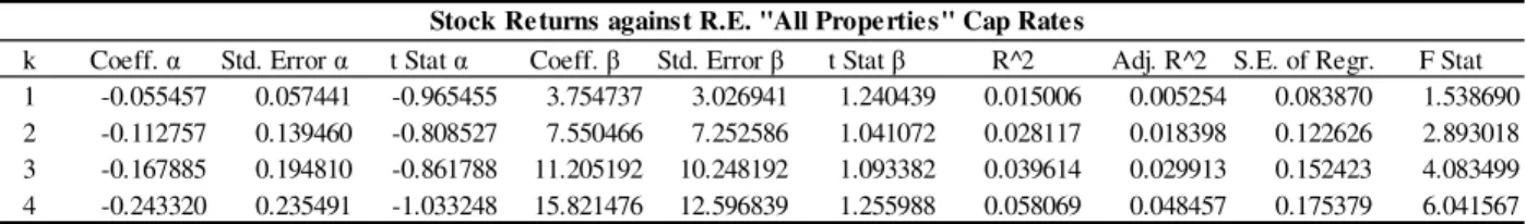
Table 1.4: Stock Excess Returns regressed against Commercial Real Estate Cap Rates
k Coeff. α Std. Error α t Stat α Coeff. β Std. Error β t Stat β R^2 Adj. R^2 S.E. of Regr. F Stat 1 -0.055457 0.057441 -0.965455 3.754737 3.026941 1.240439 0.015006 0.005254 0.083870 1.538690 2 -0.112757 0.139460 -0.808527 7.550466 7.252586 1.041072 0.028117 0.018398 0.122626 2.893018 3 -0.167885 0.194810 -0.861788 11.205192 10.248192 1.093382 0.039614 0.029913 0.152423 4.083499 4 -0.243320 0.235491 -1.033248 15.821476 12.596839 1.255988 0.058069 0.048457 0.175379 6.041567
k Coeff. α Std. Error α t Stat α Coeff. β Std. Error β t Stat β R^2 Adj. R^2 S.E. of Regr. F Stat 1 -0.056919 0.055463 -1.026256 3.991180 3.169465 1.259260 0.025337 0.009359 0.087397 1.585736 2 -0.112562 0.128363 -0.876904 7.825852 7.072960 1.106447 0.041714 0.025742 0.132909 2.611783 3 -0.175321 0.181300 -0.967022 12.024128 10.174006 1.181848 0.058060 0.042095 0.171990 3.636707 4 -0.251686 0.222712 -1.130096 16.771231 12.796994 1.310560 0.079240 0.063365 0.202726 4.991430
k Coeff. α Std. Error α t Stat α Coeff. β Std. Error β t Stat β R^2 Adj. R^2 S.E. of Regr. F Stat 1 -0.092273 0.071628 -1.288228 5.235265 3.569878 1.466511 0.034056 0.018221 0.087005 2.150655 2 -0.185500 0.173679 -1.068060 10.443422 8.436366 1.237905 0.057970 0.042269 0.131776 3.692236 3 -0.283808 0.240795 -1.178631 15.856373 11.818173 1.341694 0.078522 0.062904 0.170111 5.027598 4 -0.410806 0.282799 -1.452646 22.487847 14.129493 1.591554 0.109983 0.094638 0.199313 7.167267
k Coeff. α Std. Error α t Stat α Coeff. β Std. Error β t Stat β R^2 Adj. R^2 S.E. of Regr. F Stat 1 -0.094923 0.065222 -1.455381 5.481838 3.311224 1.655532 0.042999 0.027310 0.086601 2.740786 2 -0.194252 0.162665 -1.194186 11.115536 8.034730 1.383436 0.075903 0.060501 0.130516 4.928253 3 -0.299425 0.220699 -1.356714 16.992507 10.959485 1.550484 0.104376 0.089196 0.167708 6.875846 4 -0.435894 0.249608 -1.746315 24.237208 12.560427 1.929648 0.147819 0.133126 0.195030 10.060655
k Coeff. α Std. Error α t Stat α Coeff. β Std. Error β t Stat β R^2 Adj. R^2 S.E. of Regr. F Stat 1 -0.058617 0.073404 -0.798548 3.557159 3.679638 0.966714 0.015089 -0.001057 0.087855 0.934536 2 -0.120209 0.190945 -0.629548 7.195606 9.492769 0.758009 0.026379 0.010152 0.133968 1.625610 3 -0.190712 0.268642 -0.709910 11.243125 13.512334 0.832064 0.037858 0.021551 0.173824 2.321541 4 -0.283006 0.326456 -0.866905 16.183756 16.744495 0.966512 0.054796 0.038500 0.205399 3.362429
Stock Returns against R.E. "All Properties" Cap Rates
Stock Returns against R.E. Apartment Cap Rates
Stock Returns against R.E. Industrial Cap Rates
Stock Returns against R.E. Office Cap Rates
In order to make it easier to follow the author’s comments on the findings of the regression analysis above, the results will be presented separately for each table.
Comments on Table 1.1
As we can see in Table 1.1, where the results of the Commercial Real Estate returns regressed against cap rates are shown, the “All Properties” returns can be predicted by the corresponding cap rates at all time horizons (k=1 to 4), showing statistically significant t-stats (larger than 2) for the cap rate coefficient β. Moreover, we can see that the longer the forecasting horizon, the larger the R2 gets, which starts with a value of 6.8% for k=1, reaching 25.2% for k=4.
As far as the Industrial and Office returns are concerned, we see that at the short horizon of a quarter (k=1), cap rates can predict returns, explaining 6.17% and 8.69% of the variability in returns, respectively. Furthermore, for the longer forecasting horizons we see that the predictability power decreases (lower t-stats), however it remains somewhat significant (t-stats around 1.5 to 1.7), with the R2 increasing throughout, being for both cases more than 22%, for k=4.
Finally, for the cases of Apartment and Retail, we see that the cap rates can somewhat predict returns, since we have the t-stat of the β coefficient moving within a wide range of values, i.e. between 1.1 and 1.7. In this case we observe an increase in the R2 as the forecasting horizon increases, but with lower R2 values compared to the previous case of Industrial and Office buildings.
Comments on Table 1.2
Checking the results from Table 1.2, where Real Estate returns are regressed against the Stock dividend-price ratio, we can see that the “All Properties” and Retail returns can be predicted by the dp ratio at all forecasting horizons (k=1 to 4), having statistically significant t-stat values for the dp ratio β coefficient. Furthermore, for the longer forecasting horizons we see that the R2 is increasing, and even reaching 20% in the case of Retail with k=4.
For the case of Apartment, Industrial and Office buildings, we see they follow a prediction “pattern”, where the dividend-price ratio can predict the returns in the short-run (k=1), and as the forecasting
horizon increases, the t-stats are getting less significant. Please note that the R2 in all of these cases appears to be much less volatile compared to the case of “All Properties” and Retail discussed above.
Comments on Table 1.3
Moving to stocks, we can see from Table 1.3 that the dividend-price ratio can predict stock returns at all forecasting horizons (k=1 to 4), having statistically significant t-stat values for the dp ratio β coefficient. As far as the R2 is concerned, its value increases significantly as the forecasting horizon increases, starting with a value of just 3.74% for k=1, and reaching up almost 13.5% for k=4.
Comments on Table 1.4
Turning our attention to the ability of the cap rates to predict stock returns, we can see in Table 1.4 that the results are less significant, compared to the cases of the previous tables. More specifically, the t-stats show a limited ability of the cap rates to predict stock returns for all cases, since the t-stats that correspond to the cap rates range almost exclusively between 1.0 and 1.5.
We can see two exceptions to the aforementioned “pattern”. One has to do with the fact that the t-stats in Retail properties have all insignificant values, less than 1.0. The other exception is the t-stat value we got for Office in the case of k=4, where we have a significant t-stat value almost equal to 2, explaining about 15% of the variability in returns.
4. Dynamic Allocation of Commercial Real Estate in a Risky Asset Portfolio
4.1. Dynamic Portfolio Allocation Methodology
We now introduce the reader to the dynamic portfolio allocation methodology followed in this chapter, and more specifically, to the Brandt and Santa-Clara (2006) approach outlined in their paper the “Dynamic Portfolio Selection by Augmenting the Asset Space” (reference [1]).
The intuition behind this methodology is to expand the existing set of “basis” assets used in the dynamic portfolio analysis so as to include mechanically managed, “conditional” portfolios, and then compute the static portfolio weights of this expanded set of assets by applying the traditional Markowitz solution to the optimization problem. Hence, the time-varying weights invested in each “basis” asset in the dynamic portfolio are expressed as a linear function of the parameterized weights of the “basis” asset and its corresponding “conditional” assets in the aforementioned static portfolio.
To make things easier, we start by defining a few concepts which will be used throughout this chapter. Firstly, “conditional” portfolios are defined as mechanically constructed portfolios that invest in each “basis” asset (for instance stocks) an amount proportional to the level of the conditioning variable in each time period. Secondly, the conditioning variables are those factors, for which there is evidence that they can predict the returns of the “basis” assets (such is the case of dividend-price ratio, which can predict the stock market returns, as we saw in the previous chapter).
Moreover, please note that throughout this chapter we will be working with asset excess returns, which are calculated by the equation:
1 1 i i f t t t r+ =R+ −R (8) where: 1 i t
r+ is the excess return of the “basis” asset i at time t+1
1 i t
R+ is the total (gross) return of asset i at time t+1 f
t
The rationale for using excess returns is that by doing so, we implicitly presume that the remainder of the portfolio’s value is invested in the risk-free asset (3-month US T-Bills), with a return equal to R tf
[Brandt and Santa-Clara (2006), p.2191].
Now, assuming that we have N “basis”, risky assets and K “conditional”, state variables, we define the time-varying vectors of excess returns rt+1
(
N×1)
and state variables z t(
K×1)
as in (9) below. Please note that the first value of the state variables is taken to be a constant equal to 1, which reflects the static mean-variance case (no conditioning variables applied).1 1 2 1 1 1 t t t N t r r r r + + + + = L , 1 1 1 t t K t z z z − = L (9) where: 1 i t
r+ is the excess return of the “basis” asset i at time t+1 (i=1, 2…N denotes a different “basis” asset) j
t
z is the value of the conditioning variable j at time t (j=1, 2…K-1 denotes a different state variable).
Furthermore, we construct a
(
N×1)
vector of the parameterized, time-varying portfolio weightsx , tand a
(
N K×)
coefficient matrixθ
. These matrices are related to each other in such a way so as to satisfy equation (10) given below, thus defining a system of linear equalities, and relating the state variables vector z to the portfolio weights vector t x (ibid, p.2190): t1 1 1 1 11 12 1 11 12 1 1 2 2 1 1 21 22 2 21 22 2 1 1 1 1 2 1 2 1 K t t t t K t t t t t t t K N N K t t t N N t N t x x z z z x x z z x z z x x z z θ θ θ θ θ θ θ θ θ θ θ θ θ θ θ θ θ θ θ − Κ Κ − Κ Κ − − Ν Ν ΝΚ Κ = + + + = + + + = ⇒ = × ⇒ = + + + L L L L L L L L L L L L L (10) where: i t
x is the weight of the “basis” asset i at time t (i=1, 2…N denotes a different “basis” asset)
Next we define the expanded static portfolio, which is equivalent to the dynamic portfolio with N “basis” assets. This static portfolio is a portfolio which includes (NK) assets, and is comprised of both “basis” and “conditional” assets. For this expanded portfolio, the returns of the “basis” assets at time t+1 are taken from the database used in each case, whereas the returns of the “conditional” assets are created by multiplying the returns of the “basis” assets at time t+1 with the value of the state variables at time t (ibid, p.2198). Therefore, we now have an expanded static portfolio, which has a time series of t+1 observations of the form below (ibid, p.2199):
N “basis” Assets N Assets “conditional” on z1 N Assets “conditional” on zk-1
1 2 1 1 1 2 1 1 1 1 2 1 1 1 1 0 1 0 1 0 1 0 1 0 1 0 1 1 2 1 1 1 2 1 1 1 1 2 1 2 2 2 1 2 1 2 1 2 1 2 1 2 1 2 1 2 1 1 1 2 1 1 1 1 2 1 1 1 1 1 1 1 1 1 1 N N K K K N N N K K K N N N K K K N t t t t t t t t t t t t t t t r r r z r z r z r z r z r z r r r r z r z r z r z r z r z r r r r z r z r z r z r z r z r − − − − − − − − − + + + + + + + + + L L L L L L L L L L L L L L L L L L L L L L L L L (11) where: 1 i t
r+ is the excess return of the “basis” asset i at time t+1 (i=1, 2…N denotes a different “basis” asset) j
t
z is the value of the conditional variable j at time t (j=1, 2… K-1 denotes a different state variable).
Please note that the difference in dating between the returns and the state variables reflects the fact that the state variables should be known at the beginning of each return period, as they play the role of predictors (ibid, p.2198).
Considering now the assumptions of the static portfolio theory [Markowitz (1952)] that the investor’s goal is to maximize the expected returns over a single period going forward in the future, and at the same time minimize the risk, the optimization problem of the dynamic portfolio can be expressed as an optimization problem of the newly created static portfolio. Therefore, the optimization problem can be expressed as [Brandt and Santa-Clara (2006), p.2191]:
1 1 1 max 2 t t t t t t t t x E x r x r r x γ + + + − T T T (12)
where: t
x is the time-varying portfolio weights vector, as defined above (xt =θzt)
1 t
r+ is the excess returns vector of the “basis” assets, as defined above
γ
is a constant reflecting the representative investor’s risk tolerance.In order to solve expression (12) analytically we need to make some additional transformations. For this reason, we define two additional vectors, namely the
(
NK×1)
vectors x% and r%t+1 as follows:[
1 2 NK]
( )
[
11 N1 12 N2 1K NK]
x%= x% x% L x% T =vec θ = θ L θ θ L θ L θ L θ T (13) 1 1 1 1 1 1 1 1 1 1 1 1 1 1 1 1 N N K K N t t t t t t t t t t t t t t r%+ =z ⊗r+ ⇒r%+ = r+ L r+ z r+ L z r+ L z −r+ L z −r+ T. (14)By using linear algebra, expression (12) can now be re-written in the form of (15) below (ibid, p.2192), providing an analytical solution, as expressed in equation (16):
1 1 1 max 2 t t t x E x r x r r x γ + + + − T T T % % % % % % % (15)
(
) (
)
1 1 1 1 0 0 1 T T t t t t t t t t x z z r r z rγ
− + + + = = = ⊗ ⊗ ∑
∑
T T % . (16)In essence, the values of vector x%, calculated by using equation (16), represent the optimal portfolio weights of each asset in the augmented asset space of the static portfolio.
Moreover, x% is a “vectorized” version of the coefficients matrix
θ
, as defined in formula (13). Therefore its values can be used in expression (10) to calculate the time-varying portfolio weightsx t1 1 1 11 12 1 2 1 1 21 22 2 1 1 1 2 K t t t K t t t N K t N N t N t x z z x z z x z z θ θ θ θ θ θ θ θ θ − Κ − Κ − Κ = + + + = + + + = + + + L L L L . (17)
Finally, in order to estimate the expected performance of the dynamic portfolio, we can use, once again, the equivalent expanded static portfolio returns and the corresponding “basis” and “conditional” asset weights from vector x%, in order to compute all the first and second moment statistics.
4.2. Application of the Dynamic Asset Allocation Methodology
In this section we will describe how we have applied the general methodology above, seeking an answer to the main question that this thesis examines, namely whether or not we can use cap rates to better allocate real estate in a dynamic portfolio.
Our analysis concerns portfolios of two risky assets (stocks and real estate) and a risk-free asset (US T-bills with a 3-month maturity period), considering three different portfolio rebalancing periods. The most commonly used rebalancing horizons for a portfolio are the quarterly, semi-annual and annual rebalancing, and for that reason our work will be focused on these horizons. Furthermore, in the case of real estate, and for each of the aforementioned rebalancing periods, we will be working with the “All Properties” data and with the four major property types, forming five different portfolios in total, that include stocks, and one of the real estate categories.
Additionally, and for comparison reasons, in each analysis presented in this chapter we will be examining three different cases for each portfolio: the first case refers to the unconditional-static case, the second involves considering the dividend-price ratio as the single conditioning variable in the dynamic portfolio, whereas the third case takes into account both the dividend-price ratio and cap rate as conditioning variables.
Finally, note that in our analysis we use the notation “S” and “RE” to refer to the “basis” assets, namely stocks and real estate. Additionally, we name the corresponding “conditional” assets on dividend-price ratio and on cap rates for each of the aforementioned “basis” assets as “S-dp”, “S-cap” and “RE-dp”, “RE-cap”, respectively.
We now briefly describe how the general methodology of Section 4.1 is adjusted to each of the aforementioned unconditional, conditional on dp and conditional on dp and cap cases. After this, we discuss the restrictions and additional assumptions that are applicable to the dynamic allocation of commercial real estate in a portfolio.
Starting with the unconditional-static portfolio case, we can see that the optimization problem [expression (12)] with a state variables vector of the form zt =
[ ]
1 , and with no time-varying weightst
x = , corresponds to the traditional, Markowitz portfolio optimization problem. So, in this case, x
expression (12) is simplified, providing the following analytical solution for x [Brandt and Santa-Clara (2006), p.2191]: 1 1 1 1 1 1 1 1 1 T T t t t t t x r r r
γ
− − − + + + = = = ∑
∑
T . (18)In the second case with the two “basis” assets S and RE being conditional on dp, we have both the number of assets and state variables equal to 2. (N=2, K=2). The extended static portfolio will be a portfolio with four assets, two “basis” and two “conditional” ones, with a time series of observations:
1 1 0 1 0 1 2 2 1 2 1 2 1 1 1 1 S RE S RE S RE S RE S RE S RE t t t t t t r r dp r dp r r r dp r dp r r+ r+ dp r+ dp r+ L L L L . (19)
For this portfolio, if we apply the analytical solution given by equation (16), we can calculate the optimal weights x% for these four assets, and hence the values of the coefficients vector
θ
from the( )
[
11 21 12 22]
S RE S dp RE dp
x=x x x − x − =vec θ = θ θ θ θ
T T
% % % % % . (20)
Therefore, from equation (10) we can compute the time-varying weights of the “basis” assets:
11 12 11 12 21 22 21 22 1 S S t t t t t RE RE t t t x x dp x z dp x x dp θ θ θ θ θ θ θ θ θ = + = ⇒ = × ⇒ = + (21)
Similarly, when working on the case where the “basis” assets are conditional on both dp and cap (N=2, K=3), we solve the optimization problem for the following expanded set of assets:
1 1 0 1 0 1 0 1 0 1 2 2 1 2 1 2 1 2 1 2 1 1 1 1 1 1 S RE S RE S RE S RE S RE S RE S RE S RE S RE t t t t t t t t t t r r dp r dp r cap r cap r r r dp r dp r cap r cap r r+ r+ dp r+ dp r+ cap r+ cap r+ L L L L L L . (22)
By using equation (16) as before, we calculate the optimal weights x% for the six assets, and hence the values of the coefficients vector
θ
from the equality:( )
[
11 21 12 22 13 23]
S RE S dp RE dp S cap RE cap
x%=x% x% x% − x% − x% − x% − T=vec θ = θ θ θ θ θ θ T. (23)
We can then calculate the time-varying weights of the “basis” assets:
11 12 13 11 12 13 21 22 23 21 22 23 1 S S t t t t t t RE t RE t t t t t x x dp cap x z dp x x dp cap cap θ θ θ θ θ θ θ θ θ θ θ θ θ = + + = ⇒ = × ⇒ = + + . (24)
The final part of this section deals with some assumptions and realistic constraints imposed to the analysis mainly due to the particularities of real estate as an asset class.
As far as the analysis assumptions are concerned, following Brandt and Santa-Clara (2006) and Plazzi, Torous and Valkanov (2010), we set the constant
γ
reflecting the representative investor’s risk tolerance equal to 5.Moreover, we follow the approach of Plazzi, Torous and Valkanov (2010), p.34 in order to account for the transaction costs in commercial real estate, which based on Geltner, Miller, Clayton and Eichholtz (2006), p.275, can be at a minimum, around 5% for a typical “roundtrip” (i.e. buying and selling) transaction. Therefore, for the unconditional-static case we apply a 5% per annum reduction to the commercial real estate returns. On the other hand, when we are dealing with the conditioning cases, we follow a more general approach, as proposed by Brandt, Santa-Clara and Valkanov (2009), so as to estimate the portfolio returns net of trading costs with equation (25), and then solve the optimization problem (ibid, pp. 3423-3424).
1 1 1 1 N p i i i i t i t t t t i r+ x r+ c x x− = =
∑
% − − (25) where: 1 p tr+ is the portfolio’s excess return at time t+1
i
x% is the optimal weight of asset i included in the expanded portfolio
1 i t
r+ is the excess return of asset i at time t+1 included in the expanded portfolio
1 i i t t
x −x− is the absolute difference in weights of asset i included in the expanded portfolio, from period t-1 to period t
i t
c reflects the transaction costs for asset i at time t, taken equal to 0 for stocks and 2.5% per
annum (“single-trip”) for real estate (ibid, p.3424).
Furthermore, we will also be examining the performance of the dynamic portfolios under the realistic restriction of “no shorting” of the real estate assets [Plazzi, Torous and Valkanov (2010), p.36]. This is a reasonable restriction, given the illiquidity issues that investors face in the case of investing in real estate. In order to deal with that issue, we prohibit short positions in real estate whenever they occur. Thus, whenever the time varying weight RE
t
Finally, note that in this thesis we are following the Plazzi, Torous and Valkanov (2010) approach and use standardized values for the state variables, a fact which enables us to interpret the values of
S
x% and x% of each “basis” asset as “a time-series average of weights” (ibid, p.34). In addition, we RE will be following this paper’s approach, and use the Sharpe ratio and the certainty equivalent return as the performance and comparison criteria.
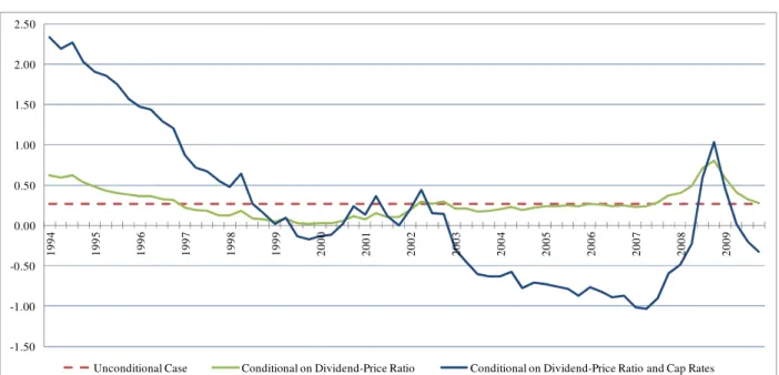
In the sections to follow we provide the reader with the results from the analysis, applying the dynamic allocation methodology described in this Section. More specifically, for each portfolio we have included two charts that show the time series of the portfolio weights of the two “basis” assets [expressions used: (18), (21), (24)], a table that shows the basic first and second moment statistics for the expanded portfolio, a table with the optimal portfolio weights of the augmented asset space [expressions used: (16), (18), (20), (23)] and a summarizing table of the portfolio performance.
4.3. Results of the Dynamic Portfolio Analysis with Quarterly Rebalancing
Exhibit 2: Stocks and R.E. “All Properties” Dynamic Portfolio Optimization (Unconditional and Conditional Portfolios with Quarterly Rebalancing)
Figure 2.1: Time Series of Portfolio Weights on Stocks
Figure 2.2: Time Series of Portfolio Weights on R.E. “All Properties” -2.00 -1.50 -1.00 -0.50 0.00 0.50 1.00 1.50 2.00 2.50 3.00 1 9 8 4 1 9 8 5 1 9 8 6 1 9 8 7 1 9 8 8 1 9 8 9 1 9 9 0 1 9 9 1 1 9 9 2 1 9 9 3 1 9 9 4 1 9 9 5 1 9 9 6 1 9 9 7 1 9 9 8 1 9 9 9 2 0 0 0 2 0 0 1 2 0 0 2 2 0 0 3 2 0 0 4 2 0 0 5 2 0 0 6 2 0 0 7 2 0 0 8 2 0 0 9
Unconditional Case Conditional on Dividend-Price Ratio Conditional on Dividend-Price Ratio and Cap Rates
-2.00 -1.00 0.00 1.00 2.00 3.00 4.00 5.00 1 9 8 4 1 9 8 5 1 9 8 6 1 9 8 7 1 9 8 8 1 9 8 9 1 9 9 0 1 9 9 1 1 9 9 2 1 9 9 3 1 9 9 4 1 9 9 5 1 9 9 6 1 9 9 7 1 9 9 8 1 9 9 9 2 0 0 0 2 0 0 1 2 0 0 2 2 0 0 3 2 0 0 4 2 0 0 5 2 0 0 6 2 0 0 7 2 0 0 8 2 0 0 9
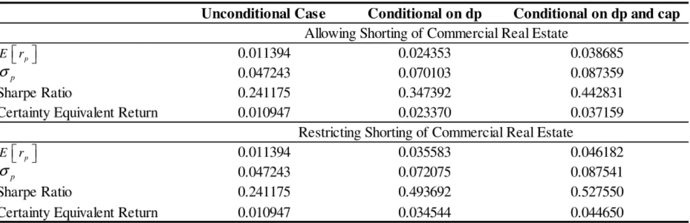
Table 2.1: Major First and Second Moment Statistics
Table 2.2: Optimal Portfolio Weights
Table 2.3: Dynamic Portfolio Performance
Asset S R.E. S-dp R.E.-dp S-cap R.E.-cap
0.017992 0.006655 -0.004154 -0.013054 0.010135 0.009290 0.082510 0.043877 0.085830 0.035473 0.084570 0.045650 Sharpe Ratio 0.218053 0.151664 -0.048394 -0.367989 0.119839 0.203500
Asset S R.E. S-dp R.E.-dp S-cap R.E.-cap
S 1.000000 0.185825 0.045493 -0.006098 -0.122552 -0.077165 R.E. 1.000000 -0.060296 0.050983 -0.051200 -0.553929 S-dp 1.000000 0.290012 -0.621519 -0.148331 R.E.-dp 1.000000 -0.162190 -0.137489 S-cap 1.000000 0.352786 R.E.-cap 1.000000
Return, Volatility and Sharpe Ratio of "Basis" and "Conditional" Portfolio Asse ts
Correlation Matrix of Portfolio Assets
[ ]
i E r i σ Stocks R.E. 0.871828 — 0.586544 0.463154 — — 0.859254 -1.301297 — 1.499485 — 0.286200 0.508612 0.296939 0.473687 —Conditional on dp and cap Conditional on dp Unconditional Case -1.074407 0.933634 S x% S dp x% − S cap x% − . . R E dp x% − . . R E cap x% − . . R E x%
Restricting Shorting of Commercial Real Estate 0.011394
0.047243 0.070103 0.087359
0.024353 0.038685
0.037159
Sharpe Ratio 0.241175 0.493692 0.527550
Certainty Equivalent Return 0.010947 0.034544 0.044650
0.011394 0.035583 0.046182
0.047243 0.072075 0.087541
0.241175 0.347392 0.442831
Conditional on dp
Unconditional Case Conditional on dp and cap
Allowing Shorting of Commercial Real Estate
Certainty Equivalent Return 0.010947
Sharpe Ratio 0.023370 p E r p σ p E r p σ
Exhibit 3: Stocks and R.E. Apartment Dynamic Portfolio Optimization (Unconditional and Conditional Portfolios with Quarterly Rebalancing)
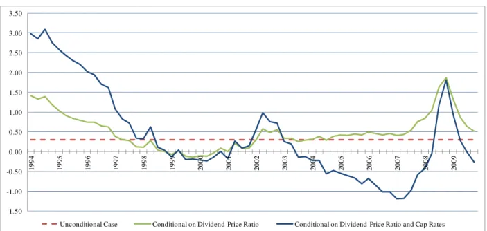
Figure 3.1: Time Series of Portfolio Weights on Stocks
Figure 3.2: Time Series of Portfolio Weights on R.E. Apartment -1.50 -1.00 -0.50 0.00 0.50 1.00 1.50 2.00 2.50 1 9 9 4 1 9 9 5 1 9 9 6 1 9 9 7 1 9 9 8 1 9 9 9 2 0 0 0 2 0 0 1 2 0 0 2 2 0 0 3 2 0 0 4 2 0 0 5 2 0 0 6 2 0 0 7 2 0 0 8 2 0 0 9
Unconditional Case Conditional on Dividend-Price Ratio Conditional on Dividend-Price Ratio and Cap Rates
-3.00 -2.00 -1.00 0.00 1.00 2.00 3.00 4.00 5.00 1 9 9 4 1 9 9 5 1 9 9 6 1 9 9 7 1 9 9 8 1 9 9 9 2 0 0 0 2 0 0 1 2 0 0 2 2 0 0 3 2 0 0 4 2 0 0 5 2 0 0 6 2 0 0 7 2 0 0 8 2 0 0 9
Table 3.1: Major First and Second Moment Statistics
Table 3.2: Optimal Portfolio Weights
Table 3.3: Dynamic Portfolio Performance
Asset S R.E. S-dp R.E.-dp S-cap R.E.-cap
0.015030 0.017185 -0.011410 -0.010269 0.013995 0.009011 0.086030 0.045118 0.110394 0.058516 0.081503 0.050998 Sharpe Ratio 0.174712 0.380882 -0.103355 -0.175496 0.171715 0.176697
Asset S R.E. S-dp R.E.-dp S-cap R.E.-cap
S 1.000000 0.133788 0.167570 0.252729 -0.037577 -0.187480 R.E. 1.000000 0.263950 0.426161 -0.252709 -0.359911 S-dp 1.000000 0.436184 -0.691200 -0.262944 R.E.-dp 1.000000 -0.301678 -0.147555 S-cap 1.000000 0.318281 R.E.-cap 1.000000
Return, Volatility and Sharpe Ratio of "Basis" and "Conditional" Portfolio Asse ts
Correlation Matrix of Portfolio Assets
[ ]
i E r i σ Stocks R.E. — -1.377659 -1.128597 — — 0.883890 — — 0.799177 1.332134 1.651428 2.083799 — 0.173866 0.604269 0.266058 0.268787 0.204847Unconditional Case Conditional on dp Conditional on dp and cap
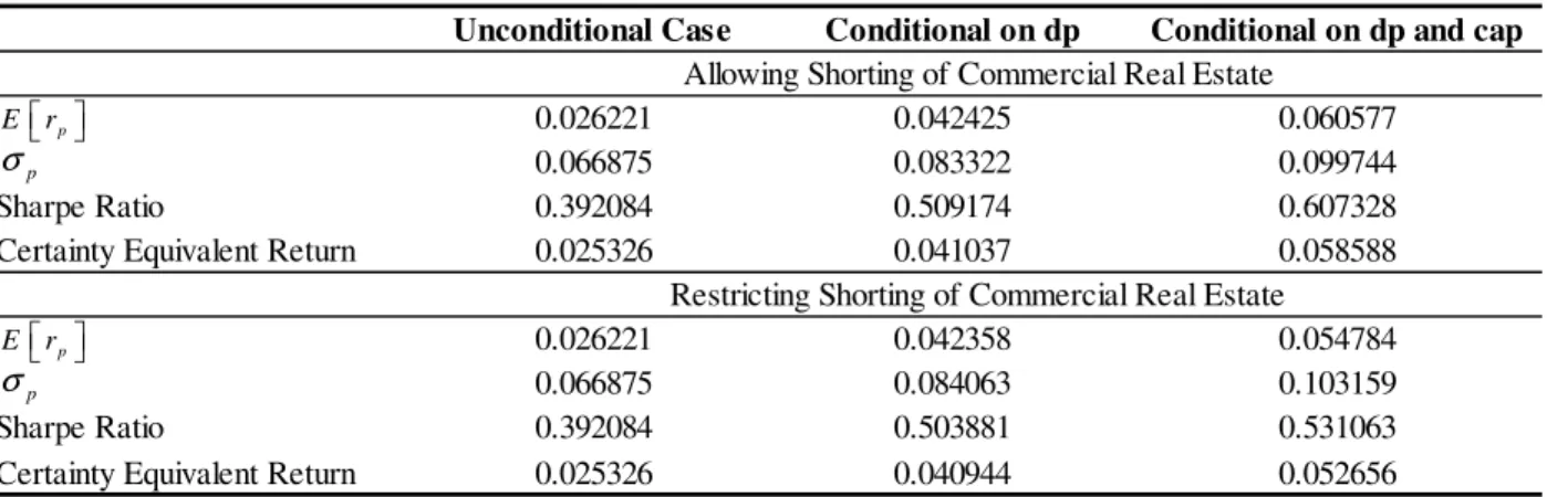
S x% S dp x% − S cap x% − . . R E dp x% − . . R E cap x% − . . R E x% Sharpe Ratio 0.392084 0.503881 0.531063
Certainty Equivalent Return 0.025326 0.040944 0.052656
Restricting Shorting of Commercial Real Estate
0.066875 0.084063 0.103159
0.026221 0.042358 0.054784
0.066875 0.083322 0.099744
Sharpe Ratio 0.392084 0.509174 0.607328
Certainty Equivalent Return 0.025326 0.041037 0.058588
Unconditional Case Conditional on dp Conditional on dp and cap
Allowing Shorting of Commercial Real Estate
0.026221 0.042425 0.060577 p E r p σ p E r p σ
Exhibit 4: Stocks and R.E. Industrial Dynamic Portfolio Optimization (Unconditional and Conditional Portfolios with Quarterly Rebalancing)
Figure 4.1: Time Series of Portfolio Weights on Stocks
Figure 4.2: Time Series of Portfolio Weights on R.E. Industrial -1.50 -1.00 -0.50 0.00 0.50 1.00 1.50 2.00 2.50 3.00 3.50 1 9 9 4 1 9 9 5 1 9 9 6 1 9 9 7 1 9 9 8 1 9 9 9 2 0 0 0 2 0 0 1 2 0 0 2 2 0 0 3 2 0 0 4 2 0 0 5 2 0 0 6 2 0 0 7 2 0 0 8 2 0 0 9
Unconditional Case Conditional on Dividend-Price Ratio Conditional on Dividend-Price Ratio and Cap Rates
-4.00 -3.00 -2.00 -1.00 0.00 1.00 2.00 3.00 4.00 1 9 9 4 1 9 9 5 1 9 9 6 1 9 9 7 1 9 9 8 1 9 9 9 2 0 0 0 2 0 0 1 2 0 0 2 2 0 0 3 2 0 0 4 2 0 0 5 2 0 0 6 2 0 0 7 2 0 0 8 2 0 0 9
Table 4.1: Major First and Second Moment Statistics
Table 4.2: Optimal Portfolio Weights
Table 4.3: Dynamic Portfolio Performance
Asset S R.E. S-dp R.E.-dp S-cap R.E.-cap
0.015030 0.014058 -0.011410 -0.018013 0.016335 0.010409 0.086030 0.056489 0.110394 0.082989 0.084045 0.064111 Sharpe Ratio 0.174712 0.248871 -0.103355 -0.217057 0.194358 0.162354
Asset S R.E. S-dp R.E.-dp S-cap R.E.-cap
S 1.000000 0.186425 0.167570 0.345068 -0.079308 -0.265670 R.E. 1.000000 0.377090 0.392704 -0.324303 -0.682864 S-dp 1.000000 0.563814 -0.732877 -0.362355 R.E.-dp 1.000000 -0.342130 -0.593581 S-cap 1.000000 0.422885 R.E.-cap 1.000000
Return, Volatility and Sharpe Ratio of "Basis" and "Conditional" Portfolio Asse ts
Correlation Matrix of Portfolio Assets
[ ]
i E r i σ Stocks R.E. — -1.242635 -0.895767 — — 0.616064 — — 0.906579 0.719029 0.839149 1.268901 — 0.445469 0.892207 0.297519 0.499072 0.419238Unconditional Case Conditional on dp Conditional on dp and cap
S x% S dp x% − S cap x% − . . R E dp x% − . . R E cap x% − . . R E x% Sharpe Ratio 0.274008 0.298905 0.385052
Certainty Equivalent Return 0.013656 0.026323 0.038237
Restricting Shorting of Commercial Real Estate
0.051797 0.093974 0.105035
0.014193 0.028089 0.040444
0.051797 0.087395 0.098215
Sharpe Ratio 0.274008 0.396518 0.505124
Certainty Equivalent Return 0.013656 0.033126 0.047682
Unconditional Case Conditional on dp Conditional on dp and cap
Allowing Shorting of Commercial Real Estate
0.014193 0.034654 0.049611 p E r p σ p E r p σ
Exhibit 5: Stocks and R.E. Office Dynamic Portfolio Optimization (Unconditional and Conditional Portfolios with Quarterly Rebalancing)
Figure 5.1: Time Series of Portfolio Weights on Stocks
Figure 5.2: Time Series of Portfolio Weights on R.E. Office -3.00 -2.00 -1.00 0.00 1.00 2.00 3.00 4.00 1 9 9 4 1 9 9 5 1 9 9 6 1 9 9 7 1 9 9 8 1 9 9 9 2 0 0 0 2 0 0 1 2 0 0 2 2 0 0 3 2 0 0 4 2 0 0 5 2 0 0 6 2 0 0 7 2 0 0 8 2 0 0 9
Unconditional Case Conditional on Dividend-Price Ratio Conditional on Dividend-Price Ratio and Cap Rates
-3.00 -2.00 -1.00 0.00 1.00 2.00 3.00 4.00 5.00 1 9 9 4 1 9 9 5 1 9 9 6 1 9 9 7 1 9 9 8 1 9 9 9 2 0 0 0 2 0 0 1 2 0 0 2 2 0 0 3 2 0 0 4 2 0 0 5 2 0 0 6 2 0 0 7 2 0 0 8 2 0 0 9
Table 5.1: Major First and Second Moment Statistics
Table 5.2: Optimal Portfolio Weights
Table 5.3: Dynamic Portfolio Performance
Asset S R.E. S-dp R.E.-dp S-cap R.E.-cap
0.015030 0.014324 -0.011410 -0.013963 0.016676 0.009305 0.086030 0.044327 0.110394 0.044334 0.088459 0.049061 Sharpe Ratio 0.174712 0.323144 -0.103355 -0.314946 0.188515 0.189664
Asset S R.E. S-dp R.E.-dp S-cap R.E.-cap
S 1.000000 0.157020 0.167570 0.127588 -0.085438 -0.065658 R.E. 1.000000 0.089806 0.461992 -0.096325 -0.304750 S-dp 1.000000 0.324724 -0.714967 -0.120002 R.E.-dp 1.000000 -0.132915 -0.302438 S-cap 1.000000 0.356509 R.E.-cap 1.000000
Return, Volatility and Sharpe Ratio of "Basis" and "Conditional" Portfolio Asse ts
Correlation Matrix of Portfolio Assets
[ ]
i E r i σ Stocks R.E. — -1.322216 -1.552409 — — -0.304212 — — 1.222042 1.234449 1.903514 2.032296 — 0.179860 0.898094 0.272811 0.111047 0.034330Unconditional Case Conditional on dp Conditional on dp and cap
S x% S dp x% − S cap x% − . . R E dp x% − . . R E cap x% − . . R E x% Sharpe Ratio 0.337583 0.526252 0.525002
Certainty Equivalent Return 0.020362 0.041474 0.054972
Restricting Shorting of Commercial Real Estate
0.062641 0.081323 0.109255
0.021146 0.042796 0.057359
0.062641 0.079141 0.102295
Sharpe Ratio 0.337583 0.546792 0.547177
Certainty Equivalent Return 0.020362 0.042021 0.053881
Unconditional Case Conditional on dp Conditional on dp and cap
Allowing Shorting of Commercial Real Estate
0.021146 0.043274 0.055974 p E r p σ p E r p σ
Exhibit 6: Stocks and R.E. Retail Dynamic Portfolio Optimization (Unconditional and Conditional Portfolios with Quarterly Rebalancing)
Figure 6.1: Time Series of Portfolio Weights on Stocks
Figure 6.2: Time Series of Portfolio Weights on R.E. Retail -2.00 -1.50 -1.00 -0.50 0.00 0.50 1.00 1.50 2.00 2.50 1 9 9 4 1 9 9 5 1 9 9 6 1 9 9 7 1 9 9 8 1 9 9 9 2 0 0 0 2 0 0 1 2 0 0 2 2 0 0 3 2 0 0 4 2 0 0 5 2 0 0 6 2 0 0 7 2 0 0 8 2 0 0 9
Unconditional Case Conditional on Dividend-Price Ratio Conditional on Dividend-Price Ratio and Cap Rates
-3.00 -2.00 -1.00 0.00 1.00 2.00 3.00 1 9 9 4 1 9 9 5 1 9 9 6 1 9 9 7 1 9 9 8 1 9 9 9 2 0 0 0 2 0 0 1 2 0 0 2 2 0 0 3 2 0 0 4 2 0 0 5 2 0 0 6 2 0 0 7 2 0 0 8 2 0 0 9