HAL Id: hal-02927266
https://hal.archives-ouvertes.fr/hal-02927266
Submitted on 8 Sep 2020
HAL is a multi-disciplinary open access
archive for the deposit and dissemination of
sci-entific research documents, whether they are
pub-lished or not. The documents may come from
teaching and research institutions in France or
abroad, or from public or private research centers.
L’archive ouverte pluridisciplinaire HAL, est
destinée au dépôt et à la diffusion de documents
scientifiques de niveau recherche, publiés ou non,
émanant des établissements d’enseignement et de
recherche français ou étrangers, des laboratoires
publics ou privés.
balance by incorporating SPITFIRE into the global
vegetation model ORCHIDEE – Part 1: simulating
historical global burned area and fire regimes
C. Yue, P. Ciais, P. Cadule, K. Thonicke, S. Archibald, B. Poulter, W. Hao, S.
Hantson, F. Mouillot, P. Friedlingstein, et al.
To cite this version:
C. Yue, P. Ciais, P. Cadule, K. Thonicke, S. Archibald, et al.. Modelling the role of fires in the
terrestrial carbon balance by incorporating SPITFIRE into the global vegetation model ORCHIDEE
– Part 1: simulating historical global burned area and fire regimes. Geoscientific Model Development,
European Geosciences Union, 2014, 7 (6), pp.2747-2767. �10.5194/gmd-7-2747-2014�. �hal-02927266�
www.geosci-model-dev.net/7/2747/2014/ doi:10.5194/gmd-7-2747-2014
© Author(s) 2014. CC Attribution 3.0 License.
Modelling the role of fires in the terrestrial carbon balance by
incorporating SPITFIRE into the global vegetation model
ORCHIDEE – Part 1: simulating historical global burned
area and fire regimes
C. Yue1,2, P. Ciais1, P. Cadule1, K. Thonicke3, S. Archibald4,5, B. Poulter6, W. M. Hao7, S. Hantson8,9, F. Mouillot10, P. Friedlingstein11, F. Maignan1, and N. Viovy1
1Laboratoire des Sciences du Climat et de l’Environnement, LSCE CEA CNRS UVSQ, 91191 Gif-Sur-Yvette, France 2Laboratoire de Glaciologie et Géophysique de l’Environnement, UJF, CNRS, Saint Martin d’Hères CEDEX, France 3Potsdam Institute for Climate Impact Research (PIK) e.V., Telegraphenberg A31, 14473 Potsdam, Germany 4CSIR Natural Resources and Environment, P.O. Box 395, Pretoria 0001, South Africa
5School of Animal, Plant and Environmental Sciences, University of the Witwatersrand, Johannesburg, Private Bag
X3,WITS, 2050, South Africa
6Institute on Ecosystems and Department of Ecology, Montana State University, Bozeman, MT 59717, USA 7US Forest Service, Rocky Mountain Research Station, Fire Sciences Laboratory, Missoula, MT, USA 8University of Alcalá, Department of Geography, Calle Colegios 2, Alcalá de Henares 28801, Spain
9Karlsruhe Institute of Technology, Institute of Meteorology and Climate research, Atmospheric Environmental Research,
82467 Garmisch-Partenkirchen, Germany
10IRD, UMR CEFE, 1919 route de mende, 34293 Montpellier CEDEX 5, France
11College of Engineering, Mathematics and Physical Sciences, University of Exeter, Exeter, EX4 4QE, UK Correspondence to: C. Yue (chao.yue@lsce.ipsl.fr)
Received: 15 February 2014 – Published in Geosci. Model Dev. Discuss.: 10 April 2014 Revised: 17 September 2014 – Accepted: 16 October 2014 – Published: 21 November 2014
Abstract. Fire is an important global ecological process that influences the distribution of biomes, with consequences for carbon, water, and energy budgets. Therefore it is impossi-ble to appropriately model the history and future of the ter-restrial ecosystems and the climate system without includ-ing fire. This study incorporates the process-based prognos-tic fire module SPITFIRE into the global vegetation model ORCHIDEE, which was then used to simulate burned area over the 20th century. Special attention was paid to the evaluation of other fire regime indicators such as season-ality, fire size and fire length, next to burned area. For 2001–2006, the simulated global spatial extent of fire agrees well with that given by satellite-derived burned area data sets (L3JRC, GLOBCARBON, GFED3.1), and 76–92 % of the global burned area is simulated as collocated between the model and observation, depending on which data set is used for comparison. The simulated global mean annual
burned area is 346 Mha yr−1, which falls within the range of 287–384 Mha yr−1as given by the three observation data sets; and is close to the 344 Mha yr−1by the GFED3.1 data when crop fires are excluded. The simulated long-term trend and variation of burned area agree best with the observation data in regions where fire is mainly driven by climate varia-tion, such as boreal Russia (1930–2009), along with Canada and US Alaska (1950–2009). At the global scale, the simu-lated decadal fire variation over the 20th century is only in moderate agreement with the historical reconstruction, pos-sibly because of the uncertainties of past estimates, and be-cause land-use change fires and fire suppression are not ex-plicitly included in the model. Over the globe, the size of large fires (the 95th quantile fire size) is underestimated by the model for the regions of high fire frequency, compared with fire patch data as reconstructed from MODIS 500 m burned area data. Two case studies of fire size distribution
in Canada and US Alaska, and southern Africa indicate that both number and size of large fires are underestimated, which could be related with short fire patch length and low daily fire size. Future efforts should be directed towards building con-sistent spatial observation data sets for key parameters of the model in order to constrain the model error at each key step of the fire modelling.
1 Introduction
Fire is an important process in the Earth system, that ex-isted long before the large-scale appropriation of natural ecosystems by humans (Bowman et al., 2009; Daniau et al., 2013). Fires have multiple biophysical and ecological con-sequences, and they are also an important source of atmo-spheric trace gases and aerosol particles (Langmann et al., 2009; van der Werf et al., 2010). By damaging some plant types and concurrently promoting others, fires play an impor-tant role in shaping vegetation structure and function (Bond et al., 2005; Pausas and Keeley, 2009). Fire changes the sur-face albedo, aerodynamic roughness, and the sensible and la-tent heat fluxes (Liu et al., 2005; Liu and Randerson, 2008). These fire-induced ecosystem changes could further influ-ence the surface energy budget and boundary-layer climate (Beck et al., 2011; Randerson et al., 2006; Rogers et al., 2013). In addition, gas and aerosol species emitted to the at-mosphere from biomass burning modify atmospheric com-position and the radiative forcing balance (Tosca et al., 2013; Ward et al., 2012). Fire aerosols also degrade air quality and cause increased health risk (Marlier et al., 2013). Thus fire process and biomass burning emissions need to be included in the Earth system models, which are often used to inves-tigate the role of fire in past, present and future biophysical and biogeochemical processes.
The type of fire model embedded in global vegetation models has evolved from simple fire hazard models (Thon-icke et al., 2001) to the current state-of-the-art process-based fire models (Andela et al., 2013; Kloster et al., 2010; Lass-lop et al., 2014; Li et al., 2013; Pfeiffer et al., 2013; Pren-tice et al., 2011) and empirical models with optimisation by observation (Knorr et al., 2014; Le Page et al., 2014). The majority of fire models explicitly simulate ignitions from natural and human sources, fire propagation, fuel combus-tion and vegetacombus-tion mortality, ideally at daily or even finer time steps. Recently, Pfeiffer et al. (2013) have incorporated multi-day burning, “coalescence” of fires and interannual lightning variability in the LPJ-LMfire model. Li et al. (2013) incorporated social and economic factors in the human igni-tion scheme. Lasslop et al. (2014) investigated the model sen-sitivity to the climate forcing and a number of spatial param-eters. Evaluation of fire models in these studies at the global scale has mainly focused on models’ capability in broadly re-producing the large-scale distribution of fire activity during
the past decade as revealed by satellite observations. Less at-tention was paid to the simulation of long-term historical fire trend and variation, and fire regimes, which may include the number, size and intensity of fires – essential variables gov-erning fire–climate–vegetation feedbacks (Archibald et al., 2013; Barrett et al., 2011; Hoffmann et al., 2012).
It is well known that across all fire-prone ecosystems, the magnitude and trend of burned area depend strongly on large fire events that represent only a low fraction in total number of fires (Kasischke and Turetsky, 2006; Keeley et al., 1999; Stocks et al., 2002). These large fires have profound impacts on landscape heterogeneity (Schoennagel et al., 2008; Turner et al., 1994), biological diversity (Burton et al., 2008) and may also induce a higher rate of carbon emissions compared with small fires (Kasischke and Hoy, 2012). Besides, the so-cial and economic consequences of extreme large fires are more severe (Richardson et al., 2012). In some ecosystems, past climate warming was shown to have increased the oc-currence of large fires (Kasischke et al., 2010; Westerling et al., 2006), and fire regimes were projected to even further deviate from historical range given the future climate change (Pueyo, 2007; Westerling et al., 2011). Given the importance of these large fires, it is essential that we should evaluate the ability of fire models to simulate their occurrence.
In this study, we have incorporated the SPITFIRE fire model (Thonicke et al., 2010) into the global land surface model ORCHIDEE (Krinner et al., 2005). This allowed us to simulate global fire activity during the 20th century, and to perform an in-depth model evaluation. In present study, we focus on evaluating the ORCHIDEE-SPITFIRE model per-formance in simulating fire behaviours and regimes, includ-ing ignitions, fire spread rate, fire patch length, fire size distri-bution, fire season and burned area. Quantification of fire car-bon emission as a component of the terrestrial carcar-bon balance will be presented in a companion paper (Part 2). Specifically, the objectives of the present study are: (1) to evaluate simu-lated burned area using multiple data sets including that from satellite observation, government fire agency, and historical reconstruction over the 20th century (Sects. 3.1, 3.2, 3.3, 3.4. 3.5); (2) to compare simulated fire size distribution with ob-servations, in order to investigate especially the model’s abil-ity to simulate large fire occurrence (Sect. 3.6); and (3) to examine potential sources of model error in order to iden-tify future research need and potential model improvements (Sect. 4.2).
2 Data and methods
2.1 Model description
The processes and equations of the fire model SPITFIRE, as described by Thonicke et al. (2010), were implemented in the vegetation model ORCHIDEE (Krinner et al., 2005). The SPITFIRE model operates on a daily time step, consistent
with the STOMATE sub-module in ORCHIDEE, which sim-ulates vegetation carbon cycle processes (photosynthates al-location, litterfall, litter and soil carbon decomposition). The major processes within SPITFIRE are briefly described be-low with applicable minor modifications (see Thonicke et al., 2010 for more detailed description).
2.1.1 Daily potential ignition
Daily potential ignition includes ignitions from lightning and human activity. Remotely sensed lightning flashes (Cecil et al., 2012) were obtained from the High Resolution Monthly Climatology of lightning flashes by the Lightning Imaging Sensor–Optical Transient Detector (LIS/OTD) (http://gcmd. nasa.gov/records/GCMD_lohrmc.html). The LIS/OTD data set provides annual mean flashes over 1995–2000 on a 0.5◦ grid at monthly time step. This single annual data was re-peated each year throughout the simulation. Following Pren-tice et al. (2011), the proportion of lightning flashes that reach the ground with sufficient energy to ignite a fire is set as 0.03. This value differs from that in the original SPIT-FIRE model as implemented in LPJ-DGVM (Thonicke et al., 2010); there a cloud-to-ground (CG) flashing ratio of 0.2 was used, followed by a further ignition efficiency of 0.04.
To estimate potential ignitions by humans, the original Eqs. (3) and (4) in Thonicke et al. (2010) were modified for the purpose of unit adjustment, as below:
IH=PD × 30.0 × e−0.5× √
PD×a(ND)/10 000 (1)
where IH is the daily ignition number (1 day−1km−2),
PD is population density (individuals km−2). The parameter
a(ND) (ignitions individual−1day−1)represents the
propen-sity of people to produce ignition events; and is a spatially explicit parameter as in Thonicke et al. (2010) (Supplement Fig. S1).
2.1.2 Daily fire numbers
Daily fire numbers are derived by scaling the potential igni-tions (which include human and lightning igniigni-tions) with the fire danger index (FDI), which is derived by comparing sim-ulated daily fuel moisture to a plant functional type (PFT) dependent moisture of extinction. All fires with a fireline in-tensity less than 50 kW m−1are assumed unable to propagate and are suppressed as stated by Thonicke et al. (2010). 2.1.3 Daily mean fire size
Daily mean fire size is calculated by assuming an elliptical shape of fire, with the major axis length being the product of fire spread rate and daily fire active burning time (i.e. the time that fires actively burn during that day). Fire spread rate is obtained using the Rothermel equation (Rothermel, 1972; Wilson, 1982). Fire active burning time is modelled to in-crease as a logistic function of daily fire danger index, with a
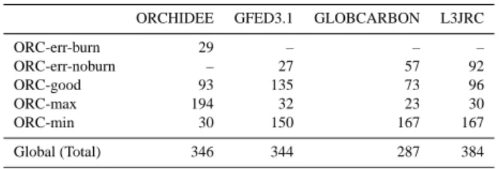
Table 1. Mean annual burned area (Mha yr−1)for 2001–2006 for different ORCHIDEE simulation quality flags as shown in Fig. 4.
ORCHIDEE GFED3.1 GLOBCARBON L3JRC
ORC-err-burn 29 – – – ORC-err-noburn – 27 57 92 ORC-good 93 135 73 96 ORC-max 194 32 23 30 ORC-min 30 150 167 167 Global (Total) 346 344 287 384
maximum of 241 min (4 h). Fire frontline intensity is calcu-lated following Byram (1959), as a product of fuel heat con-tent, fuel consumption, and fire spread rate. Note that over a grid cell of 0.5 degree, the model simulates a set of homoge-neous fires with all their characters (including fire size) being identical among each other, i.e. the model represents the tem-poral but not the spatial heterogeneity over a given grid cell. Daily grid cell burned area is calculated as the product of fire number and mean fire size.
2.1.4 Fire-induced tree mortality
Fire-induced tree mortality is determined from the combined fire damage of tree crown and cambium. Crown damage de-pends on the fraction of tree crown that is affected by crown scorch, which further depends on tree crown length, tree height and fire flame height. Fire flame height is derived from surface fire intensity. Cambial damage depends on fire res-idence time and a prescribed PFT-dependent critical time. Note that SPITFIRE simulates only crown scorch, but not active crown fires that could propagate through crown fire spread.
2.1.5 Fire carbon emissions
Fire carbon emissions include emissions from surface fuel and crown combustion. Surface fuels are divided into four classes (1, 10, 100 and 1000 h), whose designation in terms of hours describes the order of magnitude of time required to lose (or gain) 63 % of its difference with the equilib-rium moisture content under defined atmospheric condi-tions (Thonicke et al., 2010). Fuel combustion complete-ness is simulated as a function of daily fuel moisture, with a smaller fraction of fuel being consumed at higher fuel moisture. Crown fuel consumption is related to the frac-tion of crown that is scorched by fire flame. The values of all PFT-dependent parameters follow Table 1 in Thonicke et al. (2010).
2.2 Further modifications made to the SPITFIRE equations
Fires in dry climate regions are limited by the availability of fuel on the ground (Krawchuk and Moritz, 2010; Prentice et al., 2011; Van der Werf et al., 2008b). This constraint is
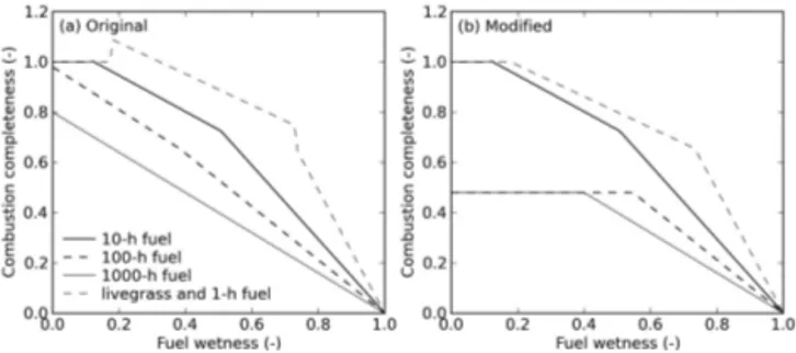
im-Figure 1. Surface-fuel combustion completeness as a function of fuel wetness in (a) original SPITFIRE model by Thonicke et al. (2010) and (b) as modified in the present study, taking the trop-ical forests as an example. The combustion of live grass biomass is assumed to follow that of 1 h dead fuel.
plicitly included in SPITFIRE equations, because fire occur-rence is limited by a fireline intensity of 50 kW m−1.
How-ever during model testing, we found that this threshold is not enough to limit fires in low-productivity regions (with mod-elled annual net primary productivity of 0–400 g C m−2yr−1, corresponding to an annual precipitation of 0–400 mm); and too much burned area was simulated for arid and semi-arid regions (see Supplement Fig. S2). Following Arora and Boer (2005), we therefore introduced a new factor that lim-its the ignition efficiency, depending on the availability of ground fuel. Ignition efficiency varies linearly between zero when ground fuel is lower than 200 g C m−2, to unity when ground fuel is above 1000 g C m−2. Here, ground fuel in-cludes aboveground litter and live biomass for grassland PFTs and aboveground litter only for tree PFTs.
The equations for surface fuel combustion complete-ness given by Thonicke et al. (2010) follow Peterson and Ryan (1986), which allow combustion completeness to de-crease with increasing fuel wetness and level out when fuel wetness drops below a threshold (Fig. 1). During model testing, we found that because fuel wetness frequently ap-proaches zero, simulated fuel combustion completeness is much higher than field experiment values as reported by van Leeuwen et al. (2014). We therefore modified the maximum combustion completeness for fuel classes of 100 and 1000 h to be the same as mean combustion completeness by van Leeuwen et al. (2014) depending on different biomes (PFTs). This biome-dependent maximum combustion completeness is 0.48 for tropical broadleaf evergreen and seasonal forests, 0.45 for temperate forest, 0.41 for boreal forest, 0.85 for grassland, and 0.35 for cropland. These values are based on a preliminary version of results by van Leeuwen et al. (2014). 2.3 Input data set and the simulation protocol
The 6-hourly climate fields used to drive the model were from the CRU-NCEP data set (http://dods.extra.cea.fr/store/ p529viov/cruncep/V4_1901_2012/readme.htm). Population density for the 20th century was retrieved from the
His-tory Database of the Global Environment (HYDE) as compiled by the Netherlands Environmental Assessment Agency (http://themasites.pbl.nl/tridion/en/themasites/hyde/ download/index-2.html). From 1850 until 2005, the HYDE gridded data are available for the beginning of each decade and for 2005. Annual data were linearly interpolated within each decade, and further re-gridded to 0.5◦ resolution. For 2006–2009, population density was set as constant at the 2005 value.
A three-step simulation protocol was used. For the first two steps, the atmospheric CO2 was fixed at the
pre-industrial level (285 ppm) and climate forcing data of 1901–1930 were repeated in loop. The first step was a without-fire spin-up from bare ground lasting for 200 years (including a 3000-year run of soil-only processes to speed up the equilibrium of mineral soil carbon). The second step was a fire-disturbed spin-up lasting for 150 years, with fire being switched on to account for fire disturbances in the pre-industrial era. Fire ignitions from human activity were in-cluded in the fire-disturbed spin-up, with the human popu-lation density being fixed at 1850 level. This procedure as-sumes that the model reached an equilibrium state under con-ditions of pre-industrial atmospheric CO2 and climate and
fire disturbance.
The third step was a transient simulation from 1850 to 2009 with increasing atmospheric CO2, climate change,
and varying human population density. The climate data used for the transient simulation of 1850–1900 were a re-peat of 1901–1910, for the sake of stability. Before en-tering the transient simulation, the mineral soil carbon stock was verified to vary within 0.1 % (with a slight global carbon sink of 0.13 Pg C yr−1 and a negligible
an-nual trend of 0.003 Pg C yr−1 during the last 50 years of
the fire-disturbed spin-up, excluding all crops, for which fires are not simulated). For the current simulation, the vegetation dynamics module of ORCHIDEE was turned off, i.e. the simulation used a static current-day vegetation distribution map (converted into the 13-PFT map in OR-CHIDEE based on the IGBP 1 km vegetation map, http: //webmap.ornl.gov/wcsdown/dataset.jsp?ds_id=930), and no land cover change was included. This static land cover could affect the model–observation agreement in terms of long-term trend and variation of burned area. Land cover change has double effects on burned area: fires used for land cover change contribute directly to burned area; and the indirect effect depends on fire frequencies of the land cover types be-fore and after the land cover change.
Fires on croplands are not simulated in ORCHIDEE, even though the model has two PFTs that approximately represent C3 and C4 crops (but without realistic species-specific phe-nology). Magi et al. (2012) show that cropland fire seasons differ significantly from those of natural fires, warranting a special treatment of cropland fires in global fire modelling (Li et al., 2012). Cropland fires make up a rather small pro-portion of the total global amount in terms of both burned
area (4.3 % according to the GFED3.1 data set) and car-bon emissions (less than 2 % according to GFED3.1), given that the “small” fires (Randerson et al., 2012) are not for-mally included and recommended in the GFED data set (http://www.globalfiredata.org/data.html).
Further, deforestation fires are not explicitly simulated. Evidence shows that deforestation fires occur during the “time window” when climate is dry enough to allow com-plete burning of deforested fuels (Van der Werf et al., 2008a). We expect the simulated daily fire danger index (i.e. an in-dicator of suitable climate conditions for burning) is able to partly capture this “fire climate window” that is necessary for deforestation fires to happen. Thus the model is able to im-plicitly account for some deforestation fire activity in tropi-cal and subtropitropi-cal forests, but not for all of them, because of the use of a static land cover map. Preliminary analysis shows that the model could capture ∼ 67 % of the deforested area by fires as given by the GFED3.1 data for closed-canopy forests in the region of 20◦S–20◦N for 2000–2005 (2.7 Mh yr−1vs. 4.0 Mha yr−1) (Fig. S3), with the seasonal variation being moderately represented (Fig. S4).
2.4 Data sets used to evaluate model performance
Several data sets were prepared and used to compare simu-lated burned area and fire regimes with various observations. 2.4.1 Spatially gridded burned area data
Satellite-derived burned area data
The GFED3.1 data set provides monthly burned area data at 0.5◦resolution for 1997–2009 with global coverage (Giglio
et al., 2010). The GFED3.1 burned area was mainly gen-erated using MODIS imagery with additional images from TRMM VIRS and ERS ATSR. The fire carbon emissions were also provided which are model simulation results by applying a modified version of the CASA model (van der Werf et al., 2010).
L3JRC data set provides daily global burned area data at 1 km resolution for April 2000 to March 2007; these data were generated from the 1 km SPOT VEGETATION satellite imagery (Tansey et al., 2008). This data set was assembled at 0.5◦resolution at monthly time step for use in the present study.
GLOBCARBON burned area data was produced
from a combination of SPOT VEGETATION and
ERS2–ATSR2/ENVISAT AATSR data as one of the four land products of the ESA GLOBCARBON initiative (Plummer et al., 2007). Global burned area data were provided at monthly resolution with four different spatial resolutions (1 km/10 km/0.25◦/0.5◦) covering 1998–2007.
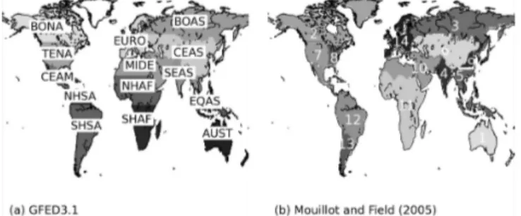
Figure 2. The regional breakup of the globe according to (a) the GFED3.1 data set: BONA, boreal North America; TENA, temperate North America; CEAM, Central America; NHSA, Northern Hemi-sphere South America; SHSA, Southern HemiHemi-sphere South Amer-ica; EURO, Europe; MIDE, Middle East; NHAF, Northern Hemi-sphere Africa; SHAF, Southern HemiHemi-sphere Africa; BOAS, boreal Asia; CEAS, central Asia; SEAS, Southeast Asia; EQAS, equa-torial Asia; AUST, Australia and New Zealand. And (b) Mouillot and Field (2005): (1) Australia and New Zealand; (2) boreal North America; (3) boreal Russia; (4) India; (5) Southeast Asia; (6) cen-tral Asia; (7) USA (western Mississippi); (8) USA (eastern Missis-sippi); (9) East Asia; (10) Middle East and northern Africa; (11) Africa (sub-Saharan); (12) central South America; (13) southern South America; (14) Europe.
Historical burned area reconstruction for the 20th century
To evaluate the simulated burned area for the 20th century, historical burned area data were used. These data, which cover the period 1900–2000, were compiled by Mouillot and Field (2005) at 1◦ resolution and monthly time step (here-after referred to as the Mouillot data). The data were gener-ated by first synthesising the burned area information from published data at national or regional scale for the periods of the 1980s or 1990s, further interpolated spatially at the global scale at 1◦ resolution using the available satellite-derived active fire distribution. Then national fire statistics, historical land-use practices and other fire-relevant quantita-tive information (such as tree ring reconstruction) were used to build the historical fire temporal trend to interpolate his-torical burned area.
When comparing the burned area given by GFED3.1 and the Mouillot data for their overlapping period of 1997–2000, the global total burned area given by Mouillot and Field (2005) is 52 % higher than GFED3.1 with signif-icant regional discrepancies. As the satellite-derived data is considered to be more reliable than the national or regional statistical data at a large spatial scale, a bias correction was performed on the Mouillot data. We calculated the ratio of burned area by the Mouillot data to GFED3.1 for 1997–2009 for each region (Fig. 2b) and also the globe. This ratio was then applied to correct for each decade of the burned area data in the Mouillot data set.
Note that the regional breakdowns of the globe by GFED3.1, and Mouillot and Field (2005) are different (Fig. 2). For comparison of burned area for the 20th century, the regional breakdown by Mouillot and Field (2005) was adopted as it is based on maximum temporal stability (er-ror consistency), a highly important factor when comparing long-term data.
2.4.2 Fire patch data
Alaskan and Canadian fire management agencies have main-tained historical fire monitoring for a relatively long time (dating back to the 1950s). The historical fire information for the US Alaska was retrieved from the Alaska Intera-gency Coordination Center (AICC, http://afsmaps.blm.gov/ imf_firehistory/imf.jsp?site=firehistory). The fire informa-tion for Canada was from the Canadian Wildland Fire Infor-mation System (http://cwfis.cfs.nrcan.gc.ca/ha/nfdb). These data sets contain information on fire location, fire size (burned area), fire cause, and for some fires, the fire report and out date. Please note that in these two data sets fires with all sizes are included.
Archibald et al. (2010) classified the MCD45A1 500 m MODIS fire burned area data into individual fire patches for southern Africa (Africa south to the Equator). This fire patch information includes location and patch size (with minimum fire size of 0.25 km2). The fire patch data for Canada and US Alaska, and southern Africa are used to evaluate simulated fire size distribution.
2.4.3 Fire season length and the 95th quantile fire size
The global fire season length and the 95th quantile fire size data are provided by Archibald et al. (2013). The fire season length was quantified as the number of months required to reach 80 % of the annual burned area using GFED3.1 data. The MCD45A1 burned area product at 500 m resolution was used to derive the individual fires by applying a flood-fill al-gorithm, and the 95th quantile fire size in each grid cell was extracted to represent the size of large fires.
2.5 Methods to compare model simulation with observation
2.5.1 Metrics used to evaluate modelled burned area against GFED3.1 data
As the GFED3.1 data is most widely used by the fire mod-elling community, the model results are evaluated against GFED3.1 data for 1997–2009. Three aspects were examined: mean annual burned area, interannual variability (IAV) and seasonality in burned area. The evaluation was done for each GFED3.1 region (Fig. 2).
For the model error in terms of mean annual burned area (BA), we use the relative difference:
EBA=
BAmodel−BAGFED
BAGFED
(2) where BAmodel is the simulated burned area averaged over
1997–2009, and BAGFED is GFED3.1 mean annual burned
area for the same period. The similarity in IAV (Sinterannual)
is estimated by the correlation coefficient of the two lin-early detrended annual burned area time series by model and GFED3.1 data. Finally, the seasonality similarity (Sseason)is
given by: Sseason= 12 X i=1 min(frac_modeli,frac_GFEDi) (3)
where frac_modeli and frac_GFEDi are the fraction of
burned area for the ith month relative to the annual burned area (i.e. monthly BA normalised by the annual BA).
Sseasonrepresents the overlapping area of the two normalised
monthly BA series and indicates the fraction of burned area in temporal coincidence. The statistical significance of
Sseasonwas examined by using a bootstrapping method. First,
normalised monthly BA from all 14 regions by the model and GFED3.1 data were pooled together. Second, 100 000 pairs of monthly normalised BA were randomly sampled from the pooled data in order to derive a probability distribution function (PDF) of Sseason. Third, the single-sided probability
(p value) that the calculated Sseasonis from random
distribu-tion is obtained for each region, and a p value less than 0.05 indicates the model could moderately capture the seasonality of burning (i.e. significantly different from a random distri-bution).
The peak fire month, which is defined as the month with maximum monthly burned area, is compared between the model and GFED3.1 data. The difference between simulated and observed peak month is quantified by the following in-dex, after Prentice et al. (2011):
D2= " 1 − X j =1,n Ajcos θj/ X j =1,n Aj !# . 2 (4)
where θj is the angle between vectors representing the
simu-lated and observed peak fire month (with January to Decem-ber resembling 1 to 12 on a clock), n is the total numDecem-ber of grid cells and Aj is the burned area by GFED3.1 data.
Ac-cording to Eq. (4), the value of D2 is zero when simulated
peak month is perfectly in phase with the observation, 0.5 if the timing is off by 3 months in either direction, and one (the maximum) if the timing is off by 6 months.
2.5.2 Concatenate simulated consecutive daily fire events into multi-day fire patches
The fire patch data for Canada and US Alaska, and southern Africa contain fires that span multiple days. In the model,
fires are simulated as independent daily events with the active burning time being limited to 4 h (i.e. all fires have the same size; they start and extinguish within the same day). Pfeiffer et al. (2013) introduced a mechanism to allow fires to span multiple days under suitable weather conditions. Inspired by their study, we developed an approach to concatenate fires during consecutive days into “multi-day fire patches”. The size of each “multi-day fire patch” is the cumulative daily fire size during its persistence time. This allows the modelled “multi-day fire patch size” to be compared to observations. For clarity, the period of multiple days that a fire spans is hereafter referred to as “fire patch length”.
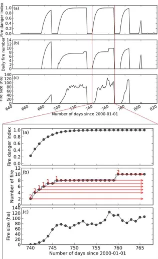
The approach to concatenate independent daily fires into multi-day fire patches is illustrated in Fig. 3, which shows simulated daily fire number and fire size for a 0.5◦grid cell in northern Africa for the fire season of October 2001 to April 2002. Fires occur in different consecutive-day periods, i.e. when simulated FDI remains above zero, and when fuel amount and fire intensity exceed the given thresholds. In the example in Fig. 3, the model simulated five such periods, each spanning a different number of days. Within each pe-riod, with the increase of FDI (i.e. advancing into more suit-able fire weather, shown in subplot a), the simulated daily number of fires (subplot b) and the mean fire size (subplot c) increased as well.
Figure 3 lower panel illustrates in detail how separate daily fires were concatenated into fire patches for the period of Day 740–766 (since 1 January 2000). Rather than viewing fires on a given day as being independent from those of pre-vious days, we now consider part of these fires as “persisting” from previous days and part of these fires as new patches. For example, on Day 741, four fires were originally simulated to start and extinguish within this day (with the exact same fire size). We now consider that two of these four fires persisted from the previous day, i.e. the two fire patches staring on Day 740. We then consider that the other two fires of Day 741 were new fire patches initiated on this day. Similarly, the five fires originally simulated on Day 742 are now considered as:
– two extended from the two fire patches of Day 740 (which already persisted into Day 741);
– two extended from the two fire patches of Day 741;
– one new fire patch started at this day.
Following this approach, fires simulated in all following days were identified either as extending from fire patches of previous days, or as new fire patches. As such, the total num-ber of fire patches is equal to the maximum daily fire numnum-ber during this period. In the example of Fig. 3 lower panel, ten fire patches were extracted from Day 740 to 766 (as indicated by the numbers and arrows in red in the subplot b):
Figure 3. Schematic diagram showing the concatenation of fires within consecutive days into multi-day fire patches. An example is given for a 0.5◦grid cell in northern Africa for the fire season from October 2001 to April 2002. Upper panel: fires in different consecutive-day periods as simulated by the model. Lower panel: zooming for the period of Day 740–766 since 1 January 2000. Ten different fire patches were extracted from fires in this period. The number of fire patches and their persistence time were indicated by the numbers and arrows in red in the subplot (b), respectively. Refer to Sect. 2.5.2 for detailed explanations.
– two fire patches extended from Day 740 to 766;
– two extended from Day 741 to 766;
– one extended from Day 742 to 766;
– ...
– the last two fire patches extended from Day 760 to 766.
The size for each fire patch was the cumulative daily fire size during its persistence time. The procedure illustrated in Fig. 3 was repeated for all the land grid cells (excluding those with less than 10 days of fire occurrence) over 1997–2009, to generate the “multi-day fire patches” over the globe.
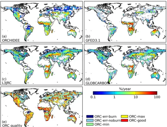
Figure 4. Mean annual burned fraction (in percentage) over 2001–2006 (a) as simulated by ORCHIDEE, and by the satellite-derived burned area data sets: (b) GFED3.1, (c) L3JRC and (d) GLOBCARBON. The subplot (e) shows for each grid cell the quality flag of ORCHIDEE-simulated burned fraction in comparison with observation data sets. ORC-err-burn, where ORCHIDEE shows burning but the other three observation data sets do not; ORC-err-noburn, where at least two of the three observation data sets do show burning, but ORCHIDEE does not; ORC-min, where ORCHIDEE simulates lower burned fraction than the other three data sets; ORC-max, where ORCHIDEE simulates higher burned fraction; ORC-good, where ORCHIDEE-simulated burned fraction falls within the range given by the three observation data sets. When calculating the minimum and maximum burned fraction of the observation data sets, an arbitrary tolerance margin of 25 % was applied around the min/max value to take into account the observation uncertainty.
3 Results
3.1 Comparison of model simulation to satellite observation for the spatial and temporal pattern of burning
Figure 4 shows the spatial distribution of mean annual burned fraction by the model and the three satellite-derived data sets (GFED3.1, GLOBCARBON, L3JRC) for 2001–2006. L3JRC and GLOBCARBON show similar spatial patterns of burning, which is different from the GFED3.1 data. Gen-erally, L3JRC and GLOBCARBON have less burned area in the Southern Hemisphere than GFED3.1 (see also Fig. 5a), with smaller spatial extent of burning in the savanna systems in Africa and Australia. By contrast, in the middle to high latitudes of the Northern Hemisphere, L3JRC and GLOB-CARBON show more burned area than GFED3.1. All three data sets capture the grassland burning in central and eastern Asia.
ORCHIDEE coupled with SPITFIRE is generally able to reproduce the spatial distribution and magnitude of
satellite-observed burned fraction. The simulated mean annual global burned area for 2001–2006 is 346 Mha yr−1, which falls
within the range of 287–384 Mha yr−1 given by the
satel-lite observation data, and close to the 344 Mha yr−1 by the
GFED3.1 data set when crop fires are excluded.
Fires in grassland-dominated systems are well captured by the model, including steppe fires in central and eastern Asia, savanna fires in northern Africa, northern Australia and cen-tral to east South America. Two regions could be identified where model simulation is different from all the three ob-servation data sets. One is the woodland savanna (miombo) in southern Africa, where burned area is underestimated by the model (simulated annual burned fraction is ∼ 4 %, but 14–24 % is observed). The other is western and central con-tinental US (dominated by C3 and C4 grass in the land-cover map used by ORCHIDEE) where fires are overestimated (simulated annual fraction is ∼ 6%, but 1–2 % is observed). For the fires in high-latitude (> 45◦N) boreal forest, sparsely
forested area and tundra, the magnitude of burned fraction by ORCHIDEE falls between that found in the GFED3.1 and in the L3JRC/GLOBCARBON data sets (Fig. 4).
Figure 5. (a) Latitudinal distribution of burned area (Mha yr−1) according to GFED3.1 (blue), ORCHIDEE (thick black), GLOB-CARBON (orange) and L3JRC (green). Data are shown for the mean annual value for 2001–2006. (b) Annual burned area time se-ries for different data sets.
The simulation pixels are divided into five classes accord-ing to their simulation quality, as shown in Fig. 4. Table 1 shows the mean burned area for each category and data set. The grid cells with burning collocated between model and observation data (labelled as good, max, ORC-min in Fig. 4) cover the majority of global burned area (76–92 % depending on different data sets), indicating that the model can reproduce the major spatial extent of burning. However, discrepancy still remains, in that 50 % of the mod-elled global burned area is classified as ORC-max (i.e. over-estimation of burned fraction by the model), whereas obser-vation data sets have half of the global burned area labelled as ORC-min (i.e. underestimation of burned fraction by the model).
Figure 4 also illustrates the lower burned area found in L3JRC and GLOBCARBON in comparison with GFED3.1 for the Southern Hemisphere and subtropical Northern Hemisphere, in contrast to the higher burned area in the middle-to-high latitude region in the Northern Hemisphere. The simulated latitudinal distribution of burned area gen-erally falls within the minimum–maximum range of the three observation products. Exceptions are the regions of
∼5–15◦S and 30–40◦N, corresponding to the underesti-mated burning in southern African savanna and the overesti-mate in western and central US, discussed above. The annual time series of burned area are shown in Fig. 5b. The cor-relation coefficient between ORCHIDEE and the GFED3.1 data is highest (0.48; linearly detrended correlation coeffi-cient of 0.59), compared to that of 0.26 between
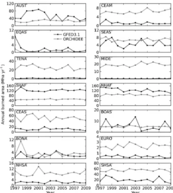
GLOBCAR-Figure 6. Annual burned area by ORCHIDEE (grey) and GFED3.1 data (black) for 1997–2009 for the 14 GFED regions.
BON and the GFED3.1; and −0.59 between L3JRC and the GFED3.1.
3.2 Model evaluation against GFED3.1 burned area data
The simulated burned area for 1997–2009 is evaluated against the GFED3.1 data for each region in terms of mean annual burned area, and similarity in interannual variability and seasonality (see metrics in Sect. 2.5). The results are pre-sented in Table 2; and the annual burned areas for different regions are shown in Fig. 6.
The model error for annual burned area (BA) is highest for the Middle East (MIDE, by a factor of 41.9, occupying 0.1 % vs. 5.6 % of global BA by GFED3.1 vs. ORCHIDEE) and lowest for boreal Asia (BOAS, by a factor of −0.1, oc-cupying 1.6 % vs. 1.4 % of global BA). The model underesti-mates burned area in the three biggest fire regions (Northern Hemisphere Africa, Southern Hemisphere Africa and Aus-tralia, together occupying 86 % vs. 46.8 % of global BA) by on average 45.6 %. Prominent model overestimation is found in central Asia (CEAS, by a factor of 3.8, occupying 3 % vs. 14.9 % of global BA), and Southern Hemisphere South America (SHSA, by a factor of 1.6, occupying 5.5 % vs. 15.7 % of global BA).
The correlation coefficient for the linearly detrended global annual burned area between ORCHIDEE and GFED3.1 is 0.59, indicating that the model moderately cap-tures the IAV of burned area (although it fails to reproduce
Table 2. Model error characterisation in comparison with the GFED3.1 data for 1997–2009. EBA, the model error of mean annual burned area in relative to the GFED3.1 data; Sinterannual, the correlation coefficient of linearly detrended annual simulated and GFED3.1 burned area
series; Sseason, the seasonal similarity of burned area by the model and the GFED3.1 data (see Sect. 2.5 for the definition of each metrics).
Region (in Fig. 2a) EBA Sinterannual S∗season Burned area by GFED3.1 Percentage of the global total Percentage of the global total Peak fire month
(ha yr−1) burned area (GFED3.1) burned area (ORCHIDEE) (GFED3.1, model)
BONA 0.6 0.53 0.7 2.1 0.6 1.0 (7,7) TENA 18.1 0.52 0.75 1.3 0.4 7.4 (8,7) CEAM 4.4 0.55 0.63 1.2 0.3 1.8 (5,4) NHSA 3.2 −0.12 0.96 2.1 0.6 2.6 (2,2) SHSA 1.8 0.41 0.71 19.2 5.5 15.7 (8,8) EURO 4.9 0.01 0.86 0.4 0.1 0.7 (8,8) MIDE 41.9 0.22 0.73 0.4 0.1 5.6 (8,6) NHAF −0.3 0.01 0.59 125.1 35.8 24.9 (12,12) SHAF −0.6 0 0.68 123.2 35.2 14.4 (8,6) BOAS −0.1 0.43 0.55 5.6 1.6 1.4 (7,7) CEAS 3.8 0.08 0.75 10.5 3.0 14.9 (8,7) SEAS 0.5 −0.12 0.52 4.7 1.3 2.0 (3,4) EQAS −0.8 0.97 0.73 1.7 0.5 0.1 (9,9) AUST −0.5 0.37 0.75 52.4 15.0 7.5 (10,11) ∗
A bootstrapping method was used to derive a probability distribution function of Sseasonby randomly sampling from the normalised monthly burned area of GFED3.1 and the model for 100 000 times. The bold number indicates that the Sseasonis not significantly different from a randomised monthly distribution of burned area at a significant level of 0.05.
the 1998 El Niño peak burning), because errors are compen-sated among regions (Fig. 5b). On regional scale, the model performs best at regions where the IAV of burned area is known to be mainly driven by climate, such as boreal North America (BONA), boreal Asia (BOAS), and equatorial Asia (EQAS). However, the model performs rather poorly for re-gions where burned area shows little IAV such as Africa (NHAF and SHAF, see also Fig. 6), or the burned area is unrealistically simulated by the model (such as TENA and MIDE). For most regions the model captures the fire season-ality rather well (Table 2), with Sseason being significantly
different from that of a randomly distributed seasonality, ex-cept in NHAF, BOAS and SEAS.
3.3 Fire and precipitation relationship
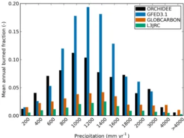
The model captures well the empirical relationship between burned area and precipitation found in tropical and sub-tropical regions (Fig. 7; see also Prentice et al., 2011; Van der Werf et al., 2008b). In low-precipitation regions (< 400 mm yr−1), the climate is favourable for fire but burn-ing is limited by the available fuel. In contrast, regions with higher precipitation (> 2000 mm yr−1) always support suf-ficient fuel amount but fires are limited by the duration of dry season when fires can occur. Burned area is maximal for regions with intermediate precipitation and productivity (Krawchuk and Moritz, 2010).
Maximum burning occurs around an annual precipita-tion of 1000 mm according to model simulaprecipita-tion, com-pared to 1200 mm by GFED3.1, and 1400 mm by the GLOBCARBON and L3JRC data sets. GLOBCARBON and L3JRC show the lowest burning in this tropical/subtropical belt, followed by the model simulation, with the burned area by GFED3.1 being the highest. The fire and pre-cipitation relationship was further divided into four sub-regions of America, Africa, Asia and Australia following
Figure 7. Burned fraction distribution as a function of annual pre-cipitation according to: the model simulation (black); GFED3.1 (blue); GLOBCARBON (orange); and L3JRC (green) for the tropi-cal and subtropitropi-cal regions (35◦S–35◦N). The annual precipitation data are from CRU data and binned in 200 mm intervals.
Van der Werf et al. (2008b) and the results are shown in Supplement Fig. S5. The model–observation agreement in fire–precipitation pattern is moderate in Africa and Australia, but low-precipitation fires are overestimated in America and Asia.
3.4 Peak fire month and fire season length
The spatial distributions of fire peak months by ORCHIDEE and GFED3.1 are compared in Fig. 8. The spatial pattern of simulated peak fire month is in general agreement with GFED3.1 data. The model simulation gives D2 as 0.3,
Figure 8. Spatial pattern of the peak fire month by (a) ORCHIDEE and (b) GFED3.1 data over 1997–2009. Only grid cells with fire collocated in both data sets are shown.
Figure 9. Fire season length (months) by (a) Archibald et al. (2013) derived from GFED3.1 data, and (b) ORCHIDEE simulation for 1997–2009.
by on average 2 months. At regional scale, simulated peak fire months for most regions are within 1 month of those by GFED3.1 data, except MIDE and SHAF (see the far right-hand column of Table 2). Refer to Supplement Fig. S6 for more detailed information of modelled and observed sea-sonal pattern of burning for different GFED3.1 regions.
Figure 9 compares simulated fire season length with the GFED3.1-derived fire season length from Archibald et al. (2013). The spatial pattern of fire season length by model simulation agrees well with that given by Archibald et al. (2013), with fire season length lasting 1–3 months in boreal regions, and 4–7 months in semi-arid grasslands and savannas. The fire season length in eastern Africa, South Africa, Botswana, Namibia, Argentina and Mexico is over-estimated by the model by 2–4 months; and underover-estimated in southeast Brazil by 1–2 months.
3.5 Long-term trends of burned area during the 20th century
Over the 20th century, the historical trend of modelled global total burned area generally follows the Mouillot re-construction data (Mouillot and Field, 2005) as corrected by GFED3.1 data (see Sect. 2.4.1), with increasing burned area after the 1930s until the 1990s–2000s, after which global burned area began to decrease (Fig. 10). However, the inter-decadal variability of burned area is underestimated. Region-ally, simulated decadal burned area agrees relatively well with the Mouillot data in boreal Russia (beginning from the 1930s), although the observation data is subject to great un-certainty, especially before the 1950s (Mouillot and Field, 2005). The simulated burned area also agrees well with fire agency data for Canada and US Alaska (Supplement Fig. S7). The correlation coefficient for annual BA between model and fire agency data is 0.44 after 1950, and 0.57 be-tween model and Mouillot data, when the observation data are considered to be more reliable. This reflects the model capability to capture fire variability driven by climate varia-tion relatively well.
The model fails, however, to capture burned area varia-tion for regions where fires from changed land cover likely played a bigger role in the earlier 20th century according to the Mouillot data (Mouillot and Field, 2005); for example, in Australia and New Zealand, USA and southern South Amer-ica, mainly because the static land cover was used in the sim-ulation. Strong model–observation disagreement also occurs for regions where the implementation of modern fire preven-tion has drastically reduced the burned area, as occurred in the 1960s in boreal North America, because the general im-plicit inclusion of human suppression on ignitions in Eq. (1) on the global scale does not accommodate regional unique-ness.
3.6 Compare simulated fire size with observation
In this section we compare the simulated fire size distribution against observation over two regions: Canada and US Alaska combined, and southern Africa. The number and size of re-constructed “multi-day fire patches” by the model were used (see Sect. 2.5.2). For both simulated and observed fires, all fires within the test region were pooled together. Fires were
Figure 10. The annual burned area for 1901–2009 as simulated by ORCHIDEE (grey bar), reported by the Mouillot data (Mouillot and Field, 2005, black bar), and by GFED3.1 data (dashed white bar). Data are shown for the mean values over each decade for 1901–2000, and for 2001–2005 (2000 sA) and 2006–2009 (2000 sB). Refer to Sect. 2.4.1 for the correction of the Mouillot data by using GFED3.1 data.
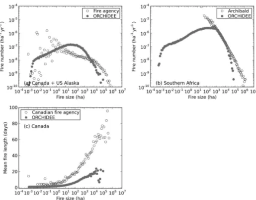
Figure 11. Fire size distribution as simulated by the model and derived from (a) fire agency data for US Alaska and Canada, and (b) MODIS 500 m burned area data by Archibald et al. (2010) for southern Africa. The horizontal axis indicates fire size (ha) and the vertical axis indicates the corresponding number of fires (in units of ha−1yr−1)for the given fire size. (c) The fire patch size and corresponding mean fire patch length (in unit of days) by the model simulation and Canadian fire agency data (using only the fire patches for which fire report and out date are available).
binned according to fire patch size in an equal logarithmic distance manner (with the minimum–maximum size range being divided into 100 bins). The mean annual number of fires on an area basis for each bin was calculated. For the fire patches in Canada for which fire start date and fire out date were reported, fire length was calculated and compared with model simulation as well.
Figure 11 shows the fire size and the corresponding num-ber of fires for each size bin over US Alaska and Canada, and southern Africa. The modelled fire size distribution reaches a maximum at intermediate fire sizes. This is because when the climate is less favourable for fire occurrence, both num-ber of fires and fire size are limited (corresponding to the low fire size end in Fig. 11a and 11b). While the size and num-ber of fires could be large during the period when climate is dry and large fires are possible (corresponding to the high fire size end in Fig. 11a and 11b), the frequency of high-fire period itself might be rare. The similar pattern is shown by the fire agency data of Canada and US Alaska, but not by the satellite-derived fire patch data in southern Africa, which might be due to that the minimum fire size (25 ha) is limited by the satellite resolution there. However, for both regions, the frequency and size of extreme large fires were underes-timated by the model. Further comparison of fire lengths for Canada (Fig. 11c) reveals that the model underestimated fire length by as much as 60 days for the extreme large fires.
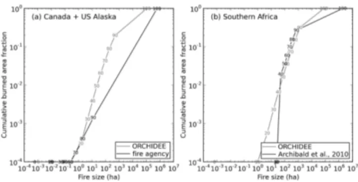
We further calculated the cumulative fraction of total burned area by fires below a given quantile of fire size (the minimum size, every tenth quantile from 10th to 90th quan-tile, and the maximum size) (Fig. 12). According to observa-tion, in boreal Canada and US Alaska, the total burned area is mainly dominated by a few large fires, with the top 10 % of fires (90th quantile to the maximum size) accounting for 99.8 % of the total burned area. By contrast, the same group of fires (i.e. the highest 10 % large fires) account for ∼ 80 % of the simulated total burned area, with the remaining being accounted for by many small fires. For southern Africa, the model distribution follows rather relatively well of the obser-vation. The top 30 % of fires (70th quantile to the maximum size) make up 90 % of the total burned area by satellite data and 85 % by the model simulation.
Figure 13 compares the simulated 95th quantile fire size with the global observation by satellite. According to observation, fires with biggest fire size (500–10 000 km2)
are grassland-dominated fires in central and eastern Asia, African savanna and northern Australia, which are followed by fires in Russian and Alaskan boreal forest (and sparsely forested area) or tundra, and savanna-woodland fires in Africa and central South America (50–500 km2). Fires in the rest of the world are relatively small (< 50 km2). In terms of spatial fire size distribution, the model could re-produce the biggest fires in grassland-dominated systems in central and eastern Asia (200–1000 km2), northern Australia (50–200 km2), as well as fires in Russian boreal forest (and sparsely forested area) or tundra (50–200 km2; note that
tun-Figure 12. Fire size and the corresponding cumulative fraction of the total burned area by fires below a given fire size for (a) Canada & US Alaska, and (b) southern Africa. Data are shown for a series of equally distanced 10th quantile fire sizes. Numbers in the curves show the location of every 10th quantile fire size from 0th quantile (the minimum fire size) to 100th quantile (the maximum fire size).
dra is treated as C3 grassland in the model), but fire size for these regions is generally smaller than observation by up to one magnitude. The fire size in central South America tends to be underestimated, and overestimated in western to cen-tral US. Fire size for the rest of the world is comparable be-tween model and the observation, with general small fire size (< 50 km2)and low fire frequency.
4 Discussion
4.1 General model performance
The SPITFIRE module was first presented by Thonicke et al. (2010). It was later adapted in the Land surface Processes and exchanges (LPX) model by Prentice et al. (2011), no-tably with the removal of ignition sources created by humans, and further by Pfeiffer et al. (2013) and Lasslop et al. (2014). Pfeiffer et al. (2013) developed a scheme to allow fire span of multiple days and fire coalescence, explored the role of lightning interannual variability in the model, and included terrain effects on fire at a broad scale. Lasslop et al. (2014) investigated model sensitivity to climate forcing and to the spatial variability of a number of fire relevant parameters. In the current study, the SPITFIRE module was fully integrated into the global process-based vegetation model ORCHIDEE for the first time. Simulated burned area, fire season and fire patch size distribution were evaluated in a comprehensive way against observation for the recent period (1997–2009), and against reconstructed burned area for the 20th century.
The simulated global mean annual burned area for 2001–2006 agrees with the satellite observation data and is most close to the GFED3.1 data. The model could moder-ately capture the interannual variability in burned area as re-vealed by GFED3.1 data with the exception of the peak burn-ing of 1998, probably because the deforestation and tropi-cal peat fires in the 1997–98 El Niño event (Van der Werf
et al., 2008a) were not represented. Model–observation dis-crepancy remains at a regional scale, with underestimation mainly in the savanna of Africa and Australia, and overes-timation in central Asia, Middle East, the temperate North America, and Southern Hemisphere South America.
The model can reproduce the maximal burned area for the intermediate range of precipitation for tropical and subtrop-ical regions (35◦S–35◦N) (also shown by Prentice et al., 2011; Van der Werf et al., 2008b). For boreal regions where climate plays a dominant role in driving the temporal varia-tion of burned area, simulated burned area generally agrees well with the historical reconstruction data (boreal Russia for 1930–2009) and government fire agency data (US state of Alaska and Canada for 1950–2009), indicating that the model is capturing the climate as a driver of fire. However, on the global scale, because fire trend is determined by multiple factors including climate, land-use practice and fire suppres-sion (Mouillot and Field, 2005), simulated burned area trend only agrees moderately well with the reconstruction data for the 20th century, given that the static land cover and the sim-ple human ignition equation were used in the model. 4.2 Potential sources of systematic errors
Fire is a complex, regional process that involves diverse di-mensions of vegetation, climate and human activity (Bow-man et al., 2009). Uncertainties in all these factors will con-tribute to the overall uncertainty in simulated fire activities. Because SPITFIRE simulates fire occurrence through a com-plex chain that includes factors from potential ignition to fire climate, to fire spread rate and fire size and tree mortality, identifying contributions of each modelling step to the ulti-mate error in simulated fire regime is problematic. A com-plete error analysis involving all model parameters is beyond the scope of this study, but following sections are intended to serve as preliminary investigation of model errors.
4.2.1 Ignition sources
On the global scale, due to the limitation of fire by fuel load on the arid and semi-arid regions, modelled annual burned area is more closely related to the total fire numbers rather than the fire danger index (Fig. S8). This might lead to spec-ulation that the potential ignition source is the first identi-fied source of error for simulated burned area. One possible error in ignition is that potential lightning ignitions are not suppressed by human presence in densely populated areas, which cause lightning-ignited fires being overestimated. We have tested this possibility by applying a population density-dependent human suppression of lightning-ignited fires fol-lowing Li et al. (2012), and the result showed that part of the overestimation of burned fraction in western US and central South America could be reduced (Figs. 4 and S9), but the burned area in Africa and over the whole globe were further underestimated.
Figure 13. Map of the 95th quantile fire patch size (km2)as given by (a) Archibald et al. (2013) from MCD45A1 MODIS 500 m burned area data, and (b) ORCHIDEE simulation.
Published fire models (Kloster et al., 2012; Li et al., 2012; Pechony and Shindell, 2009; Venevsky et al., 2002) gener-ally include ignitions from lightning and human sources, to-gether with explicit or implicit human suppression of fires. However, one common challenge is to properly calibrate ig-nition parameters. One option is to use active fire counts (as in case of Li et al., 2012; Pechony and Shindell, 2009), but fire counts are not exactly real fire numbers, because a sin-gle widespread fire could be seen as many fire counts and the burned area per hotspot may vary by an order of magnitude depending on vegetation composition (Hantson et al., 2013). Simulated burned area on the global scale might be compara-ble with the satellite observation data. However, very little is known on how this agreement was achieved; nor on whether each step of the modelling process was correctly captured, or if the ultimate agreement in burned area is mainly thanks to error compensation among different steps. Two recent mod-elling studies (Lasslop et al., 2014; Yang et al., 2014) used some scaling factor to adjust either directly burned area or the ignitions to match simulated global burned area with ob-servation.
Pfeiffer et al. (2013) argued that interannual lightning vari-ability was critical for their model to capture the trend and interannual variation of burned area, especially for regions where burned area is dominated by lightning fires such as boreal forests in Alaska and Canada. Currently, a single data set of monthly lightning flashes was repeated each year in our model. However, we have tested the possibility to include the interannual lightning variability by following their approach. The historical lightning variability during the 20th century was reconstructed by using the convective potential
avail-able energy (CAPE) output variavail-able from the 20th Cen-tury Reanalysis Project (http://portal.nersc.gov/project/20C_ Reanalysis/), following Eq. (1) on page 649 of Pfeiffer et al. (2013). A test simulation was run for 1901–2009 over the whole globe with the variable lightning input. We found that shifting from repeated lightning data to CAPE-derived data decreased the Pearson correlation coefficient between sim-ulated decadal burned area and the Mouillot reconstruction for half of the 14 regions and for the globe, but increased the correlation for other regions. Over 1997–2009 with ob-servation data by GFED3.1 more credible than the 20th cen-tury reconstruction, using the CAPE-derived data decreased the Pearson correlation coefficient between annual simulated burned area and GFED3.1 for the globe and for most of the regions. This surprising result could be due to the fact that model internal errors may compensate for possible benefits of using the CAPE-derived data, or because CAPE-derived lightning data does not reflect the real lightning variability everywhere. For more detailed results and discussions, refer to the Sect. S2 of the Supplement.
4.2.2 Fire number, size and fire patch length
The comparison of simulated “multi-day fire patches” against the observation in Canada and US Alaska, and southern Africa shows that the model underestimated the frequency and size of extreme large fires. Given that an-nual burned area in US Alaska and Canada is slightly overestimated by the model (2.8 Mha yr−1 by model dur-ing 1960–2009 against 2.2 Mha yr−1 by fire agency and 1.9 Mha yr−1by the Mouillot data, also refer to Fig. S7 in the
Supplement), the total number of (the small- and medium-sized) fires must be overestimated (i.e. making compensation for the too small fire size). However, the compensation by fire numbers does not occur for southern Africa, where, given the underestimation of large fire size, the total burned area remains underestimated (Fig. 4, Table 2). Over the globe, despite the fact that the model correctly identifies some re-gions where large fires occur (mainly with grassland fraction higher than ∼ 70 % by the land cover map used in the model), the large fire size remains underestimated – by approximately one magnitude (Fig. 13).
The fire size of reconstructed “multi-day fire patches” is defined as the cumulative daily fire size over the correspond-ing fire patch length, and the underestimation of large fires could be due to underestimation in either fire patch length or daily fire size (i.e. fire patch size grows too slowly over its length). The comparison of simulated fire length with fire agency data in Canada suggests that model generally underestimated fire length. For fires larger than 10 000 ha, the underestimation is as large as 40–60 days. Given sim-ilar underestimation of large fire sizes in other ecosystems that are characterised by large-size fires (Fig. 13), the fire length underestimation in Canada is likely to happen else-where, though this could not be completely verified mainly
because of the lack of fire length observation across the world (the satellite-derived fire size data by Archibald et al., 2010, 2013 used in this study does not include the corresponding fire length yet).
In Pfeiffer et al. (2013), fires were simulated to span mul-tiple days and extinguish when the cumulative precipitation exceeds some threshold, with the daily fire size remaining limited by 241 min. There is one significant difference be-tween our approach and theirs. In Pfeiffer et al. (2013), fires starting on a given day are always considered as “new fires” to be added on the existing fire count on the previous day. The number of fires over a given grid cell thus accumulates each day as the time advances in a period suitable for fire occurrence. In our model, fires are originally simulated as independent events within individual days (because they are assumed to start and extinguish during the same day). To al-low the comparison of simulated fire size against observa-tions, these independent fires were concatenated (regrouped) into fire patches that span a different number of days. We made the concatenation by assuming fires at a given day ei-ther persist from the previous days or are actual new fire patches. Thus the number of reconstructed fire patches by our approach is the maximum daily fire number during the consecutive days of burning.
This difference in accounting for fire patches arose from the different approaches to handle ignitions in the two mod-els, in particular ignitions by lightning activities, because an-thropogenic ignitions were excluded in Pfeiffer et al. (2013). Pfeiffer et al. (2013) simulated lightning-ignited fires by fi-nally dropping the physical meaning of the number of light-ning flashes in the input data. This information was only used to obtain an all-or-nothing answer, allowing either a sin-gle fire over the whole 0.5-degree grid cell or no fire at all. However, the number of cloud-to-ground lightning flashes retained its physical meaning in our approach, and was scaled by the simulated FDI and fuel-limiting ignition efficiency to derive a daily number of fires. As no validation information was provided regarding fire number and fire size in Pfeiffer et al. (2013), it is unclear which approach yields results closer to observations. Overall, it remains challenging to develop a proper approach to represent the heterogeneous fire patches, and the growth of each individual patch in grid-based models (Jones et al., 2009).
4.2.3 Daily fire size, active burning time and fire spread rate
The underestimation of large fire sizes in Canada is partly due to underestimation of fire patch length. A closer compar-ison of Fig. 11a and 11c suggests that, while fire length was underestimated by a factor of 2–3 for fires between 104and 105ha, given the same fire number (shown as the vertical axis of Fig. 11a), the fire size was underestimated by roughly an order of magnitude (10 times). This implies the (mean) daily fire size is likely underestimated as well (roughly 3–5 times).
Within the model, daily fire size is determined by daily fire active burning time and fire spread rate. Evidence shows that wildfires display a characteristic diurnal cycle, with the most active time being around midday and early afternoon when the humidity is at a minimum and wind speeds are higher (Mu et al., 2011; Pyne et al., 1996; Zhang et al., 2012). Out-side this active burning time, fires could persist but propa-gate at a rather low speed (especially at night) or even turn into smouldering and burn with flame later again when the weather is feasible. For extremely large fires, the active burn-ing period could be longer because these fires often occur when the fuel is extremely dry as a consequence of extended drought weather. Currently, this active burning time is sim-ulated to exponentially increase with the fire danger index (i.e. indicator of daily fire weather) with a maximum time of 241 min. This limit might not be feasible for all ecosys-tems and fire sizes; however, a full exploration of this issue is currently limited by the scarcity of observations.
A global map of simulated 95th quantile fire spread rate is provided in the Supplement (see Fig. S10). Li et al. (2012) compiled fire spread information from the literature and re-ported typical fire spread rates of 12 m min−1for grasslands, 10.2 m min−1 for shrubs, 9 m min−1for needle-leaved trees and 6.6 m min−1 for other trees. The simulated fire spread in grasslands in central and eastern Asia (20–40 m min−1)
is much higher than the observed range. Considering that daily fire sizes are likely to be underestimated, the limit of 241 min maximum daily active burning time might be too short to correctly simulated large fire sizes in these grass-land ecosystems. By contrast, simulated fire spread rate in savanna vegetation (1–5 m min−1)is lower than the reported
value (10–12 m min−1), and this could help to explain the
underestimation of fire size and the broad underestimation of burned area in this region.
Fire spread in the northern high-latitude boreal forest, sparsely forested area and tundra is modelled to be ex-tremely high (> 10 m min−1). This is mainly because herba-ceous plants in these regions are simulated as C3 grasslands in the model with relatively low bulk density. However, the likely high daily burned area due to the high fire spread rate was compensated by simulated short fire patch length in the model (Fig. 11c), so that the simulated burned area for the re-gion of 50–75◦N agrees well with GFED3.1 data (Fig. 5a). Pfeiffer et al. (2013) proposed to relate the grass fuel bulk density with the annual sum of degree days over 5◦C. We have tested their approach and found that this new approach decreased the simulated burned area for the high-latitude re-gion (50–70◦N) and for the globe, and thus was not included
in the current version of model.
To gain more insights into the model’s behaviour, the sim-ulated 95th quantile fire patch size was related with other parameters (grassland fraction, fuel bulk density). As shown in Fig. S11, the size of large fires exponentially depends on the fire spread rate. The fire spread rate is very sensitive to the fuel bulk density and grass fraction beyond some
thresh-old (e.g. fire spread rate surges when grass coverage exceeds
∼70 %), with the fuel bulk density being inversely depen-dent on the grass fraction. Thus the simulated fire size could be sensitive to the land cover map (especially grass fraction) used in the simulation. Besides, as a static land cover map is used in our simulation, the grassland fraction is not al-lowed to vary as a response to fire disturbance. Thus a full fire–climate–vegetation feedback is limited, and this could probably help to explain the underestimation of fire size. 4.2.4 Influence of fire–climate–vegetation feedback
In the current simulation, the dynamic vegetation module of ORCHIDEE was switched off and a static land cover map was used. Tree mortality was affected by fire-induced tree damage, but tree coverage within a given grid cell was static and not allowed to vary with fire occurrence. A test simula-tion has been done for Southern Hemisphere Africa follow-ing the same simulation protocol as in Sect. 2.3 but with the dynamic vegetation module being switched on, in order to in-vestigate the simulated fire behaviour with dynamic vegeta-tion. Figure S12 compares the simulated annual burned area, grass and tree coverage change and the fire danger index for 1901–2009 with the model in dynamic and static vegetation modes.
In dynamic vegetation mode, the simulated burned area suddenly begins to increase around 1965, in response to the increased fire danger index. The increase in fire activity fur-ther increases the grass coverage and reduces tree coverage, causing a positive feedback to finally induce a peak of burned area around 1975, after which the burned area decreases. In static vegetation mode, the simulated burned area shows a similar peak in response to the peak in the fire danger in-dex, however, with a much smaller peak of burned area than that simulated in dynamic vegetation mode because of the lack of fire–vegetation–climate feedback. Simulated burned area by both simulations is still lower than that given by the GFED3.1 data for the period of 1997–2009, although the peak burned area in the dynamic vegetation mode is com-parable with GFED3.1 data.
This test indicates that including the
fire–climate–vegetation feedback could improve the simulation when the climate is favourable for fire occur-rence. At the same time, it also suggests that other factors like climate, and the model mechanisms determining the competitiveness of trees versus grass, might also play a role in the error of fire modelling.
4.2.5 Potential error sources for regional bias
Given that burned area is simulated in the model as a result of several sequential steps (lightning and human ignitions, fire number and fire size distribution, fire patch length, daily fire size, daily active burning time and fire spread rate), and the scarcity of global coverage observation data, we are not able