HAL Id: hal-00648708
https://hal.inria.fr/hal-00648708
Submitted on 6 Dec 2011
HAL is a multi-disciplinary open access
archive for the deposit and dissemination of
sci-entific research documents, whether they are
pub-lished or not. The documents may come from
teaching and research institutions in France or
abroad, or from public or private research centers.
L’archive ouverte pluridisciplinaire HAL, est
destinée au dépôt et à la diffusion de documents
scientifiques de niveau recherche, publiés ou non,
émanant des établissements d’enseignement et de
recherche français ou étrangers, des laboratoires
publics ou privés.
A Nash-game approach to joint image restoration and
segmentation
Moez Kallel, Rajae Aboulaich, Abderrahmane Habbal, Maher Moakher
To cite this version:
Moez Kallel, Rajae Aboulaich, Abderrahmane Habbal, Maher Moakher. A Nash-game approach to
joint image restoration and segmentation. Applied Mathematical Modelling, Elsevier, 2014, 38 (11-12),
pp.16. �10.1016/j.apm.2013.11.034�. �hal-00648708�
A Nash-game approach to joint image restoration and segmentation
Moez Kallela,e, Rajae Aboulaichb, Abderrahmane Habbalc,d, Maher Moakher∗,e aIPEIT, Universit´e de Tunis, Tunisia
bLaboratoire LERMA, Ecole Mohammedia d’Ing´enieurs, Rabat, Morocco cLaboratoire J.A.Dieudonn´e, Universit´e de Nice, France
dINRIA Sophia Antipolis, Opale Project, France eLaboratoire LAMSIN, ENIT, Universit´e Tunis El Manar, Tunisia
Abstract
We propose a game theory approach to simultaneously restore and segment noisy images. We define two players: one is restoration, with the image intensity as strategy, and the other is segmentation with contours as strategy. Cost functions are the classical relevant ones for restoration and segmentation, respectively. The two players play a static game with complete information, and we consider as solution to the game the so-called Nash Equilibrium. For the computation of this equilibrium we present an iterative method with relaxation. The results of numerical experiments performed on some real images show the relevance and efficiency of the proposed algorithm.
Key words: image restoration, image segmentation, game theory, Nash equilibrium 2000 MSC: 68U10, 94A08, 65N, 91A80
1. Introduction
Image segmentation, which is the process of extracting objects from an image, is one of the most important prob-lems in image processing. It has several applications ranging from object recognition, motion detection to medical image analysis. In general, the segmentation of images is a very difficult problem in image processing. For the last few decades, this problem has been formulated as a variational problem leading to partial differential equations. Most often, the image to be segmented is polluted with noise whose origin can be attributed to the acquisition devices, transmitting channels, random variations in luminosity or temperature during acquisition, etc. It is therefore essential to remove or reduce the noise before segmenting the image. Similar to the image segmentation problem, the restora-tion of images can be performed using variarestora-tional methods. Performing both restoration and segmentation on the same original image leads to antagonistic decisions, since one aims at removing noisy details which are generally undesirable discontinuities, while at the same time aiming at keeping the relevant discontinuities, those which define the different components of the image to be discriminated by segmentation. A first widely used approach is to com-bine the two objectives into a single one through weighted sums, then tune the weights to get acceptable solutions, the selection being done by the same actor (or decision maker). In the present paper, we propose a method based on iterative negotiation between the two antagonistic processes, segmentation and restoration, acceptable solutions arising then as stationary (non-cooperative) decisions.
The reader is referred to the monographs [4, 12, 27, 28] for a survey and analysis of the variational methods used in the image restoration and segmentation problems. In what follows we briefly recall some classical variational models used for the restoration, segmentation and joint restoration and segmentation of noisy images.
∗Corresponding author address: Laboratoire LAMSIN, Ecole Nationale d’Ing´enieurs de Tunis, B.P. 37, 1002 Tunis-Belv´ed`ere, Tunisia.
Email addresses:[email protected](Moez Kallel),[email protected](Rajae Aboulaich), [email protected](Abderrahmane Habbal),[email protected](Maher Moakher)
1.1. Image restoration
Image restoration is by far one of the oldest image processing tasks that the image processing community is concerned with. It consists in recovering an image by removing or reducing the noise from the observed (or degraded) image. In the variational approach to the image restoration problem an energy composed of two terms is minimized. One term expresses fidelity to the observed (noisy) image and the other forces the recovered image to be sufficiently regular. To give the mathematical formulation of the restoration problem we start by giving the mathematical definition of an image. A (mathematical) image is a real-valued function that assigns to each point x = (x, y) ∈ Ω, where Ω is an open and bounded subset ofR2, the intensity (or gray level) I(x). Let I
0 : Ω → R be the observed noisy image.
Then the image restoration problem can be formulated as finding the minimizer of the following functional
E1(I) = Z Ω (I − I0)2dx + µ Z Ω |∇I|2dx, (1)
where µ is a positive parameter controlling the relative importance between the fidelity and the regularization parts, and the minimizer is sought in the Sobolev space H1(Ω). The minimum of the above functional is attained for I
satisfying the Euler-Lagrange equation
I − I0− µ∆I = 0, in Ω, (2a)
which is usually treated with the Neumann boundary condition
∂I
∂n = 0, on ∂Ω, (2b)
where ∂Ω denotes the boundary of Ω and n is the outward normal to ∂Ω. It is worthy to note that as the initial image is noisy even at the boundary and therefore imposing Dirichlet boundary conditions would keep the noise at the boundary and a neighborhood of it. This is the main reason why Neumann boundary conditions are usually preferred over Dirichlet boundary conditions.
A way to compute the solution of the boundary-value problem (2) is to consider the steepest descent method which yields the followingnon-stationary problem
∂ ˜I
∂t = µ∆ ˜I + ˜I − I0, in (0, ∞) × Ω, (3a) ∂ ˜I
∂n = 0, on (0, ∞) × ∂Ω, (3b)
˜I(0, ·) = I0, in Ω. (3c)
The solution of the boundary-value problem (2) is then given by I(x) = limt→∞˜I(t, x).
Unfortunately, the solution of the boundary-value problem (2) is not a good enough candidate for the image restoration problem. In fact, the Laplace operator isotropically removes high gradients including those corresponding to edges of the image. Hence, it does not preserve important features of the image. To remedy this, the energy functional E1is replaced by E2(I) = Z Ω (I − I0)2dx + µ Z Ω φ(|∇I|) dx, (4)
where φ is a strictly convex function fromR+toR+satisfying
φ(0) = 0, lim
s→∞φ(s) = β > 0.
With these conditions, the functional (4) favors isotropic smoothing in regions of low gradients and selective smooth-ing in locations with high gradients in the sense that it smooths along edges but not across them [10, 24, 26].
1.2. Image segmentation by the Mumford-Shah model
The image segmentation problem can be formulated as finding a finite collection {Ωi}i=1K of disjoint open subsets
of Ω such that ¯Ω = ∪Ki=1(Ωi∪ ∂Ωi) and a piecewise smooth approximation I of I0that varies smoothly within each Ωi,
and is discontinuous across the set C formed by the finite union of the closed and sufficiently smooth boundaries ∂Ωi,
i.e., C = ∪Ki=1∂Ωi.
The problem of image segmentation is usually approached using the active contour model known also as snakes [19]. In this model, an initial contour C0is evolved into the contour of the object to be detected in the image. The
evolution of the initial curve is designed so that the “snake energy” is (locally) minimized at the sought contour. It should be noted that the snake energy is not intrinsic in the sense that it depends on the parametrization of the contour. To remedy this, Caselles et al. [8] have proposed some modifications of the snake model that have led to the introduction of the geodesic active-contour model that is intrinsic.
Another approach to the image segmentation problem is introduced by Mumford and Shah [22] who proposed to minimize the following functional
J(I, C ) = Z Ω (I − I0)2dx + µ Z Ω\C |∇I|2dx + ν|C |, (5)
where |C | denotes the total length of the set C of discontinuities of I, and µ and ν are positive constants. The first part in (5) is a data fidelity term, the second is a regularization term within the homogeneous regions Ωi’s and the last one
is a regularization term for the discontinuity set C . The problem with this formulation is that it involves minimization over two entities of different kinds: a function I : Ω → R and a set C ⊂ Ω.
As the functional (5) is not convex, we do not know whether the above minimization problem is well posed. However, Mumford and Shah conjectured this to be true. In [22], they considered a reduced model in which they restrict the segmented image to the set of piecewise constant functions. This reduced model is referred to as the “minimal partition problem”. Furthermore, because the set C is of lower dimension it is not easy to minimize the functional (5) in practice. To surmount this difficulty, many authors (see e.g., [18, 30, 31]) employed a level-set formulation for the minimization of (5).
There is a large amount of literature dealing with other forms of the Mumford-Shah energy. One idea is to identify the set of discontinuities C with the jump set SI of I, and to minimize, in the space of special functions of bounded
variations S BV(Ω), the following functional that depends only on I:
G(I) = Z Ω (I − I0)2dx + µ Z Ω |∇I|2dx + νH(SI). (6)
We note here that the Hausdorff measure H (SI) is used to represent the length of C . Using a truncation argument,
Ambrosio [2] has established the existence of a minimizer of this problem. To the best of our knowledge, up to now no uniqueness result is available. Some approaches for approximating the functional J(I, C ) or G(I) have been developed to obtain approximate smooth solutions and to overcome the numerical problems due to the discretization of the unknown discontinuity set (see section 4.2 in [4] and references therein). Among these we particularly mention the approximation by an elliptic functional Gǫ(I, v) that has been proposed in [3], where the authors replaced the
unknown set SIby an additional variable v which approaches the characteristic of the complement of SI. The authors
proved that Gǫ(I, v) admits a minimizer and that as ǫ goes to 0 the functional, Gǫ(I, v), Γ-converges to the Mumford
and Shah functional. Based on this type of approximations, the numerical solutions can be achieved by using a finite difference scheme or finite element method (see e.g. [6, 7, 9, 11, 15]).
1.3. Joint image restoration and segmentation
As it can be seen from (5) the restoration and segmentation of the image can be performed simultaneously. In general, the idea behind the joint image restoration and segmentation is that one has to solve a minimization problem of a functional consisting of a sum of two energies. One favors image regularization and the other detects and enhances the contours present in the image. If the regularization term of the energy is favored over the segmentation term then the contours are smoothed and hence destroyed. On the other hand, if the segmentation contribution to the energy is made stronger than the regularization contribution then we might obtain an over segmented image. In the case
of the functional (5), the values of the parameters µ and ν are tuned by considering several numerical experiments [18, 30, 31]. It is often observed that the numerical algorithms are very sensitive to the chosen values of these parameters.
In this paper, we propose to address the restoration-segmentation problemwithout mixing these two objectives through arbitrary weights. To this end, a possible approach is to reformulate the problem as a Nash game. In [1], the authors consider the image restoration problem using Tikhonov regularization. This well-known method mixes two antagonistic objectives, the first one expresses the distance to the raw data, and the second one a penalized smoothing term. A Nash game approach was used which led to restored images -equilibria- much less sensitive to parameter tuning than the classical Tikhonov method is. Following the game terminology,we define two players: one is restoration, with the image intensity as strategy, and the other is segmentation with contours as strategy. Cost functions are the classical relevant ones for restoration and segmentation respectively. The two players play a static game with complete information, and we consider as solution to the game the so-called Nash Equilibrium.
The outline of the paper is as follows. In Section 2 we formulate the joint restoration and segmentation problem as a game problem with two players. We present in Section 3 a level-set formulation of our game problem as well as a minimization procedure employed to obtain a Nash equilibrium. Some numerical examples, which are presented in Section 4, illustrate the efficiency and robustness of the proposed method. Final remarks are presented in a short concluding section.
2. Game theory approach to joint image restoration and segmentation
Roughly speaking, game theory is a framework or a paradigm designed for the case of multiobjective and mul-tidisciplinary optimization. It substitutes the notion of optimum, irrelevant when more than one criteria is under consideration, by the notion of equilibrium. There are many definitions of game equilibria, depending on the nature of the game and the most known is the Nash equilibrium, classically accepted as solution to static with complete
information games [14]. Applications of game theory started with economic problems, and remained with them for a
long while. It is out of our scope to sketch a review of these applications and the evolution of the theory. Let us only mention that the application to the distributed control of systems governed by partial differential equations is quite a new area. One may refer to [16] and [17] where new applications related to the topology design of coupled physical or biological systems are presented. Game theory is well suited for dealing with antagonistic criteria (among which zero-sum games are the most known). Let us assume there are two objective functionals J1 and J2 (hence we say
there are two players) defined over the same space of control variables, denoted by X. In the simple cases, mostly from economic or social behavior modeling, X = X1× X2and player i has a natural control on the space Xi, called a
strategy space, to minimize Ji. But in fields from physics, or as for instance image processing, the split of the control
space into many strategy spaces is no more natural (since it is very difficult to give a meaning to the latter word). An efficient so-called territory splitting is a challenging question that must be faced when applying game theory in these fields.
In this work, we propose to use the game theory framework for the problem of joint image restoration and seg-mentation. To the best of our knowledge, this is the first time that this approach is used for this problem. The two players are “restoration” and “segmentation”, and it seemed to us that naturally the restoration player could control the intensity field I while the segmentation player could control the discontinuity set C . More specifically, the restoration player’s goal is to minimize the functional
J1(I, C ) = Z Ω (I − I0)2 dx + µ Z Ω\C |∇I|2dx, (7)
and the segmentation player’s objective is to minimize the functional
J2(I, C ) = K X i=1 Z Ωi (I0− Ii)2dx + ν|C |, where Ii= 1 |Ωi| Z Ωi I(x) dx. (8)
The functional (8) is inspired from the Mumford-Shah one (5) and it is obtained by replacing the restriction of I in each connected component Ωiof Ω by its mean over Ωi.
To summarize our approach, we consider a two-player static of complete information game where the first player is restoration, and the second is segmentation. Restoration minimizes the cost J1(I, C ) with action on the intensity
field I, while segmentation minimizes the cost J2(I, C ) with action on the discontinuity set C . In this case, solving
the game amounts to finding a Nash equilibrium (NE), defined as a pair of strategies (I∗, C∗), such that
I∗= argminIJ1(I, C ∗), C∗ = argminCJ2(I∗, C ). (9)
The minimizer I∗is sought in the Sobolev space H1(Ω \ C∗) and C∗is sought the set of the union of curves made of a finite set of C1,1-arcs.
Let us notice that even though each of the partial minimization problems described above has a solution [22], the existence of a Nash equilibrium is not guaranteed. Indeed, one may see the Nash equilibrium problem as a fixed-point one (in the sense of Kakutani’s theorem for the multivalued case). The classical Nash theorem assumes that the criteria are convex, which holds obviously for the first, and may be considered under the framework of the convex relaxation as in [25]. It also assumes that the strategy sets are compact in some topology, and that the criteria are lower semi-continuous with respect to the same topology,an open question which is not straightforward to prove for the Mumford-Shah functional. The main purpose of this paper is to illustrate the potential of the use of Game Theory paradigm to tackle concurrent image processing, an approach which yields original algorithms. We then focus on detailed numerics and on some applications, and thus the existence of the Nash equilibrium problem is not addressed here.
Assuming the Nash equilibrium exists, we use to compute it the classical iterative method with relaxation [29] as described in Algorithm 1.
The main advantage of using this algorithm is that I(k), and C(k)can be numerically computed, separately and in parallel, usinggradient-based optimizationalgorithms.
Algorithm 1 Nash equilibrium algorithm
1: Initial guess: S(0) = (I(0), C(0)
). Set k = 0.
2: repeat
3: I(k)= argminIJ1(I, C(k))
4: C(k)= argminCJ2(I(k), C )
5: S(k+1)= (I(k+1), C(k+1)) = τS(k)+ (1 − τ)(I(k), C(k)) {for τ fixed, 0 < τ < 1}
6: k = k + 1
7: until S(k)converges
As for the existence issue, the theoretical convergence of the algorithm above requires at least strong convexity of the criteria, see also [5, 20]. We did observe numerical convergence for all the experiments we have led.
3. Level-set formulation
In the problem formulated above we have to find two objects of different nature: a piecewise smooth function and a contour. In the case where the contour consists of a simple closed curve, one can use a parametrization for this curve and solve the problem. The limitation of this approach is that even if the initial curve is simple, it can develop singularities and self intersection during its evolution. To surmount this technical problem related to topological changes and to be able to consider contours with multiple curves, we propose to use the level-set approach to track the evolution of the contour. Such an approach has proved its efficiency in tracking evolving interfaces with possible topological changes [21, 23].
Following the work of Chan-Vese [30], we use the level-set method to formulate the piecewise-smooth Mumford-Shah segmentation problem. A given curve C (the boundary of an open set ω ⊂ Ω), is represented implicitly, as the
zero-level set of a Lipschitz continuous scalar function φ : Ω → R, called level-set function, such that φ(x) > 0 in ω, φ(x) < 0 in Ω \ ω, φ(x) = 0 on ∂ω. (10)
Using the Heaviside function H(·), the length of C can be expressed, in the sense of measures, by [13]
L(φ) := |C | = Z
Ω
|∇H(φ)| dx. (11)
3.1. Two-phase level set formulation
In this model, two C1functions I+and I−are introduced: I+is the restriction of I to Ω+:= {x ∈ Ω, φ(x) > 0} and
I−is the restriction of I to Ω−:= {x ∈ Ω, φ(x) < 0}. So that
I(x) = I+(x)H(φ(x)) + I−(x)(1 − H(φ(x)). (12)
By substituting (12) into (7) and (8) one obtains J1(I, C ) = ˜J1(I, φ) and J2(I, C ) = ˜J2(I, φ) where
˜ J1(I, φ) = Z Ω (I+− I0)2H(φ) dx + Z Ω (I−− I0)2(1 − H(φ)) dx + µ Z Ω |∇I+|2H(φ) dx + µ Z Ω |∇I−|2(1 − H(φ)) dx, (13) and ˜ J2(I, φ) = Z Ω (I0− c+)2H(φ) dx + Z Ω (I0− c−)2(1 − H(φ)) dx + ν Z Ω |∇H(φ)| dx, (14) where c+= 1 |Ω+| Z Ω+ I+dx and c−= 1 |Ω−| Z Ω− I−dx,
are the averages of I+and I−over Ω+and Ω−, respectively. We recall that I+and I−are the restrictions of I to Ω+and
Ω−as introduced in (12).
In practical computations, the Heaviside function H(·) is replaced by any C1-regularized version of it. The
ap-proximation of the length functional (11) is then
Lε(φ) = Z Ω |∇Hε(φ)| dx = Z Ω δε(φ)|∇φ| dx,
where δε(·) is a regularization version of the Dirac delta function δ(·). In our implementation, we used the approxima-tions Hε(s) := 12 Ã 1 + 2 πarctan s ε ! , and δε(s) := Hε′(s) = 1 π ε s2+ ε2,
as it is considered by the authors in [30].
The minimization problems for ˜J1(I, φ) and ˜J2(I, φ) are solved using an alternating procedure. First, for φ fixed,
the Euler-Lagrange equations associated with the minimization of (13) with respect to I+and I−are
(I+− I0)Hε(φ) = µ div(Hε(φ)∇I+), in Ω, ∂(I+Hε(φ)) ∂n = 0, on ∂Ω. (15)
and (I−− I0)(1 − H ε(φ)) = µ div((1 − Hε(φ))∇I−), in Ω, ∂(I−(1 − Hε(φ))) ∂n = 0, on ∂Ω. (16)
Then, by keeping I+and I−fixed, we solve the minimizing problem for (14) with respect to φ by the gradient decent method which leads to the time-dependent equation (with artificial time t)
∂φ ∂t = δε(φ) " ν divà ∇φ |∇φ| ! − (I0− c+)2H ε(φ) + (I0− c−)2(1 − Hε(φ)) # , φ(0, x) = φ0(x). (17)
where c+and c−are the averages of I+and I−
over the sets {x ∈ Ω, φ(x) > 0} and {x ∈ Ω, φ(x) < 0}, respectively. They are computed by
c+= R ΩI(x)Hε(φ(t, x)) dx R ΩHε(φ(t, x)) dx , c−= R ΩI(x)(1 − Hε(φ(t, x))) dx R Ω(1 − Hε(φ(t, x))) dx . (18)
We note that our strategy, consisting of solving the minimization problem for J1(I, φ) using the Euler-Lagrange
equations and solving the minimization problem for J2(I, φ) using the gradient descent method, is justified by the
evolving nature of the level-set function.
3.2. Multi-phase level-set formulation
As it was pointed out in [30], based on the four-color theorem, in the general case of multiple contours, the problem can be solved using only two level set functions φ1and φ2. These two functions partition Ω into four regions Ω++ = {x ∈ Ω, φ1(x) > 0 and φ2(x) > 0}, Ω+− = {x ∈ Ω, φ1(x) > 0 and φ2(x) < 0}, Ω−+= {x ∈ Ω, φ1(x) < 0 and φ2(x) > 0}
and Ω−−= {x ∈ Ω, φ1(x) < 0 and φ2(x) < 0}. Let I++, I+−, I−+and I−−be the restrictions of I into these four regions,
i.e., such that
I(x) = I++(x), if φ1(x) > 0 and φ2(x) > 0, I+−(x), if φ1(x) > 0 and φ2(x) < 0, I−+(x), if φ1(x) < 0 and φ2(x) > 0, I−−(x), if φ1(x) < 0 and φ2(x) < 0. (19)
Accordingly, we introduce the functionals ˜ J1(I, φ1, φ2) = Z Ω (I++− I0)2H(φ1)H(φ2) dx + Z Ω (I+−− I0)2H(φ1)(1 − H(φ2)) dx + Z Ω (I−+− I0)2(1 − H(φ1))H(φ2) dx + Z Ω (I−−− I0)2(1 − H(φ1))(1 − H(φ2)) dx + µ Z Ω |∇I++|2H(φ 1)H(φ2) dx + µ Z Ω |∇I+−|2H(φ 1)(1 − H(φ2)) dx + µ Z Ω |∇I−+|2(1 − H(φ1))H(φ2) dx + µ Z Ω |∇I−−|2(1 − H(φ1))(1 − H(φ2)) dx (20) and ˜ J2(I, φ1, φ2) = Z Ω (I0− c++)2H(φ1)H(φ2) dx + Z Ω (I0− c+−)2H(φ1)(1 − H(φ2)) dx + Z Ω (I0− c−+)2(1 − H(φ1))H(φ2) dx + Z Ω (I0− c−−)2(1 − H(φ1))(1 − H(φ2)) dx + ν Z Ω |∇H(φ1)| dx + ν Z Ω |∇H(φ2)| dx, (21) 7
where c++= 1 |Ω++| Z Ω++ I++dx, c−+= 1 |Ω−+| Z Ω−+ I−+dx, c+−= 1 |Ω+−| Z Ω+− I+−dx, c−−= 1 |Ω−−| Z Ω−− I−−dx.
3.3. Nash equilibrium algorithm
For the sake of simplicity of presentation, we give here the numerical algorithm of solving (9) for the Nash equilibrium in the two-phase model, i.e., using only one level-set function. Its generalization to the multi-phase case is straightforward.
Algorithm 2 Nash equilibrium algorithm for the level-set formulation
1: Initial guess: S(0) = (I(0), φ(0)). Set k = 0.
2: repeat
3: I(k)= argminIJ˜1(I, φ(k))
4: φ(k)= argminφJ˜2(I(k), φ)
5: S(k+1)= (I(k+1), φ(k+1)) = τS(k)+ (1 − τ)(I(k), φ(k)) {for τ fixed, 0 < τ < 1}
6: k = k + 1
7: until S(k)converges
First, we give here the details related to the computation of I(k)in the above algorithm. Set n = 0, I0 = I(k). For
n > 0, we compute In,+i, j solution of (15) (with φ(k)fixed) using a finite-difference scheme with mesh sizes ∆x = ∆y = h
and time step ∆t. For any function f : (0, ∞) × Ω → R we will use the notation fn
i, jto denote f (n∆t, ih, jh). First, we
compute c = Hε(φ (k) i, j) + µ h2 ³ Hε(φ (k) i−1, j) + 2Hε(φ (k) i, j) + Hε(φ (k) i, j−1) ´ , then Ii, jn,+= 1 c ·µ h2(Hε(φ (k) i, j)Ii+1, jn−1,++ Hε(φ (k) i−1, j)Ii−1, jn−1,++ Hε(φ (k) i, j)Ii, j+1n−1,++ Hε(φ (k) i, j−1)Ii, j−1n−1,+) + Hε(φ (k) i, j)I (k) i, j ¸ .
Similarly, we compute In,−i, j solution of (16) (with φ(k)fixed) using a finite-difference scheme
d =³1 − Hε(φ(k)i, j) ´ + µ h2 ³³ 1 − Hε(φ(k)i−1, j) ´ + 2³1 − Hε(φ(k)i, j) ´ +³1 − Hε(φ(k)i, j−1) ´´ , Ii, jn,−= 1 d ·µ h2((1 − Hε(φ (k) i, j))I n−1,− i+1, j + (1 − Hε(φ (k) i−1, j))I n−1,− i−1, j + (1 − Hε(φ (k) i, j))I n−1,− i, j+1 + (1 − Hε(φ (k) i, j−1))I n−1,− i, j−1 ) + (1 − Hε(φ (k) i, j))I (k) i, j ¸ . We then obtain Ii, jn = Ii, jn,+Hε(φ (k) i, j) + I n,− i, j (1 − Hε(φ (k) i, j)),
and in principle I(k)i, j = limn→∞Ini, j, but in practice we stop the computation after few iterations.
Second, the details of the numerical algorithm for computing φ(k) for a fixed k > 0 are as follows: Set n = 0,
φ0= φ(k). For n > 0, compute the constants cn,+and cn,−:
cn,+= R ΩI (k)H ε(φn−1) dx R ΩHε(φ n−1) dx and c n,− = R ΩI (k)(1 − H ε(φn−1)) dx R Ω(1 − Hε(φ n−1)) dx .
Using a semi-implicit finite-difference schemes, we compute:
A1= 1 r µφn−1 i+1, j−φ n−1 i, j h ¶2 + µφn−1 i, j+1−φ n−1 i, j−1 2h ¶2 , A2= 1 r µφn−1 i, j −φ n−1 i−1, j h ¶2 + µφn−1 i−1, j+1−φ n−1 i−1, j−1 2h ¶2 ,
A3= 1 r µφn−1 i+1, j−φ n−1 i−1, j 2h ¶2 + µφn−1 i, j+1−φ n−1 i, j h ¶2 , A4= 1 r µφn−1 i+1, j−1−φ n−1 i−1, j−1 2h ¶2 + µφn−1 i, j −φ n−1 i, j−1 h ¶2 , B = ∆t h2δε(φ n−1 i, j )ν, A = 1 + B(A1+ A2+ A3+ A4), φni, j= 1 A h
φn−1i, j + B(A1φn−1i+1, j+ A2φn−1i−1, j+ A3φn−1i, j+1+ A4φn−1i, j−1) + ∆tδε(φn−1i, j )(−(I (k) i, j − c n,+)2 Hε(φn−1i, j ) + (I (k) i, j − c n,− )2(1 − Hε(φn−1i, j ))) i .
Then φ(k)i, j = limn→∞φni, j, but we only perform few iterations.
4. Numerical results
In our numerical experiments, we set the mesh size h = 1, the time step ∆t = 0.5 and the regularization parameter for the Delta and Heaviside functions ε = h = 1. To avoid numerical instabilities we re-initialize the distance function during the evolution of level set functions. We note that for each iteration k in Algorithm 2 it is sufficient to carry out only r iterations in the restoration step and only s iterations in the segmentation step. Furthermore, the values of r and
s are independent. The proposed algorithm has been implemented using Matlab°R and ran on a dual-core PC with 2.8
GHz processor.
To evaluate the effectiveness of the proposed algorithm, a numerical study is carried on some real images. In particular, we show that by decoupling the Mumford-Shah functional using the game algorithm, the dependence on the regularization parameters µ and ν are uncorrelated and that the choice of their values becomes more flexible and natural.
On the other hand, the dependence of the functional J2only on the mean of I in each connected component has
a significant effect on the speed of convergence. In fact, in this case the extensions of the complementary functions I+
and I−are not needed in the segmentation step (see e.g. [18, 30, 31]).
In the first experiment we used a noisy image showing an airplane that we want to segment. To compare the sensitivity of the parameter ν in (5) and (8) we applied the Mumford-Shah method with piecewise-smooth model [30] and our game method to this image with different values of ν. Figures 1, 2 and 3 represent the results for ν equal to 0.02, 0.16 and 0.2, respectively. These figures show the evolution, by these two methods, of the denoising process and the contour. We note that in all these experiments, µ is chosen to be 0.01 for our model and 10 for the Mumford-Shah model. In the game algorithm the numbers of iterations r and s of the restoration and segmentation steps are both fixed to 10.
From these figures, it can be seen that, contrary to the Mumford-Shah model, our model is not sensitive to variation of ν. Furthermore, for example in the experiment represented in Figure 1, after 60 iterations of the game theory method we obtain a satisfactory contour, whereas the contour contains a fake part that persists even after 1000 iterations of the Mumford-Shah model. Similar remark can be said about the experiment represented in Figure 3. In the experiment represented in Figure 2 we obtain a good contour using both models but with a much more iterations for the Mumford-Shah model. We also note that the CPU time is very large in the Mumford-Mumford-Shah algorithm. In the case of Figure 2, the CPU time needed for convergence is equal to 53s with the proposed algorithm and equal to 2363s with the Mumford-Shah algorithm, i.e., the Mumford-Mumford-Shah algorithm is approximately 44 times slower than our algorithm.
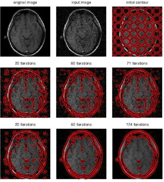
In order to test the effectiveness of our method for the simultaneous restoration and segmentation of noisy images, we compare in Figure 4 the results obtained for the two different cases: without and with restoration. Starting from a noisy image, we show in the middle row the segmentation results (without regularization, i.e., r = 0 and I(k)= I0, ∀k),
and in the bottom row we present the results of joint regularization and segmentation for r = 10. For both cases, the number of iterations in the segmentation step s is set to 10. In the first case, we clearly observe the effect of noise on the evolution of the contours, and this persists until convergence. We also note that in this case, i.e. r = 0, the algorithm compares to the piecewise constant case in the classical Mumford-Shah model presented in [30], which is known to be less effective for noisy images.
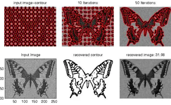
We show in Figure 5 another numerical result of our method using only one level-set function. In the top row, we superpose the evolving curves over the corresponding images I(k), k ∈ {0, 10, 50}. In the bottom row, we show the
final segmentation result (second image) and denoised image (third image) with PS NR = 31.98. For this case, the algorithm converges after 135 iterations.
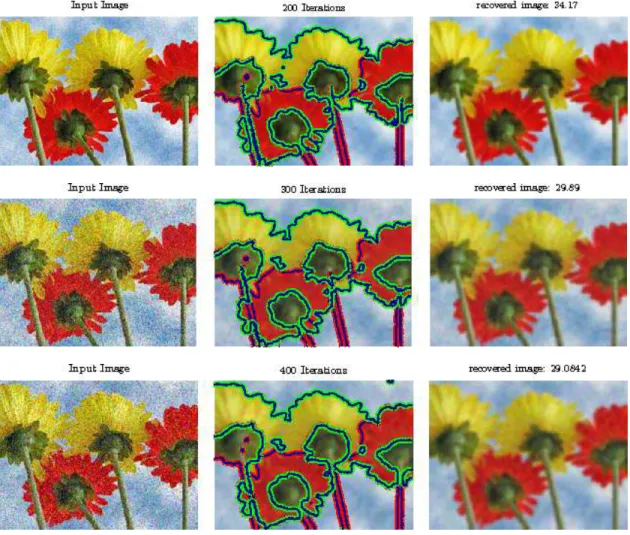
We consider in Figures 6 and 7 the segmentation and restoration of noisy color image. The input image is corrupted with noise as
I0i = Iioriginal+ noise i,
i = r, g, b.
The proposed algorithm is tested in Figures 7 for two types of noise: Gaussian noise and salt-and-pepper noise. In this case, two level-set functions are used (multi-phase), their initialization is shown in Figure 6. The special initialization curves are known to speed up the convergence rate and also to converge to a global minimizer [30]. The obtained results are very satisfactory and confirm the efficiency of the game theory approach to deal with the antagonistic coupling between regularization and segmentation. This can be seen from the quality of the restored images (high PSNR values) as well as from the quality of the contours.
5. Conclusion
The problem of joint image restoration and segmentation rises strong antagonisms between these two objectives. A classical popular method is to use a weighted combination, which poses the problem of parameter tuning (calibration). This problem is known to be tricky and costly, exhibiting numerical stiffness.We have proposed in this paper to formulate the latter problem as a static with complete information game, where restoration uses intensity field to play against segmentation which in turn uses the set of discontinuities. The problem amounts then to find a solution to this game, namely a Nash equilibrium.Then we have presented a relaxation algorithm for computing this equilibrium. It has the advantage that at each step it solves in parallel two classical and “simple” models. The proposed algorithm has been applied to a class of images widely used as benchmarks.
A striking byproduct of our approach is that since only the mean of I is considered in the segmentation step, we have noticed a rapid convergence rate for all the studied images. The numerical experiments demonstrated the efficiency and robustness of our algorithm with respect to parameters and to the noise level.Apart from extending this approach to more complex games, e.g., dynamic with incomplete information, there are many theoretical as well as practical questions that arise thanks to the game approach, among which are the existence of equilibria, the convergence of algorithms of computing them and the sensitivity of solutions to partition strategies between the objectives.
Figure 1: Restoration and segmentation of an image corrupted with Gaussian noise (variance = 0.2) using the proposed algorithm (top row) and using the Mumford-Shah algorithm (bottom row) for ν = 0.02.
Figure 2: Restoration and segmentation of an image corrupted with Gaussian noise (variance = 0.2) using the proposed algorithm (top row) and using the Mumford-Shah algorithm (bottom row) for ν = 0.16.
Figure 3: Restoration and segmentation of an image corrupted with Gaussian noise (variance = 0.2) using the proposed algorithm (top row) and using the Mumford-Shah algorithm (bottom row) for ν = 0.2.
Figure 4: Top row: original, noisy image with Gaussian noise (variance = 0.2) and initial contour. Middle row: restoration and segmentation of image by proposed algorithm with r = 0 (ν = 0.2, µ = 0.01, s = 10). Bottom row: restoration and segmentation of image using the proposed algorithm with r = 10 (ν = 0.2, µ = 0.01, s = 10).
Figure 5: Top row: noisy image with Gaussian noise (variance = 0.2) and initial contour, evolution by iterations. Bottom row: segmentation and restoration of image by the proposed algorithm with (ν = 0.2, µ = 0.01, r = s = 10), for k = 135. CPU time = 117 sec.
Figure 6: Original color image (left) and initial contours for two level-set functions (right).
Figure 7: Segmentation and restoration of noisy color image and PSNR values. First column: noisy image with Gaussian noise, variance = 0.02 (top) and variance = 0.1 (middle). Noisy image with salt-and-pepper noise with noise density d = 0.2 (bottom). Second and third columns: the corresponding segmented and restored image by the proposed algorithm with (ν = 0.2, µ = 0.01, r = s = 10). CPU time = 588 sec, 907 sec and 1203 sec, respectively.
References
[1] R. Aboulaich, A. Habbal, and N. Moussaid. Optimisation multicrit`ere - une approche par partage des variables. Revue Africaine en
Informa-tique et Math´emaInforma-tiques Appliqu´ees (ARIMA), 13:77–89, 2010.
[2] L. Ambrosio. Existence theory for a new class of variational problems. Archive for Rational Mechanics and Analysis, 111:291–322, 1990. [3] L. Ambrosio and V.M. Tortorelli. Approximation of functionals depending on jumps by elliptic functionals via γ-convergence. Commun.
Pure Appl. Math., 43(8):999–1036, 1990.
[4] G. Aubert and P. Kornprobst. Mathematical Problems in Image Processing: Partial Differential Equations and the Calculus of Variations, volume 147 of Applied Mathematical Sciences. Springer-Verlag, New York, 2nd edition, 2006.
[5] Tamer Bas¸ar. Relaxation techniques and asynchronous algorithms for on-line computation of noncooperative equilibria. J. Econom. Dynam.
Control, 11(4):531–549, 1987.
[6] B. Bourdin. Image segmentation with a finite element method. M2AN Math. Model. Numer. Anal., 33(2):229–244, 1999.
[7] B. Bourdin and A. Chambolle. Implementationof a finite elements approximation of the mumford-shah functional. Numer. Math., 85(4):609– 646, 2000.
[8] V. Caselles, R. Kimmel, and G. Sapiro. Geodesic active contours. International Journal of Computer Vision, 22:61–79, 1997.
[9] A. Chambolle. Image segmentation by variational methods: Mumford and shah functional and the discrete approximation. SIAM Journal of
applied Mathematics, 55(3):827–863, 1995.
[10] A. Chambolle, V. Caselles, D. Cremers, M. Novaga, and T. Pock. An introduction to total variation for image analysis. In M. Fornasier, editor, Theoretical Foundations and Numerical Methods for Sparse Recovery, volume 9 of Radon Series on Computational and Applied
Mathematics, pages 263–340. De Gruyter, Berlin, New York, 2010.
[11] A. Chambolle and G. Dal Maso. Discrete approximation of the mumford-shah functional in dimension two. M2AN Math. Model. Numer.
Anal., 33(4):651–672, 1999.
[12] T. F. Chan and J. Shen. Image Processing and Analysis: variational, PDE, wavelet, and stochastic methods. SIAM, Philadelphia, 2005. [13] L. C. Evans and R. F. Gariepy. Measure Theory and Fine Properties of Functions. Studies in Advanced Mathematics. CRC Press, Florida,
1992.
[14] R. Gibbons. Game Theory for Applied Economists. Princeton University Press, Princeton, NJ, 1992.
[15] M. Gobbino. Finite difference approximation of the mumford-shah functional. Commun. Pure Appl. Math., 51(2):197–228, 1998. [16] A. Habbal. A topology Nash game for tumoral antiangiogenesis. Structural and Multidisciplinary Optimization, 30(5):404–412, 2005. [17] A. Habbal, J. Petersson, and M. Thellner. Multidisciplinary topology optimization solved as a Nash game. Int. J. Numer. Meth. Engng,
61:949–963, 2004.
[18] Z. Hongmei and W. Mingxi. Improved Mumford-Shah functional for coupled edge-preserving regularization and image segmentation.
EURASIP Journal on Applied Signal Processing, pages 1–9, 2006.
[19] M. Kass, A. Witkin, and D. Terzopoulos. Snakes: Active contour models. International Journal of Computer vision, 1:321–331, 1988. [20] Shu Li and Tamer Bas¸ar. Distributed algorithms for the computation of noncooperative equilibria. Automatica J. IFAC, 23(4):523–533, 1987. [21] R. Malladi, J. A. Sethian, and B. C. Vemuri. Shape modeling with front propagation: A level set approach. IEEE Transactions on Pattern
Analysis and Machine Intelligence, 17(2):158–175, 1995.
[22] D. Mumford and J. Shah. Optimal approximations by piecewise smooth functions and variational problems. Commun. Pure Appl. Math., 42(5):577–685, 1989.
[23] S. Osher and J. A. Sethian. Fronts propagating with curvature-dependent speed: Algorithms based on Hamilton-Jacobi formulations. Journal
of Computational Physics, 79(1):12–49, 1988.
[24] P. Perona and J. Malik. Scale-space and edge detection using anisotropic diffusion. IEEE Trans. Pattern Analysis and Machine Intelligence, 12:629–639, 1990.
[25] T. Pock, D. Cremers, H. Bischof, and A. Chambolle. An algorithm for minimizing the Mumford-Shah functional. In 12th IEEE International
Conference on Computer Vision, 2009.
[26] L. I. Rudin, S. Osher, and E. Fatemi. Nonlinear total variation based noise removal algorithms. Physica D, 60:259–268, 1992. [27] G. Sapiro. Geometric Partial Differential Equations and Image Analysis. Cambridge University Press, 2001.
[28] 0. Scherzer, M. Grasmair, H. Grossauer, M. Haltmeier, and F. Lenzen. Variational Methods in Imaging, volume 167 of Applied Mathematical
Sciences. Springer, New York, 2009.
[29] S. Uryas’ev and R. Y. Rubinstein. On relaxation algorithms in computation of noncooperative equilibria. IEEE Transactions on Automatic
Control, 39(6):1263–1267, 1994.
[30] L. A. Vese and T. F. Chan. A multiphase level set framework for image segmentation using the Mumford and Shah model. International
Journal of Computer Vision, 50:271–293, 2002.
[31] Y. Zhang. Fast segmentation for the piecewise smooth Mumford-Shah functional. International Journal of Signal Processing, 2:245–250, 2006.