Inventory Investment Dynamics and Recoveries: A Comparison of Manufacturing and Retail Trade Sectors

HAL Id: hal-01515613

https://hal.archives-ouvertes.fr/hal-01515613

HAL is a multi-disciplinary open access

archive for the deposit and dissemination of sci-entific research documents, whether they are pub-lished or not. The documents may come from teaching and research institutions in France or abroad, or from public or private research centers.

L’archive ouverte pluridisciplinaire HAL, est destinée au dépôt et à la diffusion de documents scientifiques de niveau recherche, publiés ou non, émanant des établissements d’enseignement et de recherche français ou étrangers, des laboratoires publics ou privés.

Inventory Investment Dynamics and Recoveries: A

Comparison of Manufacturing and Retail Trade Sectors

Frédérique Bec, Marie Bessec

To cite this version:

Frédérique Bec, Marie Bessec. Inventory Investment Dynamics and Recoveries: A Comparison of Manufacturing and Retail Trade Sectors. Economics Bulletin, Economics Bulletin, 2013, 33 (3). �hal-01515613�

DOCUMENT

DE TRAVAIL

N° 400

INVENTORY INVESTMENT DYNAMICS AND RECOVERIES:

A COMPARISON OF MANUFACTURING

AND RETAIL TRADE SECTORS

Frédérique BEC and Marie BESSEC

DIRECTION GÉNÉRALE DES ÉTUDES ET DES RELATIONS INTERNATIONALES

INVENTORY INVESTMENT DYNAMICS AND RECOVERIES:

A COMPARISON OF MANUFACTURING

AND RETAIL TRADE SECTORS

Frédérique BEC and Marie BESSEC

October 2012

Les Documents de travail reflètent les idées personnelles de leurs auteurs et n'expriment pas nécessairement la position de la Banque de France. Ce document est disponible sur le site internet de la Banque de France « www.banque-france.fr ».

Working Papers reflect the opinions of the authors and do not necessarily express the views of the Banque de France. This document is available on the Banque de France Website “www.banque-france.fr”.

Inventory Investment Dynamics and Recoveries: A

Comparison of Manufacturing and Retail Trade

Sectors

Fr´

ed´

erique Bec

Marie Bessec

1

THEMA, Universit´e de Cergy-Pontoise, CREST-INSEE, Banque de France. email: bec@ensae.fr

2

Banque de France, DGEI-DCPM-DIACONJ, Paris, France et LEDa-Universit´e Paris Dauphine. We thank Lars Wenzel and the participants of the CIRET conference in Vienna, Sophie Haincourt, Bertrand Pluyaud and Pierre Sicsic for their comments and suggestions. This paper reflects the opinions of the authors and does not necessarily express the views of the Banque de France.

R´esum´e : Cet article examine l’existence d’effets de rebond dans la variation des stocks en sortie de r´ecession `a partir des donn´ees d’enquˆete de la Commission europ´eenne. Nous utilisons les soldes d’opinions relatifs aux stocks dans l’industrie manufacturi`ere et le commerce de d´etail pour la France, l’Allemagne et la zone euro. Nos r´esultats confirment l’existence d’un effet de rebond dans le comportement de stockage des entreprises, au cours des trimestres qui ont suivi les r´ecessions. Ce r´esultat pourrait `a son tour expliquer le rebond du taux de croissance du PIB r´eel mis en ´evidence dans les ´etudes empiriques ant´erieures. Par ailleurs, selon nos estimations, l’effet de rebond des stocks se produit plus tard et dure plus longtemps dans l’industrie manufacturi`ere que dans le commerce de d´etail.

Mots-cl´es : Mod`ele `a seuil, effet de rebond, cycle des affaires, stocks.

Code JEL : C22, E32.

Abstract: This paper explores the existence of a bounce-back effect in inventory

in-vestment using the European Commission opinion survey on stocks of finished products in manufacturing and retail trade sectors. The data are quarterly balance for France, Germany and a European aggregate, from 1985q1 to 2011q4. Our empirical findings support the existence of a high recovery episode for inventory investment, during the quarters immediately following the recessions. This could in turn explain the real GDP growth rate bounce-back pointed out in previous empirical studies. Moreover, according to our estimates, the inventory investment bounce-back occurs later and lasts longer in manufacturing than in retail trade sector.

Keywords: Threshold auto-regression, bounce-back effects, business cycles, inventory

investment.

Introduction

Since Abramovitz [1950], the role of inventory investment in business cycles is consid-ered as important, even though often neglected. This belief basically stems from the stylized facts that inventory investment is procyclical and in general slightly positively correlated with sales, while the variance of production is greater than the variance of sales.3 _{Hence, as production is the sum of final sales and inventory investment from a} national accounting perspective, the latter is suspected to exacerbate business cycles.

Yet, a growing number of empirical studies find evidence of a high-growth recovery phase following contractions in real GDP growth rate data (see e.g. Sichel [1994], Kim, Morley and Piger [2005], Bec, Bouabdallah and Ferrara [2011a] or Bec, Bouabdallah and Ferrara [2011b], Morley and Piger [2012]). To our knowledge, the origins of this bounce-back phenomenon have hardly been explored so far. The theoretical literature on inventory investment basically considers four motives for holding inventories. The production smoothing motive — see e.g. Blinder [1986] for a comprehensive presentation — was the most popular one until the eighties. Probably due to its counter-factual prediction regarding the relative volatility of output and final sales, alternative motives have been put forward since then: i) the reduction of fixed order costs which grounds the so-called (S, s) rule was first promoted by Blinder [1981], ii) the avoidance of stockouts is the motive proposed by Kahn [1987] while iii) the production-costs smoothing motive is analyzed in a partial equilibrium model by Eichenbaum [1989]. Nevertheless, even though a motive may bunch production by producing more than sales at the firm level — for instance to smooth a transitory favorable cost shock or when the floor of minimum stocks, s, is reached — its impact on aggregate output is not trivial. Within a dynamic stochastic general equilibrium setup, recent works by Wang and Wen [2009] and Wang, Wen and Xu [2011] suggest that the production-cost smoothing motive or a firm-level (S, s) policy for holding inventories respectively may explain a bounce-back effect in the aggregate output as long as there is one in the inventory investment. This motivates the

3

See Blinder and Maccini [1991] for a detailed discussion of these stylized facts and the competing economic theories as of the end of the eighties.

empirical investigation of inventory investment dynamics proposed in this paper. Indirect empirical evidence for the inventory investment bounce-back effect is pro-vided in Sichel [1994] from US data. Basically, since the real output is the sum of the final sales and the inventory investment, this author tests for a bounce-back effect in final sales using a very simple regression allowing the average growth rate of the final sales to switch across expansion/contraction/recovery phases over the business cycle. As the lack of bounce-back effect null hypothesis is not rejected for the final sales, whereas it is for the real GDP growth rate, Sichel [1994] concludes that the latter originates in the inventories bounce-back. More recently, Bec and Ben Salem [2012] have used French national account data to test for the presence of a bounce-back effect in in-ventory investment contribution to real GDP growth rate. More precisely, they retain the bounce-back augmented threshold autoregressive model proposed recently by Bec et al. [2011b] to account for periods of high-growth recoveries following the cycle trough4_. Their first results are quite encouraging, but still open to criticism due to the very nature of the data. Actually, inventory investment data are measured by the French national statistics Institute (INSEE) as the difference between the national sources and uses other than inventories, namely intermediate consumption, final consumption, gross fixed cap-ital formation and exports. If the latter were perfectly measured, then so would the inventory investment data. In general, any measurement error in the various uses will contaminate the measure of inventory investment. As a consequence, these inventory investment data are also subject to large revisions.

Our contribution to this literature is twofold. First, we circumvent this data issue by using European opinion survey data instead. Survey data gives a qualitative but direct assessment by the firm leaders on the level of inventories and is not subject to revision (but for the last available observation so as to include the latest answers). Second, the use of survey data gives us the opportunity to distinguish the inventory investment in finished goods by industrial firms and the one by retail traders5_{. This is not possible}

4

See Kim et al. [2005] or Morley and Piger [2012] for an extension of the Markov-Switching model which allows bounce-back effects.

5

PMI survey also contains questions about the stocks of purchases and the stocks of finished goods in manufacturing industry and retail trade.

with the quarterly accounts where only a decomposition by products is available. This is interesting since the inventory behavior is likely to depend on the position of the firm in the production process, as emphasized in e.g. Blinder and Maccini [1991] and de Rougemont [2011]. For instance, inventories of finished goods are expected to adjust quicker to the desired level in retail trade than in manufacturing. Inventory investment is also found to be less volatile in the latter sector than in the former, according to Blinder and Maccini [1991]. Besides French data, we also analyze German and aggregate European data for the period 1985Q1-2011Q4.

Our results suggest that both the linearity hypothesis and the null of no bounce-back in the threshold model are strongly rejected in the three cases. Moreover, the introduc-tion of the bounce-back effect in the threshold model clearly improves the short-term forecasting performance for Germany and the European aggregate in the manufactur-ing sector and for France and the European aggregate in the retail trade sector. These results are compatible with the view that the real GDP growth rate bounce-back may originate in the inventory investment behavior. As regards the comparison of inventory investment behavior across sectors, it turns out that the bounce-back occurs later and lasts longer in manufacturing than in retail trade sector.

The paper is organized as follows. Section 1 briefly presents the bounce-back aug-mented threshold autoregressive model and discusses the various shapes of bounce-back functions as special cases of the general model. Section 2 describes the data and presents the linearity tests before reporting the estimation results. Section 3 evaluates the short-run forecasting performances of the bounce-back models, paying careful attention to the last recession episode. Section 4 concludes.

1

The bounce-back augmented threshold

autoregres-sive model

The model considered throughout this paper was first introduced by Bec et al. [2011b]. Denoting by ztthe inventory investment series that we will discuss more precisely in the

next section, the bounce-back augmented threshold autoregression is the following: φ(L)zt = µt+ et, (1) with µt defined by µt = γ0(1 − st) + γ1st +λ1st ℓ+m X j=ℓ+1 s_t−j+ λ2(1 − st) ℓ+m_X j=ℓ+1 s_t−j+ λ3 ℓ+m X j=ℓ+1 ∆y_t−j−1s_t−j, (2) and where φ(L) is a lag polynomial of order p with roots lying outside the unit circle

and et i.i.d. N (0,σ). In the second equation, ℓ and m are non-negative integers and

correspond respectively to the delay with which the bounce-back effect occurs and to its duration. The λi’s parameters measure the size of the bounce-back effect. The variable st denotes the transition function which takes on the value zero or one. In our model, st is defined as:

st= 0 if ∆yt−1> κ and 1 otherwise, (3)

where κ is a real-valued threshold parameter and ∆y_t−1 is the lagged growth rate of

real GDP. The model given by equations (1) to (3) allows for an asymmetric behavior across regimes. Here, st = 1 is identified as the low, or contraction regime by assuming κ < 0. It implies that the intercept in equation (1) is γ0 if the lagged growth rate of real GDP, ∆y_t−1, is larger than the threshold κ (i.e. high, or expansion regime) and γ1 otherwise. The remainder of equation (2) defines a very flexible form for the bounce-back phenomenon. If λ1 is positive, then the term λ1st

Pℓ+m

j=ℓ+1st−j will increase µt above its low regime value (γ1), ℓ + 1 quarters after the beginning of the recession and so until the recession comes to its end. Hence, this term activates during the recession only. If λ2 is positive, then the value of µt will exceed γ0 immediately after the recession is over. Finally, note that the third term of the bounce-back function depends on the depth of the last recession through the variable ∆y_t−j−1: negative values of λ3 will drive µt above (γ0(1 − st) + γ1st) proportionally to the depth of the recession.

The µtfunction defined by equation (2) has the nice property that it nests the three models first proposed by Kim et al. [2005], namely the U-, V- and Depth-shaped

back6 _{as well as the no bounce-back — standard threshold — model with the following} linear restrictions:

- HN

0 : λi = 0 ∀i corresponds to the standard (no bounce-back) threshold model,

- HU

0: λ1 = λ2 = λ 6= 0 and λ3 = 0 gives the U-shaped model, hereafter denoted BBU, - HV

0: λ2 6= 0 and λ1 = λ3 = 0 gives the BBV model, - HD

0: λ3 6= 0 and λ1 = λ2 = 0 defines the BBD model.

The null hypothesis of linearity amounts here to test the joint hypothesis λ1 = λ2 = λ3 =

0 and γ0 = γ1, i.e. µt becomes a constant term. Obviously, the threshold parameter

is unidentified under this null. Consequently, the linearity test will rely on a SupLR statistics along the lines proposed by Davies [1987] and its bootstrapped p-value will be computed following Hansen [1996]. By contrast, since there are nuisance parameter free,

the four assumptions HN

0 , HU0, HV0 and HD0 can be tested from a LR statistics which has a standard Chi-squared distribution.

Finally, the general model defined here by equations (1) to (3) will be denoted BBF(p, m, ℓ), as in Bec et al. [2011b]. This BBF model is estimated along the lines described in Bec et al. [2011b], from the nonlinear least squares method using a triple grid search on the ℓ, m and κ parameters, for ℓ ∈ {0, 1, 2}, m ∈ {0, . . . , 8} and κ ∈ [κl; κu] where κl is the 5%-quantile of the switching variable ∆yt and κu = 0 so as to define the low regime as a recession regime.

2

Inventories investment nonlinear dynamics

The data we consider throughout the analysis come from the European Commission total manufacturing industry and retail trade opinion survey, regarding the assessment of stocks. For industry it corresponds to Question 4 of the business opinion survey, namely:

“Do you consider your current stock of finished products to be...?

6

• + too large (above normal)

• = adequate (normal for the season) • - too small (below normal)”

while for retail trade, it corresponds to Question 2 of the retail trade survey, namely: “Do you consider the volume of stock you currently hold to be...?”, with the same three items as potential replies. The indicators are expressed as the seasonally adjusted balance (in percentage points) of positive over negative results.

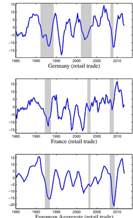
The data are available at the monthly frequency, but since the GDP are quarterly data, the survey balances are converted into quarterly frequency by averaging monthly observations. Our sample includes data for France, Germany and Europe over the period 1985Q1 to 2011Q4 but for the retail trade survey for Europe which starts in 1985Q4 only. To make these survey data comparable to inventory investment, we take their first difference. Actually, the questions clearly focus on the volume of inventories in levels. Hence, the use of series in first difference is more relevant since a lower destocking captured by a decrease in the survey variable from a high level contributes positively to the GDP growth rate and thus can take part to the rebound in real GDP growth. Then, we use this series with inverted sign because a positive survey balance is most likely to correspond to a decrease in inventory investment. Indeed a positive balance means that a majority of business leaders consider their stock as too large, which implies at least that they stop increasing it further. The two countries and the European aggregate data are plotted in Figure 1, see Appendix.

Table 1 below reports parameters m, ℓ and κ estimates once the lag length parameter p is fixed at the smallest value which eliminates estimated residuals serial correlation7. The columns SupLR and p−value report the results of the SupLR linearity test for 2,000 random draws under the null. As can be seen from the bootstrapped p−values of the tests reported in the last column of Table 1, the linearity null hypothesis is strongly rejected for the inventory investment in the total manufacturing industry. The evidence

7

Regarding the retail trade sector data, even though the BBF model residuals were found not serially correlated with zero lag in the German and French cases, it turns out that the third lag provides significant information regarding the dynamics of ∆xtand hence, it is kept for the subsequent analysis.

Table 1: Linearity tests results: Model I

Country p mˆ ℓˆ ˆκ SupLR p-value Manufacturing DE 1 4 1 -0.02 37.84 0.00 FR 1 3 2 -0.11 15.41 0.01 EA 1 4 1 -0.07 33.43 0.00 Retail trade DE 3 2 0 -0.18 13.50 0.08 FR 3 2 0 -0.11 9.75 0.09 EA 2 2 0 -0.23 11.12 0.15

of nonlinearity is only slightly weaker in the retail trade sector. Regarding the bounce-back duration, it is longer for manufacturing (three to four quarters) than for retail trade (two quarters). It is also worth noticing that the effect activates earlier in the retail trade sector than in the manufacturing industry where it is delayed by one or two quarters. These findings are well in line with the widespread view that the adjustment of inventories to the desired level is quicker in retail trade than in manufacturing. As stressed by Blinder and Maccini [1991] from U.S. data, manufacturers’ inventories of finished goods are the least volatile component of inventory investment.

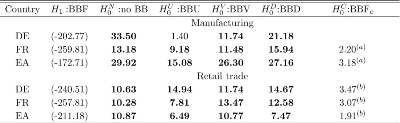
Let us now test for the existence and more specific shapes of the bounce-back effect in Equation (2). The log-likelihood ratio test statistics corresponding to the various hypothesis are reported in Table 2 below. Regarding the manufacturing sector, the null of no bounce-back effect is always strongly rejected. In the German case, the U-shaped bounce-back model is not rejected since the p−value of the χ2_{(2) distributed LR} statistics is 50%. In France and Europe, the standard U-, V-, and Depth-shaped bounce-back functions are strongly rejected. A closer look at the BBF model estimates8 _reveals that λ3 is not significantly different from zero, which is confirmed by the LR statistics reported in the last column of Table 2. This constrained BBF model will hence be kept for the subsequent analysis. In the retail trade sector, the null of no bounce-back is again strongly rejected. So are the existing U, V and D-shaped bounce-back patterns. When

8

Table 2: LR-Test for the shape of the bounce-back function

Country H1:BBF H0N :no BB H0U :BBU H0V:BBV H0D:BBD H0C:BBFc

Manufacturing DE (-202.77) 33.50 _1.40 11.74 21.18 FR (-259.81) 13.18 9.18 11.48 15.94 _2.20(a) EA (-172.71) 29.92 15.08 26.30 27.16 _3.18(a) Retail trade DE (-240.51) 10.63 14.94 11.74 14.67 _3.47(b) FR (-257.81) 10.28 7.81 13.47 12.58 _3.07(b) EA (-211.18) 10.87 6.49 10.77 7.47 _1.91(b)

Notes: Figures into parenthesis are log-likelihoods.

Bold characters denote rejection of the null at the 5%-level.

Superscripts (a) and (b) correspond to the constraints λ3= 0 and λ2= λ3 = 0 respectively.

looking at the BBF model estimates9_{, it turns out that only λ}

1 is significantly different

from zero. The test of the joint hypothesis λ2 = λ3 = 0 — reported in the last column

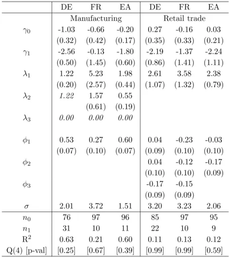
of Table 2 — never rejects the null. Finally, in Table 3 below, we report the constrained

BBF versions but for German manufacturing data where the BBU model is retained. λ1

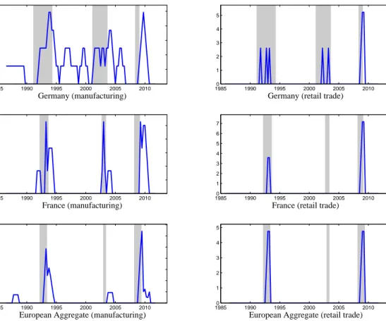
and λ2’ estimates have the expected sign in the six models, i.e. they are positive which corresponds to a larger value for µt. A quick glance at the estimated bounce-back effects, i.e. ˆµt− ˆγ0(1 − st) − ˆγ1st, see Figure 2 reported in appendix, reveals that it activates more often and lasts longer in the manufacturing sector (graphs on the left-hand side) than in the retail trade (right-hand side). The bounce-back magnitude is comparable in both sectors during the last recession, but it is triggered earlier in the recession in the retail trade sector than in manufacturing. Since λ2 = λ3 = 0 for retail trade data, the bounce-back effect stops as soon as the recession is over. During the 1992 and 2002 recessions, the estimated bounce-back effects are twice as large in the manufacturing sector as in the retail trade sector. In the later, the recession which occurred in the early 2000s did not generate any bounce-back effect according to French and European models estimates.

9

Not reported but available upon request.

Table 3: Models estimates

DE FR EA DE FR EA

Manufacturing Retail trade γ0 -1.03 -0.66 -0.20 0.27 -0.16 0.03 (0.32) (0.42) (0.17) (0.35) (0.33) (0.21) γ1 -2.56 -0.13 -1.80 -2.19 -1.37 -2.24 (0.50) (1.45) (0.60) (0.86) (1.41) (1.11) λ1 1.22 5.23 1.98 2.61 3.58 2.38 (0.20) (2.57) (0.44) (1.07) (1.32) (0.79) λ2 1.22 1.57 0.55 (0.61) (0.19) λ₃ 0.00 0.00 0.00 φ1 0.53 0.27 0.60 0.04 -0.23 -0.03 (0.07) (0.10) (0.07) (0.09) (0.10) (0.10) φ2 0.04 -0.12 -0.17 (0.10) (0.10) (0.09) φ3 -0.17 -0.15 (0.09) (0.09) σ 2.01 3.72 1.51 3.20 3.23 2.06 n0 76 97 96 85 97 95 n1 31 10 11 22 10 9 R2 _{0.63 0.21 0.60 0.11 0.13 0.12} Q(4) [p-val] [0.25] [0.67] [0.39] [0.99] [0.99] [0.59] Notes: Figures into parenthesis are standard deviations. Characters in italic denote constrained values.

ni is the number of obs. in regime i.

3

Forecasting accuracy evaluation

As an additional check of the added value of the BBF models over the linear specifica-tion, the one-step ahead forecasts are calculated from a pseudo-real time analysis using recursive regressions.

Given that our final observation date, Tf, is 2011Q4, we begin the forecast perfor-mance evaluation from T0=2006Q1. Then, for all t ∈ {T0, ..., Tf − 1}, we estimate the model from the first available observation until t, and use this estimate to compute the

one-step-ahead forecasts. Then, we decompose the last crisis episode into the recession time and the recovery, beginning the quarter just after the trough. The recession dates come from the ECRI for Germany and France and were calculated following the Bry and Boschan [1971] algorithm adapted to quarterly data for the European aggregate. So as to assess the added value of the nonlinear features of the model, these forecasts are compared with those from a benchmark linear autoregression, i.e. imposing a

con-stant value for µt in equation (1). The added value of the bounce-back term is also

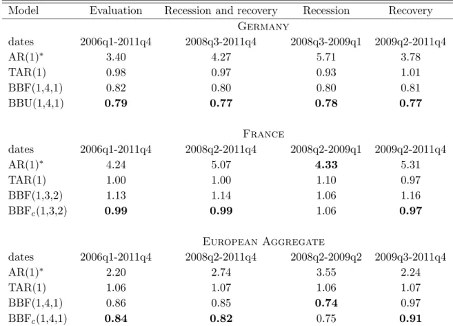
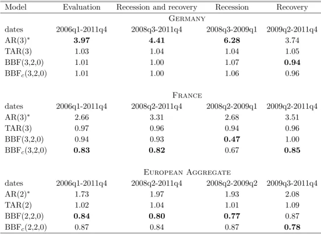
assessed by comparing these forecasts to a standard SETAR model, i.e. setting all the λi’s to zero, i = 1, 2, 3, in equation (2). Finally, we focus on point forecasts accuracy as measured by the Root Mean Squared Error (RMSE) criteria. For the manufacturing (respectively retail trade) sector, they are reported in Table 4 (resp. 5). A quick glance at the RMSEs obtained for the manufacturing sector reveals that it is almost always the case that the BBF models forecasts outperform the ones from the linear (AR) or the standard threshold (TAR) autoregressions. For the evaluation sample, the ratio of the BBF and AR models RMSEs is 0.79 in Germany and 0.84 in Europe. By contrast, the gain in forecasting accuracy is rather disappointing for the French case: here, the best ratio is obtained during the last recovery but it reaches only 0.97. The results obtained for the retail trade sector are more contrasted in terms of forecast accuracy. Actually, they are quite disappointing in the German case where the only sub-period favorable to the bounce-back model is the last two years after the end of the recession. For the evaluation sample and the 2008q3-2011q4 sub-sample, the BBF models, whether con-strained or not, perform exactly as well as the linear model. By contrast, French results in the retail trade are strongly favorable to the BBF model where the gain typically lies between 15 to 30%, and reaches as much as 53% for the unconstrained BBF model during the last recession. For the European data, the results obtained in the retail trade sector are comparable to those obtained in the manufacturing sector, except that here, the unconstrained BBF model outperforms its constrained version in all sub-samples but the last recovery.

Table 4: 1-step ahead forecasts (relative RMSE criterion): Manufacturing

Model Evaluation Recession and recovery Recession Recovery Germany dates 2006q1-2011q4 2008q3-2011q4 2008q3-2009q1 2009q2-2011q4 AR(1)∗ _{3.40 4.27 5.71 3.78} TAR(1) 0.98 0.97 0.93 1.01 BBF(1,4,1) 0.82 0.80 0.80 0.81 BBU(1,4,1) 0.79 0.77 0.78 0.77 France dates 2006q1-2011q4 2008q2-2011q4 2008q2-2009q1 2009q2-2011q4 AR(1)∗ _{4.24 5.07} 4.33 _5.31 TAR(1) 1.00 1.00 1.10 0.97 BBF(1,3,2) 1.13 1.14 1.06 1.16 BBFc(1,3,2) 0.99 0.99 1.06 0.97 European Aggregate dates 2006q1-2011q4 2008q2-2011q4 2008q2-2009q2 2009q3-2011q4 AR(1)∗ _{2.20 2.74 3.55 2.24} TAR(1) 1.06 1.07 1.06 1.07 BBF(1,4,1) 0.86 0.85 0.74 _0.97 BBFc(1,4,1) 0.84 0.82 0.75 0.91

∗_{: All RMSE, but the ones of the AR models, are given relative to the AR model RMSE.}

4

Conclusion

This paper explores the existence of a bounce-back effect in inventory investment using the European Commission opinion survey on stocks of finished products in manufactur-ing and retail trade. The data are quarterly balance (in percentage points) of positive over negative results for France, Germany and a European aggregate, from 1985q1 to 2011q4. Using the bounce-back augmented threshold autoregression first proposed by Bec et al. [2011a], our empirical findings support the existence of a high recovery episode for inventory investment, during the quarters immediately following the recessions. As expected, this bounce-back episode occurs later and lasts longer in manufacturing than in retail trade sector. On the whole, the inventory investment bounce-back found here

Table 5: 1-step ahead forecasts (relative RMSE criterion): Retail trade

Model Evaluation Recession and recovery Recession Recovery Germany dates 2006q1-2011q4 2008q3-2011q4 2008q3-2009q1 2009q2-2011q4 AR(3)∗ 3.97 4.41 6.28 _3.74 TAR(3) 1.03 1.04 1.04 1.05 BBF(3,2,0) 1.01 1.00 1.07 0.94 BBFc(3,2,0) 1.01 1.00 1.06 0.96 France dates 2006q1-2011q4 2008q2-2011q4 2008q2-2009q1 2009q2-2011q4 AR(3)∗ _{2.66 3.31 2.68 3.51} TAR(3) 0.97 0.96 0.94 0.96 BBF(3,2,0) 0.94 0.93 0.47 _1.00 BBFc(3,2,0) 0.83 0.82 0.67 0.85 European Aggregate dates 2006q1-2011q4 2008q2-2011q4 2008q2-2009q2 2009q3-2011q4 AR(2)∗ _{1.73 1.97 1.93 2.08} TAR(2) 1.02 1.04 1.01 1.09 BBF(2,2,0) 0.84 0.80 0.77 _0.87 BBFc(2,2,0) 0.87 0.84 0.87 0.78

∗_{: All RMSE, but the ones of the AR models, are given relative to the AR model RMSE.}

could explain the real GDP growth rate bounce-back pointed out in previous empirical studies. In order to check this, the extension of the analysis to the joint dynamics of real GDP growth rate and inventory investment opinion survey data is on our research agenda.

References

Abramovitz, M., Inventories and Business Cycles, New York: National Bureau of Eco-nomic Research, 1950.

Bec, F. and M. Ben Salem, Inventory Investment and the Business Cycle: The Usual Suspect, Working Paper 2012-tba, CREST, Paris 2012.

, O. Bouabdallah, and L. Ferrara, The possible shapes of recoveries in Markov switching models, Working Paper 2011-02, CREST 2011a.

, , and , The European Way Out of Recessions, Manuscript 2011b.

Blinder, A.S., Retail Inventory Behavior and Business Fluctuations, Brookings Papers on Economic Activity, 1981, 2, 443–505.

, Can the Production Smoothing Model of Inventory Behavior Be Saved, Quarterly Journal of Economics, 1986, 101 (3), 431–453.

and L.J. Maccini, Taking Stock: A Critical Assessment of Recent Research on Inventories, Journal of Economic Perspectives, 1991, 5 (1), 73–96.

Bry, G. and C. Boschan, Cyclical Analysis of Time Series: Selected Procedures and Computer Programs, New York and London: Columbia University Press, 1971. Davies, R. B., Hypothesis Testing When a Nuisance Parameter is Present Only Under

the Alternative, Biometrika, 1987, 74, 33–43.

de Rougemont, P., Les stocks dans la crise, Bulletin de la Banque de France, 2011, 183, 27–46.

Eichenbaum, M., Some Empirical Evidence on the Production Level and Production Cost Smoothing Models of Inventories, American Economic Review, 1989, 79 (4), 853–864.

Hansen, B.E., Inference when a Nuisance Parameter Is Not Identified Under the Null Hypothesis, Econometrica, 1996, 64 (2), 413–430.

Kahn, J., Inventories and the Volatility of Production, The American Economic Review, 1987, 77 (4), 667–679.

Kim, C.-J., J. Morley, and J. Piger, Nonlinearity and the permanent effects of recessions, Journal of Applied Econometrics, 2005, 20, 291–309.

Morley, J. and J. Piger, The asymmetric business cycle, Review of Economics and Statistics, 2012, 94, 208–221.

Sichel, E., Inventories and the Three Phases of the Business Cycles, Journal of Business and Economic Statistics, 1994, 12 (3), 269–277.

Wang, P. and Y. Wen, Inventory Accelerator in General Equilibrium, Working Paper 010, Federal Reserve Bank of St. Louis 2009.

, , and Z. Xu, When Do Inventories Destabilize the Economy? An Analytical

Approach to (S,s) Policies, Working Paper 014, Federal Reserve Bank of St. Louis 2011.

APPENDIX

Germany (retail trade)

1985 1990 1995 2000 2005 2010 −15 −10 −5 0 5 10 15 France (manufacturing) 1985 1990 1995 2000 2005 2010 −20 −15 −10 −5 0 5 10 15

France (retail trade)

1985 1990 1995 2000 2005 2010 −15 −10 −5 0 5 10 15

European Aggregate (manufacturing)

1985 1990 1995 2000 2005 2010 −15 −10 −5 0 5 10

European Aggregate (retail trade)

1985 1990 1995 2000 2005 2010 −20 −15 −10 −5 0 5 10 15

Germany (manufacturing) 19850 1990 1995 2000 2005 2010 1 2 3 4 5

Germany (retail trade)

19850 1990 1995 2000 2005 2010 1 2 3 4 5 France (manufacturing) 19850 1990 1995 2000 2005 2010 1 2 3 4 5

France (retail trade)

19850 1990 1995 2000 2005 2010 1 2 3 4 5 6 7

European Aggregate (manufacturing)

19850 1990 1995 2000 2005 2010 1 2 3 4 5 6 7

European Aggregate (retail trade)

19850 1990 1995 2000 2005 2010 1 2 3 4 5

Figure 2: Estimated bounce-back functions

Documents de Travail

385. G. Dufrénot and K. Triki, “Public debt ratio and its determinants in France since 1890 – Does econometrics supports the historical evidence? ,” July 2012

386. G. Dufrénot and K. Triki, “Why have governments succeeded in reducing French public debt historically and can these successes inspired us for the future? An historical perspective since 1890,” July 2012

387. G. Gaballo, “Private Uncertainty and Multiplicity,” July 2012

388. P. Towbin, “Financial Integration and External Sustainability,” July 2012

389. G. Cette, N. Dromel, R. Lecat and A.-C. Paret, “Labour relations quality and productivity: An empirical analysis on French firms,” July 2012

390. D. Beau, L. Clerc and B. Mojon, “Macro-Prudential Policy and the Conduct of Monetary Policy,” July 2012 391. E. Challe, B. Mojon and X. Ragot, “Equilibrium Risk Shifting and Interest Rate in an Opaque Financial

System,” July 2012

392. D. Fuentes Castro, “Funding for green growth,” August 2012

393. A. Cheptea, L. Fontagné and S. Zignago, “European Export Performance,” August 2012

394. J-S. Mésonnier and D. Stevanovic, “Bank leverage shocks and the macroeconomy: a new look in a data-rich environment,” August 2012

395. J-P. Renne, “A model of the euro-area yield curve with discrete policy rates,” September 2012 396. M. Bussiere and A. Ristiniemi, “Credit Ratings and Debt Crises,” September 2012

397. A. Monfort and F. Pegoraro, “Asset Pricing with Second-Order Esscher Transforms,” September 2012 398. S. Gabrieli, “Too-connected versus too-big-to-fail: banks’ network centrality and overnight interest rate,”

September 2012

399. Y. Kalantzis, R. Kambayashi and S. Lechevalier, “Wage and Productivity differentials in Japan. The Role of Labor Market Mechanisms,” September 2012

400. F. Bec and M. Bessec, “Inventory Investment Dynamics and Recoveries: A Comparison of Manufacturing and Retail Trade Sectors,” October 2012

Pour accéder à la liste complète des Documents de Travail publiés par la Banque de France veuillez consulter le site : www.banque-france.fr

For a complete list of Working Papers published by the Banque de France, please visit the website: www.banque-france.fr

Pour tous commentaires ou demandes sur les Documents de Travail, contacter la bibliothèque de la Direction Générale des Études et des Relations Internationales à l'adresse suivante :

For any comment or enquiries on the Working Papers, contact the library of the Directorate General Economics and International Relations at the following address :

BANQUE DE FRANCE 49- 1404 Labolog