HAL Id: hal-01993084
https://hal.sorbonne-universite.fr/hal-01993084
Submitted on 24 Jan 2019
HAL is a multi-disciplinary open access
archive for the deposit and dissemination of
sci-entific research documents, whether they are
pub-lished or not. The documents may come from
teaching and research institutions in France or
abroad, or from public or private research centers.
L’archive ouverte pluridisciplinaire HAL, est
destinée au dépôt et à la diffusion de documents
scientifiques de niveau recherche, publiés ou non,
émanant des établissements d’enseignement et de
recherche français ou étrangers, des laboratoires
publics ou privés.
How Well Are Clouds Simulated over Greenland in
Climate Models? Consequences for the Surface Cloud
Radiative Effect over the Ice Sheet
A. Lacour, H. Chepfer, N. Miller, M. Shupe, V. Noel, X. Fettweis, H. Gallee,
J. Kay, R. Guzman, J. Cole
To cite this version:
A. Lacour, H. Chepfer, N. Miller, M. Shupe, V. Noel, et al.. How Well Are Clouds Simulated over
Greenland in Climate Models? Consequences for the Surface Cloud Radiative Effect over the Ice Sheet.
Journal of Climate, American Meteorological Society, 2018, 31 (22), pp.9293-9312.
�10.1175/JCLI-D-18-0023.1�. �hal-01993084�
How Well Are Clouds Simulated over Greenland in Climate Models? Consequences
for the Surface Cloud Radiative Effect over the Ice Sheet
A. LACOUR,aH. CHEPFER,aN. B. MILLER,b,cM. D. SHUPE,b,cV. NOEL,dX. FETTWEIS,e H. GALLEE,fJ. E. KAY,bR. GUZMAN,gANDJ. COLEh
aSorbonne Université, Université Pierre et Marie Curie, Laboratoire de Météorologie Dynamique, Institut Pierre Simon
Laplace Ecole Polytechnique, Palaiseau, France
bCooperative Institute for Research in Environmental Sciences, University of Colorado Boulder, Boulder, Colorado cNOAA/Earth System Research Laboratory, Boulder, Colorado
dCNRS/INSU, Laboratoire d’Aérologie, Toulouse, France eDepartment of Geography, University of Liege, Liege, Belgium fLaboratoire de Glaciologie et Geophysique de l’Environnement, Grenoble, France gCNRS, Laboratoire de Météorologie Dynamique, Institut Pierre Simon Laplace Ecole Polytechnique,
Palaiseau, France
hCanadian Centre for Climate Modelling and Analysis, Environment and Climate Change Canada,
Victoria, British Columbia, Canada
ABSTRACT
Using lidar and radiative flux observations from space and ground, and a lidar simulator, we evaluate clouds simulated by climate models over the Greenland ice sheet, including predicted cloud cover, cloud fraction profile, cloud opacity, and surface cloud radiative effects. The representation of clouds over Greenland is a central concern for the models because clouds impact ice sheet surface melt. We find that over Greenland, most of the models have insufficient cloud cover during summer. In addition, all models create too few nonopaque, liquid-containing clouds optically thin enough to let direct solar radiation reach the surface (21% to23.5% at the ground level). Some models create too few opaque clouds. In most climate models, the cloud properties biases identified over all Greenland also apply at Summit, Greenland, proving the value of the ground observatory in model evaluation. At Summit, climate models underestimate cloud radiative effect (CRE) at the surface, especially in summer. The primary driver of the summer CRE biases compared to observations is the underestimation of the cloud cover in summer (246% to 221%), which leads to an underestimated longwave radiative warming effect (CRELW5 235.7 to 213.6 W m22compared to the
ground observations) and an underestimated shortwave cooling effect (CRESW5 11.5 to 110.5 W m22
compared to the ground observations). Overall, the simulated clouds do not radiatively warm the surface as much as observed.
1. Introduction
Currently, the Greenland ice sheet is losing mass because summer melt exceeds annual accumulation (Rignot and Kanagaratnam 2006;Tedesco 2011,2013;
Hanna et al. 2008;Krabill et al. 2004;Mernild et al. 2011;
Vaughan et al. 2013). Greenland mass loss has global sea
level rise implications. Predicting future changes in Greenland ice sheet mass balance requires understanding regional atmospheric and oceanic processes, including their interactions with the ice sheet and how these in-teractions change with climate change.
Clouds affect the cryospheric mass budget of the Greenland ice sheet through their radiative effects and also through their impacts on precipitation (e.g.,Shupe et al. 2013;Miller et al. 2015;Van Tricht et al. 2016). Yet, determining the magnitude and sign of the cloud radi-ative effect over Greenland is challenging as cloud ra-diative effects depend on cloud cover, cloud opacity and phase, cloud altitude, solar zenith angle, and surface albedo. At Summit, Greenland (3212 m above mean sea
Supplemental information related to this paper is available at the Journals Online website: https://doi.org/10.1175/JCLI-D-18-0023.s1.
Corresponding author: Adrien Lacour, adrien.lacour@lmd. polytechnique.fr
level), in situ measurements show that clouds radiatively warm the surface in all months of the year (Miller et al. 2015). During winter, when shortwave cloud cooling is negligible, clouds warm the surface through their emis-sion of longwave radiation. But even during summer, cloud warming through emission of longwave radiation exceeds shortwave cloud cooling (Cawkwell and Bamber 2002;Miller et al. 2015). During summer, the presence of opaque clouds prevents direct solar radiation from reaching the surface. Indeed, the high surface albedo of the ice sheet minimizes the shortwave cloud radiative cooling effect. These opaque clouds also absorb and re-emit longwave radiation coming from the surface and the lower-tropospheric layers (Guzman et al. 2017).
In the Arctic, low-level liquid-containing clouds play a particularly important role in heating the surface and cooling the atmosphere (e.g.,Shupe and Intrieri 2004). Liquid-containing clouds are common in the Arctic, occurring 30%–80% of the time, depending on location and season (Cesana et al. 2012; Cesana and Chepfer 2013;Kay et al. 2016;Morrison et al. 2012;Shupe 2011). Liquid-containing clouds occur frequently over Green-land with important impacts on radiation and surface energy budgets (e.g., Lacour et al. 2017;Shupe et al. 2013). Of particular importance, clouds can trigger sur-face melt over a large portion of the Greenland ice sheet (Bennartz et al. 2013;Solomon et al. 2017). Greenland surface melting increases nonlinearly with increasing temperatures because of positive feedbacks between cloud microphysics, surface melting, and surface albedo (Fettweis et al. 2013) and modulates the ice sheet mass balance (Van Tricht et al. 2016;Hofer et al. 2017).
To assess the influence of clouds on Greenland surface melt, it is crucial to document cloud cover, opacity, and vertical distribution as well as surface conditions, such as the surface temperature and surface albedo. Often reanalysis datasets such as the European Centre for Medium-Range Weather Forecasts (ECMWF) interim reanalysis (ERA-Interim, hereafter ERAI; Dee et al. 2011) and the NCEP–NCAR reanalysis (Kalnay et al. 1996) are used to map surface and atmospheric prop-erties over Greenland and assess clouds and pre-cipitation. Reanalysis data are produced through a sequential data assimilation scheme using observations of atmospheric thermodynamic variables (temperature, pressure, humidity) combined with information from a forecast model used to estimate the atmospheric state at each time step. In this context, it is important to realize that clouds and precipitation in reanalyses are modeled quantities and are poorly represented over Greenland (e.g., Griggs and Bamber 2008). In other words, re-analysis datasets do not provide reliable cloud and precipitation observations.
Direct observations with high spatial and temporal resolution are needed to understand cloud and pre-cipitation processes. Thanks to enhanced observational networks put in place over the last decade, we have both in situ ground observations and satellite observations of Greenland clouds and precipitation. From the ground, the Integrated Characterization of Energy, Clouds, At-mospheric State, and Precipitation at Summit (ICE-CAPS; Shupe et al. 2013) project has collected cloud profiles, radiative fluxes, and precipitation at Summit since 2010. From space, the lidar CALIOP and radar CloudSat (Winker et al. 2003; Stephens et al. 2002) provide vertically resolved (30 and 500 m) and hori-zontally resolved (330 m and 1.7 km) cloud and pre-cipitation properties over nearly the entire Greenland ice sheet since 2006. These active spaceborne sensors document the cloud properties and altitude with high confidence over cold and white surfaces (e.g.,Van Tricht et al. 2016;Lacour et al. 2017; Morrison et al. 2018;Kay et al. 2016). Of utility to constraining cloud opacity and thus cloud impacts on radiation, lidar observations also distinguish between optically thin clouds with a visible cloud optical depth less than’5 and opaque clouds with optical depth greater than ’5 (Guzman et al. 2017;
Chepfer et al. 2013).
As climate models add interactive ice sheet compo-nents, the representation of cloud and precipitation processes over Greenland is becoming more critically important. Thus, here, we combine in situ and satellite observations available over the last decade to assess Greenland clouds and their radiative effects as simulated by current-generation climate models. Because the values for observed clouds depend on the instruments’ proper-ties and on the cloud detection algorithm (Stubenrauch et al. 2013), we use the well-known satellite simulator package the Cloud Feedback Model Intercomparison Project (CFMIP) Observation Simulator Package (COSP;
Bodas-Salcedo et al. 2011). The simulators contained within COSP mimic the satellite observation scale and definition and thus enable a direct comparison of the modeled and observed clouds.
In this paper, we first assess cloud cover, cloud opacity, and cloud vertical distribution using the satellite records that provide data over almost the entire Greenland ice sheet (section 3a). Next, we evaluate the surface cloud radiative effects at Summit station (section 3c). Summit is unique because it is the only place where we have sufficient observations to make a robust assessment of cloud radiative effects over Greenland. As a result, it is important to asses both 1) if we can make robust links between cloud properties measured from space and cloud radiative effects at Summit and 2) if Summit is representative of the entire ice sheet for cloud biases
(section 3b). Finally, we discuss (section 4) the joint constraint on Greenland cloud radiative effect provided by in situ measurements at Summit and spaceborne observations from CALIPSO. In the end, we provide guidance on the reliability of the current observational network to assess cloud radiative effects over the entire ice sheet.
2. Data and methods a. Satellite observations
This study relies primarily on cloud observations from the lidar on the CALIPSO satellite. Specifically, we use the GCM-Oriented CALIPSO Cloud Product, version 3.0 (CALIPSO-GOCCP), an observational product that has been designed for climate studies and evaluation of climate models. More specifically, we use CALIPSO-GOCCP cloud cover maps, cloud fraction profiles (Chepfer et al. 2010), cloud phase mask (Cesana and Chepfer 2013), and cloud opacity mask (Guzman et al. 2017).
In addition to the standard variables available in CALIPSO-GOCCP, we built two new gridded vari-ables specifically for the current study: the opaque cloud fraction profile and the nonopaque cloud frac-tion profiles. We started from the orbit files containing the instantaneous CALIPSO scattering ratio [SR (CALIPSO-SR;Chepfer et al. 2010] profiles along the satellite orbits at a 480-m vertical resolution with a horizontal resolution of 330 m along track and 90 m cross track. Each SR profile contains the ratio between the attenuated backscatter (ATB) profile measured by the lidar and the ATBmolthat would be measured
by the lidar if there were only gas molecules and no particles (clouds, aerosols) in the atmosphere. For each SR profile, we use different SR thresholds to label each atmospheric layer as ‘‘nonopaque cloud,’’ ‘‘opa-que cloud,’’ or ‘‘clear’’ (Table 1). Then, an ‘‘opaque cloud fraction’’ (‘‘nonopaque cloud fraction,’’ ‘‘clear fraction,’’ respectively) is computed for each vertical level in each 28 3 28 latitude–longitude grid box as the ratio of the number of ‘‘opaque cloud’’ layers en-countered within this grid box over the total number of layers,
Fractioncat(z)5
å
layers, cat (z)å
all layers (z). (1) In doing this, we obtain the opaque cloud fraction profile, the nonopaque cloud fraction profile, and the clear fraction profile for each 28 3 28 grid box. For some profiles, the lidar laser beam is fully attenuated before reaching the ground. The portion of the atmosphere located between the surface and the altitude z_opaque, which corresponds to the lidar full attenuation, corre-sponds to the layers where no information could be retrieved by the lidar. For simplicity, following the approach by Guzman et al. (2017), we consider these layers to be in the ‘‘opaque’’ category because no direct solar radiation can reach these layers. Indeed, the di-rect solar radiation does not pass through the opaque clouds, so only diffuse shortwave radiation can reach the surface.For the current study, we applied some specific pro-cessing to the CALIPSO-GOCCP dataset. In each 28 3 28 grid box, we adjusted the vertical profiles as a func-tion of altitude above ground level (AGL) instead of above mean sea level, using the digital elevation model TerrainBase (National Geophysical Data Center 1995). TerrainBase does not exactly reproduce the complex Greenland topography (Arabelos et al. 2000) but since the CALIPSO-GOCCP data resolution is coarse (28 3 28 3 480 m) the elevation error would need to be very large to affect our results (see online supplemental material Fig. S3).
Our analysis uses eight years of CALIPSO-GOCCP data from January 2008 to December 2015. Observa-tions before 2008 were discarded because of the differ-ent pointing angle of the CALIPSO lidar at the time (Noel and Chepfer 2010), which affects cloud retrievals. The data covers all of Greenland except the area north of 828N that is not sampled by the satellite. To charac-terize clouds near the Summit ground station in the middle of Greenland, we extract the 28 3 28 cells with surface elevation above 3000 m above mean sea level. This area covers roughly 100 000 km2. The CALIPSO-GOCCP observations above this area have been com-pared with the local ground observations at Summit in
Lacour et al. (2017).
Lidar attenuation can prevent cloud detection. In CALIPSO-GOCCP, the cover of opaque clouds (no surface echo detected) is equivalent to the percentage of profiles that are fully attenuated at the surface. Based on the surface echo detection, we found that only 5% of the space lidar profiles are fully attenuated over Summit throughout the year except in July and August (see supplemental material Fig. S1). In July and August, up to 50% of the profiles are fully attenuated, probably
TABLE1. Cloud classification based on the lidar SR and ground-echo detection (Chepfer et al. 2008;Guzman et al. 2017).
Category Fulfilled condition Clear sky 0.06, SR , 1.2
Nonopaque cloud 5, SR , 80
because of optically thick liquid-containing clouds frequent at Summit during that period (Miller et al. 2015). This attenuation occurs below 2 km AGL on average and is coincident with the presence of liquid-containing clouds (see supplemental material Fig. S2).
b. In situ observations of CREs at Summit
We use observations of radiative fluxes and clouds from a comprehensive site at Summit. The total surface cloud radiative effect (CREtot) is defined as the
differ-ence between the surface net flux in all sky conditions and the surface net flux in cloud-free (clear) conditions in the longwave and shortwave domains,
CREsurftot 5 (Fnet surf all sky 2 F net surf clear sky)LW 1 (Fnet surf all sky 2 F net surf clear sky)SW, (2)
and with the net fluxes defined as the difference between the downward and upward fluxes,
Fnet surf
LW=SW, all sky5 FLW=SW, all skyYsurf 2 FLW=SW, all sky[surf . (3)
At the surface, the longwave and shortwave radiative fluxes are retrieved from the ground-based observations at Summit at 30-min temporal resolution (Miller et al. 2015,2017) between January 2011 and October 2013. Both downward and upward fluxes are collected by in-struments maintained by the Swiss Federal Institute of Technology [Eidgenössische Technische Hochschule (ETH); Zurich]. The downward and upward longwave fluxes come from two Kipp and Zonen CG4 pyrge-ometers, sensitive to the spectral range 4.5–40mm. The downward and upward shortwave fluxes come from two Kipp and Zonen CM22 pyranometers, sensitive to the spectral range 200–3600 nm. The uncertainties are 65 W m22 for the longwave and shortwave fluxes (Miller et al. 2015). Clear sky fluxes are estimated using a radiative transfer model (Rapid Radiative Transfer Model;Clough et al. 2005) constrained by ob-servations of surface temperature, surface albedo, and profiles of temperature, humidity, and ozone. The tem-perature and humidity profiles come from twice daily radiosonde measurements and the ozone profiles from weekly ozonesondes measurements.
From space, we examined two surface radiative flux products: CERES EBAF-surface (Kato et al. 2013) based on the CERES instrument on board MODIS and level 2B fluxes and heating rates with lidar (2B-FLXHR-lidar; Henderson et al. 2013) based on CloudSat and CALIPSO observations. However, we found significant disagreements between these datasets over Greenland. The CERES EBAF-surface product shows a negative
bias of the surface shortwave cloud radiative effect (CRESW) relative to models all year long and the
2B-FLXHR-lidar product shows a positive bias relative to models of the surface CRESW (not shown). We
con-cluded these products cannot currently be used to evaluate biases in models at this location. Another study would be necessary to properly understand the differ-ences between those two datasets, which is outside the scope of this paper.
c. Model evaluation method
The definition of a cloud differs between climate models and satellite observations and between satellite instruments (e.g.,Stubenrauch et al. 2013) and between climate models. To use a consistent definition of cloud to allow a more consistent comparison between clouds simulated by climate models and observed by satellite, CFMIP has developed COSP (Bodas-Salcedo et al. 2011), which is composed of satellite simulators that mimic clouds as they would have been observed by different satellites, if they observed the atmosphere predicted by a climate model. Within COSP is a CALIPSO simulator (Chepfer et al. 2008;Chiriaco et al. 2006) that mimics the unique information on the cloud vertical distribution observations at a resolution of 480 m that is provided by CALIPSO-GOCCP. The current paper uses the following standard gridded COSP, version 1.4 (v1.4), outputs: the cloud cover, the cloud fraction profiles, and the height-intensity histo-grams (Chepfer et al. 2008,2010). COSP outputs from the GCMs have been compared against observations in various regions of the globe to evaluate clouds simulated by climate models. The models present common docu-mented biases. They tend to create too many highly reflective clouds in the tropics (Nam et al. 2012;Klein et al. 2013) but not enough in the Southern Ocean (Bodas-Salcedo et al. 2014). They also have difficulties correctly representing the cloud vertical distribution (Cesana and Chepfer 2012) and the cloud thermody-namic phase (Cesana and Chepfer 2013). Between2408 and 08C, the models struggle to simulate coexisting liq-uid and ice clouds, resulting in insufficient liqliq-uid cloud cover in the Arctic (Cesana et al. 2012;Kay et al. 2016). While many regions have been studied with the help of satellite simulators and observations, clouds over Greenland have not been studied yet. To do this com-parison, we use COSP outputs from the models par-ticipating in the CFMIP, phase 2 (CFMIP-2), which was part of phase 5 of the Coupled Model Intercomparison Project (CMIP5;Taylor et al. 2012). Our study is limited to the eight models that provided COSP/lidar outputs (Table 2). The eight models provided the cloud cover and the cloud fraction profiles through the COSP/lidar
simulator. Four of these eight models also provided the height-intensity histograms (SR profiles). From these four, we computed the simulated opaque and non-opaque cloud fraction profiles, following the same method as for the observations (section 2a). Cloud opaque and nonopaque categories are classified the same way as in the satellite observations from the COSP outputs. Nevertheless, unlike CALIPSO-GOCCP, which looks for the surface echo to detect cloud opacity, in cli-mate models, lidar attenuation is defined when SR, 0.01. This difference means the opaque fraction could be un-derestimated in the climate models by 5% (supplemental material Fig. S4). To evaluate surface CRE and surface melting, we use climate model outputs of the all sky and clear sky longwave and shortwave surface fluxes and the near-surface temperature.
3. Results
a. Model-observation comparisons over the entire Greenland ice sheet
We begin by comparing total cloud cover over Greenland in the spaceborne lidar observations with the climate models. Results are presented both for winter [December–February (DJF)], and for summer [June– August (JJA)] using maps (Figs. 1,2) and averages over the entire Greenland ice sheet (Table 2). The mean observed total cloud cover in winter (DJF;Fig. 1a) is 56% over Greenland. In summer (JJA; Fig. 2a), the mean observed total cloud cover increases to 64%, lo-cally reaching 80% in the central region, largely because of the frequent occurrence of liquid-containing clouds (Lacour et al. 2017). Many models underestimate cloud cover over Greenland during both winter (Fig. 1) and summer (Fig. 2); however, the spread in both the sign and the magnitude of the biases among the eight models that were evaluated is large. In winter (Figs. 1c–j), four models [MRI-CGCM3, CAM5, MIROC5, and BCC_CSM1.1(m)] underestimate cloud cover, three
models (CanAM4, HadGEM2-A, and MPI-ESM-LR) overestimate and underestimate cloud cover depending on the area, and the last model (IPSL-CM5A-MR) over-estimates cloud cover. During summer (Figs. 2c–j) most of the models have insufficient cloud cover, but some [HadGEM2-A, MPI-ESM-LR, and BCC_CSM1.1(m)] have excessive cloud cover in the west and southwest of Greenland compared to the observations.
We next evaluate the cloud fraction profiles in the models using the spaceborne lidar observations (Fig. 3). Four models (CanAM4, HadGEM2-A, MRI-CGCM3, and CAM5; full lines inFig. 3) have small cloud fraction profile biases (,5%) in both winter and summer. Below 2 km AGL in winter and below 4 km AGL in summer, most models underestimate the cloud fraction compared to lidar observations. Despite the diversity of cloud fraction biases identified, most models have more clouds in summer than in winter as in the observations. In the midtroposphere, the cloud fraction difference between winter and summer is consistent with observations, ex-cept for the Meteorological Research Institute (MRI) model, simulating more high clouds in winter than in summer. At low altitudes, CanAM4 and the MPI model only simulate more low clouds in winter than in summer. Overall, the comparisons suggest that models produce too much high-level cold clouds and not enough low-level clouds.
Next, we compare observed and modeled cloud opac-ity diagnostics. We remind the reader that because the cloud opacity diagnostics we are using are relatively new (Guzman et al. 2017), we can only analyze cloud opacity diagnostics in a small subset of climate models in which they are currently available (CanAM4, HadGEM2-A, MRI-CGCM3, and CAM5). We compare mean clear sky, opaque cloud, and nonopaque cloud fractions near the surface, at 480 m AGL, over all Greenland (Fig. 4). During winter (Figs. 4a,c), on average the near-surface clear sky fraction is above 70% in both models and observations. CanAM4 has the most underestimated near-surface clear sky fraction, but also has the biggest
TABLE2. CMIP5 models included in the study.
Model name Reference
Available model outputs
Temporal resolution
Spatial resolution Surface all sky and clear
sky radiative fluxes
Cloud cover
Histogram of SR
CanAM4 Von Salzen et al. (2013) Yes Yes Yes Daily, monthly 643 128
HadGEM2-A Martin et al. (2011) Monthly 1453 192
MRI-CGCM3 Yukimoto et al. (2012) 1603 320
CAM5 Hurrell et al. (2013) Daily, monthly 1923 288
MIROC5 Watanabe et al. (2010) No Monthly 1283 256
IPSL-CM5A-MR Dufresne et al. (2013) 1433 144
MPI-ESM-LR Giorgetta et al. (2013) 963 192
FIG. 1. Maps of mean cloud cover in winter 2008 for (a) observed, (b) multimodel mean bias, and (c)–(j) in each of the CMIP5 models. The observations are from CALIPSO-GOCCP. The multimodel mean is calculated from eight CMIP5 models with COSP/lidar: CanAM4, HadGEM2-A, MRI-CGCM3, CAM5, MIROC5, IPSL-CM5A-MR, MPI-ESM-LR, and BCC_CSM1.1(m). To calculate the multimodel mean, each model is interpolated into the CAM5 grid. The green contour lines indicate the 1000-, 2000-, and 3000-m surface elevation.
standard deviation, because of its coarse 2.88 3 2.88 grid and smaller sample size. In the Greenland-wide observations, the near-surface opaque fraction is larger than nonopaque cloud fraction. On average, the GCMs tend to underestimate the opaque fraction, although given the uncertainties, the opaque fraction values in CanAM4 and HadGEM2-A are closer to the observed values. Generally CAM5 produces far too few opaque clouds. In JJA (Figs. 4c,d), the cloud fraction (nonopaque and opaque) is higher than in DJF. The observed increase in near-surface opaque fraction from DJF to JJA is re-produced in each model for all of Greenland for both. In the observations, we also observe an increase in the
nonopaque fraction in summer, but this increase is generally not reproduced in the models.
After looking at the cloud fraction at the ground level, we evaluate the vertical distribution for each cloud category in CALIPSO-GOCCP and in climate models (Fig. 5). To have more details on how well models rep-resent clouds, we divide the nonopaque clouds category into two new categories: those with SR , 30 related to optically thinner nonopaque clouds and those with SR. 30 related to optically thicker nonopaque clouds. This distinction gives more insight into the implications of the cloud opacity model biases. At low levels, both models and observations show a larger opaque fraction
FIG. 3. Mean cloud fraction profiles over Greenland from observations and models in (a) winter 2008 and (b) summer 2008. The observations are from CALIPSO-GOCCP. The models means’ are calculated from eight CMIP5 models with COSP/lidar: CanAM4, HadGEM2-A, MRI-CGCM3, CAM5, MIROC5, IPSL-CM5A-MR, MPI-ESM-LR, and BCC_CSM1.1(m). The shaded area is the envelope of the models’ mean profiles.
FIG. 4. Histogram of the mean opaque cloud fraction, nonopaque cloud fraction, and clear sky fraction at the first level above ground for (a) all Greenland in winter and (b) all Greenland in summer. In each plot, the sum of the three bars is 1 for the observations and 1 for each model. The error bars indicate the standard deviation. The histograms are computed by averaging the 2008 28 3 28 gridded monthly mean fractions at the first level above ground from the CALIPSO-GOCCP observations and from the simulations by four CMIP5 models1 COSP/lidar.
in summer than in winter. Most models underestimate the opaque fraction profile compared to observations, especially at high altitudes, but the model spread is quite large. The optically thinner clouds (SR, 30) show the smallest biases. Each model creates as much thin clouds as in the observations, especially around 4 km AGL. Only one model (CanAM4) creates optically thicker nonopaque clouds (SR . 30) in DJF. In JJA, only CanAM4 creates optically thick nonopaque clouds at all levels, while the other models create some near the ground. However, all models underestimate the thick nonopaque cloud fraction at all levels.
Finally, we evaluate cloud thermodynamic phase (liquid/ice) in the models (Fig. 6). We remind the reader that cloud phase detection for our diagnostics in both the observations and the models is based on the polari-zation of the lidar signal (Cesana and Chepfer 2013). As expected, liquid clouds are more often opaque than nonopaque (Figs. 6a,e,b,f). The liquid clouds are located
mostly below 2 km AGL in winter and below 4 km AGL in summer. A distinction between the optically thinner (SR , 30) and thicker (SR . 30) nonopaque clouds gives more information on the distribution of the ice and liquid clouds in the nonopaque cloud category (Figs. 6c,g,d,h). For nonopaque clouds, those with SR. 30 are much more likely to contain liquid water in both seasons, and almost all cases with SR. 30 below 2 km have liquid nonopaque clouds. The difficulty of the models to create both opaque clouds and the thicker nonopaque clouds (SR. 30) over Greenland tends to confirm the known difficulty for the models to create liquid clouds in the Arctic (Cesana et al. 2012; Kay et al. 2016).
b. Limitations of model-observation comparisons over the entire Greenland ice sheet
Before going forward with the rest of the results, we want to introduce and discuss two limitations. First, the
FIG. 5. Profiles of opaque cloud fraction (gray), nonopaque cloud fraction (green), and clear sky fraction (blue) over Greenland in (a)–(e) DJF 2008 and (f)–(j) JJA 2008 observed from (a), (f) CALIPSO-GOCCP-OPAQ and simulated by four CMIP5 models1 COSP/ lidar: CanAM4 in (b),(g); HadGEM2-A in (c),(h); MRI-CGCM3 in (d),(i); and CAM5 in (e),(j). The nonopaque cloud fraction (green) is split into two categories: the optically very thin clouds (light green) and the optically less thin clouds (dark green).
FIG. 6. Fraction of liquid and ice observed in (a),(e) opaque clouds; (b),(f) non-opaque clouds; (c),(g) the optically thinnest nonnon-opaque clouds; and (d),(h) the optically thickest nonopaque clouds over Greenland in (left) winter and (right) summer 2008. Observations come from CALIPSO-GOCCP (Cesana and Chepfer 2013). For the opaque clouds category (a) and (e), only the bin above the first bin totally attenuated is considered. Only liquid and ice clouds are included, clouds with undefined phase are rejected.
evaluations shown inFigs. 1–6were done for one year (2008) only. This limitation occurs because the climate model data that are available through CFMIP-2 are only available for one year. The second limitation is more fundamental. There are no direct observations of the surface cloud radiative effects over the entire Greenland ice sheet. As a result, it is complicated to connect the lidar-observed and lidar-simulated cloud properties di-rectly with quantities of most interest to the climate: cloud influence on radiation and surface energy budgets. We next address each of these concerns in turn.
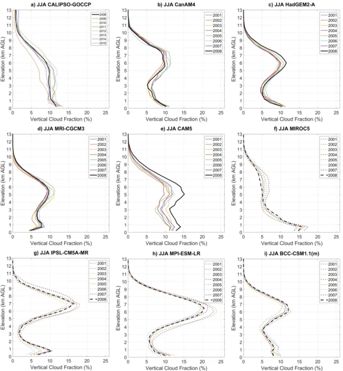
Starting with the first limitation—we acknowledge that using only a single year for comparisons could be a very serious limitation. In fact, the seriousness of this limitation depends on if the model biases are larger than the interannual variability. To evaluate the seri-ousness of this single-year limitation, we compare our single-year evaluation with a multiyear evaluation. Specifically, we compare winter and summer cloud fraction data for eight years (2008–15 for observations, 2001–08 for models) with those that were done for one year (Fig. 3). The results of this comparisonFigs. 7
and8reveal that the interannual variability of cloud fraction profiles over Greenland is less than 5% at all levels for all models except IPSL-CM5A-MR in win-ter. In the observations, the cloud fractions for the year 2008 are representative of the mean cloud fraction between 2008 and 2015; they are within62% or better at all heights. Thus, the model biases are larger than the interannual variability, at least for the models that we could assess.
Moving to the second, more fundamental limitation— we are not able to compare lidar cloud properties with direct surface radiation observations over all of Green-land. To address this observational limitation, we assess the relationship between cloud influence on surface ra-diation and cloud properties at the one location where both are available: Summit.
To assess if the relationships between cloud properties and radiation at Summit are relevant for the rest of the Greenland ice sheet, we compare cloud property biases over all of Greenland with those over just Summit (Tables 3and4). In winter, in many models, the sign of the cloud cover biases match over Greenland and Summit, but in two models (CanAM4 and HadGEM2-A) the sign of the biases differ. Compared to other models, the biases in CanAM4 and HadGEM2-A are small and can be due to regional differences in the two models. In summer, every model underestimates the cloud cover as well as the opaque and nonopaque cloud fraction. Only the cloud elevation biases are different; most of the time, the models underestimate the mean cloud altitude above Greenland and overestimate it at
Summit. The consistency of most of the cloud property biases between the Greenland average and Summit fosters the use of observations at Summit only. In the next section, we look in more detail at how the simulated cloud properties and radiative effects compare to the observations in the Summit environment only.
c. Evaluation of surface CRE in models using observations from Summit
We begin with winter because the lack of shortwave radiation during winter makes it simpler to relate cloud properties to cloud radiative effects. Indeed, the total CRE is equivalent to longwave cloud radiative effect (CRELW) during winter. The longwave flux at the surface
depends mostly on cloud and atmosphere properties with cloud cover being the main property affecting CRELW.
During winter, the monthly spaceborne-lidar cloud cover at Summit ranges between 40% and 80% (Fig. 9a). The corresponding monthly mean CRELWmeasured at Summit
ranges from130 to 150Wm22(Fig. 9b).
During winter at Summit, there are strong connections between model biases in the cloud properties (cover, opacity, altitude) and model biases in CRELW. We find
models with the smallest cloud cover have the smallest CRELW. For example, CAM5 is the model with the least
cloud cover, and it has a correspondingly small value of CRELW. Cloud cover bias and CRELWbias are not always
so simply related to each other. In fact, HadGEM2-A and CanAM4 have cloud cover between 50% and 80% but underestimate the CRELWby;210 W m22compared to
the ground observations, suggesting cloud properties in-fluence the CRELWbias in these two models.
Having investigated winter, we next move to summer. Evaluating model CRE and connecting model cloud property biases to model CRE biases is more complex in summer because we must consider both shortwave and longwave radiation. The shortwave CRE is influenced by the surface albedo and thus is measuring the cloud cooling but relative to the surface albedo. At Summit, the observed cloud cover and observed CRELWare both
larger in summer than in winter. During summer, the cloud cover ranges between 70% and 90% (Fig. 10a) and CRELWis 60 W m22(Fig. 10c).
During summer, clouds in the models do not radiatively warm the surface enough compared to the observations. In summer, this bias is larger than in winter for CanAM4 and HadGEM2-A because these two models do not re-produce the seasonal cycle of the cloud cover at Summit. In contrast, only CAM5 produces more cloud cover in summer than in winter. While CAM5 better reproduces the seasonal cycle, it still simulates too little summer cloud cover and thus underestimates the surface warming compared to observations.
Cloud cover biases explain most of the CRESWbiases:
The models with the smallest cloud cover, such as CAM5 (Fig. 10a), also produce the smallest shortwave cloud ra-diative cooling (Fig. 10d). While MRI-CGCM3 simulates just a bit more clouds than CAM5 in JJA (Fig. 10a), it overestimates the CRESWat the surface compared to
CAM5 and to ground observations. The two models
produce distinct shortwave forcing for the same cloud cover, with average values of CRESW, CAM55 23.7W m22
and CRESW, MRI-CGCM3 5 221.5 W m22 at Summit
(Fig. 10b).
In some cases as described above, the cloud cover alone does not explain all the CRESWbiases. Thus, next
we look at the other factors influencing the CRESW.
FIG. 7. Mean cloud fraction profile over Greenland calculated in DJF for (a) CALIPSO-GOCCP for the years 2008–15 and for (b)–(i) eight CMIP5 models for the years 2001–08.
Figure 11 suggests two other factors explain the dif-ference of CRESWbetween CAM5 and MRI-CGCM3:
1) More downward shortwave fluxes reach the sur-face in CAM5 compared to MRI-CGCM3 (150 W m22 in summer;Fig. 11c). It is likely because more opaque clouds are produced by MRI-CGCM3 compared to CAM5 (Fig. 4). 2) The surface albedos in summer are very different between the two models. In MRI-CGCM3,
the surface albedo reaches values as low as 0.73, whereas it stays above 0.8 in CAM5 (Fig. 11d). In the Summit ground observations, the average measured surface albedo is 0.86. A higher albedo leads to less shortwave radiative cooling due to the clouds, with all else constant. Thus, the very low albedo in MRI-CGCM3 helps to explain why its CRESW is so large even
though the model underestimates clouds. Hereafter,
T ABLE 3. Mean clo ud cove r, opaque and nono paque clo ud fract ion, and m ean clo ud altitud e over Green land and Su mmit in win ter. In the bra ckets, we indicat e the dif ferenc e betwe en the models and the ob servatio ns. The mean cloud altit ude is the mean alti tude of the base of ever y dete cte d cloud layer. Clo ud cove r (%) Opa que clo uds (%) Non opaque clouds (%) M ean cloud altit ude (km AGL ) Green land Sum mit G reenla nd Summi t Green land Sum mit G reenla nd Summi t Obse rvations 56 61 11 2 9 13 4.4 3.4 Model s CanA M4 55 (2 1) 68 (7) 14 (3) 14 (12) 12 (3) 24 (11) 4.1 (2 0.3) 4.9 (1.5) Had GEM2-A 51 (2 6) 66 (5) 11 (0) 5 (3) 7 (2 2) 14 (1) 3.9 (2 0.6) 4.9 (1.5) MR I-CGCM 3 40 (2 16) 44 (2 16) 8 (2 3) 2 (0) 7 (2 2) 11 (2 2) 3.7 (2 0.8) 4.9 (1.5) CAM 5 31 (2 25) 28 (2 33) 2 (2 9) 0 (2 2) 5 (2 4) 6 (2 7) 3.9 (2 0.5) 5.6 (2.2) MIR OC5 40 (2 16) 54 (2 7 ) —— ——— —— —3 .2 (2 1.2) 4 (0.6) IPSL-CM 5A-MR 63 (6) 73 (12) — — — — — — — — 6.2 (1.8) 8.1 (4.7) MPI-ES M-LR 61 (4) 74 (13) — — — — — — — — 4.6 (0.1) 6 (2.6) BCC _CSM 1.1(m ) 50 (2 7) 56 (2 5) — — — — — — — — 4.8 (0.4) 6 (2.6) T ABLE 4. As in Table 3 , bu t for summ er. Cloud cove r (%) Opaque cloud s (%) Non opaq ue cloud s (%) Mean cloud altit ude (km AGL ) Green land Su mmit Greenl and Summi t Greenl and Summ it Green land Summi t O bservati ons 64 — 80 — 29 — 15 — 16 — 33 — 4.5 — 3.6 — Model s C anAM 4 51 (2 13) 53 (2 27) 24 (2 5) 16 (1) 9 (2 8) 12 (2 21) 4.2 (2 0.3) 5.2 (1.7) H adGE M2-A 54 (2 10) 58 (2 21) 22 (2 7) 11 (2 4) 11 (2 5) 14 (2 19) 4.0 (2 0.5) 4.6 (1.0) M RI-CG CM3 44 (2 20) 40 (2 39) 15 (2 14) 5 (2 10) 5 (2 11) 10 (2 13) 3.8 (2 0.8) 5.0 (1.4) C AM5 39 (2 25) 34 (2 46) 6 (2 24) 0 (2 14) 12 (2 5) 17 (2 16) 3.9 (2 0.6) 5.5 (1.9) M IROC5 56 (2 8) 64 (2 16) — — — — — — — — 3.3 (2 1.2) 3.8 (0.2) IPS L-CM5 A-M R 39 (2 25) 43 (2 37) — — — — — — — — 5.4 (0.9) 7.3 (3.7) M PI-ES M-LR 58 (2 6) 68 (2 12) — — — — — — — — 5.4 (0.9) 6.6 (3.0) B CC_CS M1.1( m) 52 (2 12) 63 (2 17) — — — — — — — — 4.4 (2 0.1) 5.3 (1.8)
we looked at the contribution of these last two factors on the CRESW.
Using the surface shortwave flux outputs, we investi-gate how the average CRE in MRI-CGCM3 would change if the surface albedo and cloud opacity were changed (Fig. 11b). If the surface albedo in MRI-CGCM3 is in-creased to be similar to CAM5 (0.8 in July instead of 0.73), then CRESW, MRI-CGCM35 212 W m22in JJA indicating
that the difference in cloud opacity between the models explains (23.7) 2 (212) 5 8.3 W m22of their difference in CRESW. On the other hand, by theoretically decreasing
the cloud opacity such that MRI-CGCM3 matches CAM5, the downward shortwave fluxes become 400 W m22in July
instead of 350 W m22, and the remaining difference in CRESWis 7.8 W m22. Thus, cloud opacity and surface
albedo both contribute about half of the CRESW
difference between CAM5 and MRI-CGCM3. Combining the CRELW and CRESW components
reveals that the deficit of modeled longwave radia-tive warming compared to the ground observations is generally not compensated by the deficit of shortwave radiative cooling (Fig. 10b). Every model included in this study underestimates the net cloud radiative sur-face warming in summer. For the models with the best distribution of net CRE, this underestimation arises from compensating biases in longwave and shortwave
FIG. 9. Cloud cover and surface longwave radiative effect over Summit in winter. (a) PDF of the cloud cover from models and from satellite observations and (b) PDF of the surface longwave CRE from models and from ground-based observations. PDF are built from 28 3 28 gridbox monthly mean values for a bin size of 10% for the cloud cover and 10 W m22for CREsurf
LW. The number of sampled grid boxes (time and grid points) used for the calculation of
each PDF is given in brackets in the legend. This number depends on the model’s spatial resolution; the higher the resolution is, the higher is the number of sampled grid boxes. Cloud cover for the models comes from the model1 COSP/lidar.
components. In MRI-CGCM3, the clouds typically radiatively cool the surface as a result of its low surface albedo.
4. Discussion
Since we only have surface radiative flux measure-ments over Summit, the model surface radiation can only be evaluated over the Summit area (section 3c) and not over all Greenland. On the other hand, satellite observations provide an evaluation of the cloud cover, cloud fraction profile, and cloud opacity over all of Greenland; all these cloud variables influence the sur-face radiation.
Greenland cannot be seen as a homogeneous ice-covered area, and Summit might not be representative of other regions. For instance, in the ablation zones at the margin of Greenland, the ice albedo is lower com-pared to Summit (Goelles and Bøggild 2017). Over such low-albedo surfaces, decreasing cloud cover enhances
the surface melting (Hofer et al. 2017), when at the opposite, clouds’ presence can enhance the ice sheet melt in the middle of Greenland (Bennartz et al. 2013). These examples prove the necessity of having validated satellite observations above ice-covered surfaces. In the meantime, the Summit observations can be useful to evaluate models with the largest biases observed all over Greenland, including Summit.
The evaluation of the models showed that despite some constant biases, results may vary a lot from one model to another. Along with the clouds, the parame-terization of the Greenland ice sheet drives the vari-ability of the surface albedo and thus the CRE. Yet only few general circulation models are able to represent the surface of the Greenland ice sheet (Cullather et al. 2014). In future experiments, dynamic ice sheet models will be integrated in climate models (Eyring et al. 2016). This reflects that before the fifth assessment of the IPCC, Greenland received little attention from modeling centers. Further, cold clouds are hard to
FIG. 10. PDFs of cloud cover and surface radiation over Summit in summer for (a) cloud cover, (b) net cloud radiative effect, (c) LW cloud radiative effect, and (d) SW cloud radiative effect. PDFs are built from monthly mean values in 28 3 28 grid boxes located in the Summit region (z . 3000 m) in JJA 2008. The bin size of the PDF are values 10% for the cloud cover, 10 W m22for CREsurfLW, and 10 W m22for CREsurfSW. Values in the brackets of the legend indicate the number of sampled grid boxes (time and grid points) used for the calculation of each PDF. This number depends on the model’s spatial resolution; the higher the resolution is, the higher is the number of sampled grid boxes. Cloud cover for the four CMIP5 models comes from the COSP/lidar outputs.
model, and we lack observational constraint in the arctic regions.
To help constrain the models’ observational simulator are powerful tools. To improve the model evaluation of the cloud properties, the last CALIPSO-GOCCP opaque clouds diagnostics used in this study should be added in more climate models (Guzman et al. 2017). Hence, the evaluation of the cloud properties will be improved and help to understand the interactions between the clouds and the surface fluxes and thus help to predict future changes in the Greenland ice sheet mass balance.
5. Conclusions
In this study, we have evaluated climate model out-puts compared to CALIPSO and ground-based obser-vations in Greenland.
The comparison with CALIPSO observations re-vealed that the group of climate models examined here has some spread in their representation of vertical cloud fraction, cloud cover, and cloud opacity, with some constant biases in each model. Among the four models containing the height-intensity histogram outputs, they all underestimate the nonopaque clouds with large SR (SR . 30), and most models tend to underestimate opaque clouds observed in CALIPSO-GOCCP. These clouds are frequent in the observations, especially below 2 km AGL and are mostly liquid or mixed-phase clouds.
Biases in these cloud categories confirm the difficulty of the models to create liquid-containing clouds at tem-peratures below 08C (Cesana et al. 2012). On the other hand, some models create too many opaque clouds, es-pecially in summer. This may be a compensating error that reduces biases in Earth’s radiative budget (Nam et al. 2012).
The comparison to Summit observations revealed that the models underestimate the CRE at the surface es-pecially in summer. The CRE biases may be a conse-quence of the underestimated cloud cover in the models in summer (ranging from 246% to 221%). Fewer clouds causes an underestimation of the longwave ra-diative warming effect (235.7 to 213.6 W m22) and an underestimation of shortwave cooling effect (11.5 to 110.5 W m22) even though the model albedos are lower than that measured at Summit (’0.8 in the models and ’0.9 in the observations). Overall, the simulated clouds do not radiatively warm the surface as much as in the observations.
The effect this bias has on the CRE over Greenland during summer depends on the surface albedo. CanAM4 produces the most opaque clouds, but it creates them over high-albedo surfaces, while HadGEM2-A creates opaque clouds above surfaces with a low albedo (,0.7). Thus, for the same amount of simulated opaque clouds, the shortwave radiative cooling effect is higher in HadGEM2-A than in CanAM4.
FIG. 11. Simulated annual cycle of the (a) cloud cover, (b) surface SW CRE, (c) all sky downward shortwave flux, and (d) surface albedo as simulated by two CMIP5 climate models (CAM5 and MRI-CGCM3) over the Summit region (z. 3000 m) in 2008. The cloud cover is obtained from models 1 COSP/lidar. Solid lines are standard models and models1 COSP/lidar outputs, while the dotted lines in (b) are perturbed ones.
Since the overall cloud radiative warming is estimated in the models, we may expect an under-estimation of Greenland surface melting. However, misrepresentation of clouds is not the only contributor to biases in the modeled surface melting. Previous works have shown that near-surface temperature is colder in the models than in the reanalysis independently of cloud presence (Chapman and Walsh 2007). Indeed, the surface area over Greenland with a near-surface temperature around zero is two times smaller in the models than in the reanalysis (not shown). The extent to which cloud biases impact surface temperature biases requires further study. In this paper, we focused on the role of clouds on the surface melting, which is one side of the ice sheet mass balance; on the other side, the precipitations act as a source of mass. Precipitations are obviously connected to cloud presence so that satellites such as CloudSat and CALIPSO can contribute to the documentation of pre-cipitating clouds. Currently, studies based on model prediction suggest that more precipitation will fall in a warmer climate (Gregory and Huybrechts 2006;Fettweis et al. 2013). In future work, spaceborne radar combined with spaceborne lidar observations will enable a full as-sessment of the influence of clouds on surface melt and precipitation over Greenland.
Acknowledgments. The authors would like to ac-knowledge the support of NASA, CNES, and ClimServ for access to the CALIOP data. This work was sup-ported in part by the CNES/EECLAT project. JEK acknowledges funding support from NASA Grant 15-CCST15-0025. NBM and MDS acknowledge funding support from the U.S. National Science Foundation Grants PLR1303879 and PLR1314156. The authors thank the three anonymous reviewers who greatly helped to improve the manuscript.
REFERENCES
Arabelos, D., 2000: Intercomparisons of the global DTMs ETOPO5, TerrainBase and JGP95E. Phys. Chem. Earth, 25A, 89–93,https://doi.org/10.1016/S1464-1895(00)00015-6. Bennartz, R., and Coauthors, 2013: July 2012 Greenland melt
ex-tent enhanced by low-level liquid clouds. Nature, 496, 83–86,
https://doi.org/10.1038/nature12002.
Bodas-Salcedo, A., and Coauthors, 2011: COSP: Satellite simula-tion software for model assessment. Bull. Amer. Meteor. Soc., 92, 1023–1043,https://doi.org/10.1175/2011BAMS2856.1. ——, and Coauthors, 2014: Origins of the solar radiation biases
over the Southern Ocean in CFMIP2 models. J. Climate, 27, 41–56,https://doi.org/10.1175/JCLI-D-13-00169.1.
Cawkwell, F. G. L., and J. L. Bamber, 2002: The impact of cloud cover on the net radiation budget of the Greenland ice sheet. Ann. Glaciol., 34, 141–149,https://doi.org/10.3189/ 172756402781817789.
Cesana, G., and H. Chepfer, 2012: How well do climate models simulate cloud vertical structure? A comparison between CALIPSO-GOCCP satellite observations and CMIP5 models. Geophys. Res. Lett., 39, L20803, https://doi.org/10.1029/ 2012GL053153.
——, and ——, 2013: Evaluation of the cloud thermodynamic phase in a climate model using CALIPSO-GOCCP. J. Geophys. Res. Atmos., 118, 7922–7937,https://doi.org/10.1002/jgrd.50376. ——, J. E. Kay, H. Chepfer, J. M. English, and G. de Boer, 2012: Ubiquitous low-level liquid-containing Arctic clouds: New observations and climate model constraints from CALIPSO-GOCCP. Geophys. Res. Lett., 39, L20804, https://doi.org/ 10.1029/2012GL053385.
Chapman, W. L., and J. E. Walsh, 2007: Simulations of Arctic tem-perature and pressure by global coupled models. J. Climate, 20, 609–632,https://doi.org/10.1175/JCLI4026.1.
Chepfer, H., S. Bony, D. Winker, M. Chiriaco, J.-L. Dufresne, and G. Sèze, 2008: Use of CALIPSO lidar observations to evaluate the cloudiness simulated by a climate model. Geophys. Res. Lett., 35, L15704,https://doi.org/10.1029/2008GL034207.
——, ——, ——, G. Cesana, J. L. Dufresne, P. Minnis, C. J. Stubenrauch, and S. Zeng, 2010: The GCM-Oriented CALIPSO Cloud Product (CALIPSO-GOCCP). J. Geophys. Res., 115, D00H16,https://doi.org/10.1029/2009JD012251. ——, G. Cesana, D. Winker, B. Getzewich, M. Vaughan, and
Z. Liu, 2013: Comparison of two different cloud climatologies derived from CALIOP-attenuated backscattered measure-ments (level 1): The ST and the CALIPSO-GOCCP. J. Atmos. Oceanic Technol., 30, 725–744,https:// doi.org/10.1175/JTECH-D-12-00057.1.
Chiriaco, M., R. Vautard, H. Chepfer, M. Haeffelin, J. Dudhia, Y. Wanherdrick, Y. Morille, and A. Protat, 2006: The ability of MM5 to simulate ice clouds: Systematic comparison between simulated and measured fluxes and lidar/radar profiles at the SIRTA atmospheric observatory. Mon. Wea. Rev., 134, 897– 918,https://doi.org/10.1175/MWR3102.1.
Clough, S., M. Shephard, E. Mlawer, J. Delamere, M. Iacono, K. Cady-Pereira, S. Boukabara, and P. Brown, 2005: Atmo-spheric radiative transfer modeling: A summary of the AER codes. J. Quant. Spectrosc. Radiat. Transfer, 91, 233–244,
https://doi.org/10.1016/j.jqsrt.2004.05.058.
Cullather, R. I., S. M. J. Nowicki, B. Zhao, and M. J. Suarez, 2014: Evaluation of the surface representation of the Greenland ice sheet in a general circulation model. J. Climate, 27, 4835–4856,
https://doi.org/10.1175/JCLI-D-13-00635.1.
Dee, D. P., and Coauthors, 2011: The ERA-Interim reanalysis: Configuration and performance of the data assimilation sys-tem. Quart. J. Roy. Meteor. Soc., 137, 553–597,https://doi.org/ 10.1002/qj.828.
Dufresne, J.-L., and Coauthors, 2013: Climate change projections using the IPSL-CM5 Earth system model: From CMIP3 to CMIP5. Climate Dyn., 40, 2123–2165,https://doi.org/10.1007/ s00382-012-1636-1.
Eyring, V., S. Bony, G. A. Meehl, C. A. Senior, B. Stevens, R. J. Stouffer, and K. E. Taylor, 2016: Overview of the Coupled Model Intercomparison Project Phase 6 (CMIP6) experi-mental design and organization. Geosci. Model Dev., 9, 1937– 1958,https://doi.org/10.5194/gmd-9-1937-2016.
Fettweis, X., E. Hanna, C. Lang, A. Belleflamme, M. Erpicum, and H. Gallée, 2013: Brief communication ‘‘Important role of the mid-tropospheric atmospheric circulation in the recent surface melt increase over the Greenland ice sheet.’’ Cryosphere, 7, 241–248,https://doi.org/10.5194/tc-7-241-2013.
Giorgetta, M. A., and Coauthors, 2013: Climate and carbon cycle changes from 1850 to 2100 in MPI-ESM simulations for the Coupled Model Intercomparison Project phase 5. J. Adv. Model. Earth Syst., 5, 572–597,https://doi.org/10.1002/jame.20038. Goelles, T., and C. E. Bøggild, 2017: Albedo reduction of ice
caused by dust and black carbon accumulation: A model ap-plied to the K-transect, west Greenland. J. Glaciol., 63, 1063– 1076,https://doi.org/10.1017/jog.2017.74.
Gregory, J., and P. Huybrechts, 2006: Ice-sheet contributions to future sea-level change. Philos. Trans. Roy. Soc., 364A, 1709– 1732,https://doi.org/10.1098/rsta.2006.1796.
Griggs, J. A., and J. L. Bamber, 2008: Assessment of cloud cover characteristics in satellite datasets and reanalysis products for Greenland. J. Climate, 21, 1837–1849,https://doi.org/10.1175/ 2007JCLI1570.1.
Guzman, R., and Coauthors, 2017: Direct atmosphere opacity ob-servations from CALIPSO provide new constraints on cloud-radiation interactions. J. Geophys. Res. Atmos., 122, 1066–1085,
https://doi.org/10.1002/2016JD025946.
Hanna, E., and Coauthors, 2008: Increased runoff from melt from the Greenland ice sheet: A response to global warming. J. Climate, 21, 331–341,https://doi.org/10.1175/2007JCLI1964.1. Henderson, D. S., T. L’Ecuyer, G. Stephens, P. Partain, and M. Sekiguchi, 2013: A multisensor perspective on the radiative impacts of clouds and aerosols. J. Appl. Meteor. Climatol., 52, 853–871,https://doi.org/10.1175/JAMC-D-12-025.1.
Hofer, S., A. J. Tedstone, X. Fettweis, and J. L. Bamber, 2017: Decreasing cloud cover drives the recent mass loss on the Greenland ice sheet. Sci. Adv., 3, e1700584,https://doi.org/ 10.1126/sciadv.1700584.
Hurrell, J. W., and Coauthors, 2013: The Community Earth System Model: A framework for collaborative research. Bull. Amer. Meteor. Soc., 94, 1339–1360, https://doi.org/10.1175/ BAMS-D-12-00121.1.
Kalnay, E., and Coauthors, 1996: The NCEP/NCAR 40-Year Re-analysis Project. Bull. Amer. Meteor. Soc., 77, 437–471,https:// doi.org/10.1175/1520-0477(1996)077,0437:TNYRP.2.0.CO;2. Kato, S., N. G. Loeb, F. G. Rose, D. R. Doelling, D. A. Rutan, T. E.
Caldwell, L. Yu, and R. A. Weller, 2013: Surface irradiances consistent with CERES-derived top-of-atmosphere shortwave and longwave irradiances. J. Climate, 26, 2719–2740,https:// doi.org/10.1175/JCLI-D-12-00436.1.
Kay, J. E., L. Bourdages, N. B. Miller, A. Morrison, V. Yettella, H. Chepfer, and B. Eaton, 2016: Evaluating and improving cloud phase in the Community Atmosphere Model version 5 using spaceborne lidar observations. J. Geophys. Res. Atmos., 121, 4162–4176,https://doi.org/10.1002/2015JD024699. Klein, S. A., Y. Zhang, M. D. Zelinka, R. Pincus, J. Boyle, and
P. J. Gleckler, 2013: Are climate model simulations of clouds improving? An evaluation using the ISCCP simula-tor. J. Geophys. Res. Atmos., 118, 1329–1342,https://doi.org/ 10.1002/jgrd.50141.
Krabill, W., and Coauthors, 2004: Greenland ice sheet: Increased coastal thinning. Geophys. Res. Lett., 31, L24402, https:// doi.org/10.1029/2004GL021533.
Lacour, A., H. Chepfer, M. D. Shupe, N. B. Miller, V. Noel, J. Kay, D. D. Turner, and R. Guzman, 2017: Greenland clouds ob-served in CALIPSO-GOCCP: Comparison with ground-based summit observations. J. Climate, 30, 6065–6083,
https://doi.org/10.1175/JCLI-D-16-0552.1.
Martin, G. M., and Coauthors, 2011: The HadGEM2 family of Met Office Unified Model climate configurations. Geosci. Model Dev., 4, 723–757,https://doi.org/10.5194/gmd-4-723-2011.
Mernild, S. H., T. L. Mote, and G. E. Liston, 2011: Greenland ice sheet surface melt extent and trends: 1960–2010. J. Glaciol., 57, 621–628,https://doi.org/10.3189/002214311797409712. Miller, N. B., M. D. Shupe, C. J. Cox, V. P. Walden, D. D. Turner,
and K. Steffen, 2015: Cloud radiative forcing at Summit, Greenland. J. Climate, 28, 6267–6280,https://doi.org/10.1175/ JCLI-D-15-0076.1.
——, ——, ——, D. Noone, P. O. G. Persson, and K. Steffen, 2017: The surface energy budget responses to radiative forcing at Summit, Greenland. Cryosphere, 11, 497–516,https://doi.org/ 10.5194/tc-11-497-2017.
Morrison, A. L., J. E. Kay, H. Chepfer, R. Guzman, and V. Yettella, 2017: Isolating the liquid cloud response to recent Arctic sea ice loss using spaceborne lidar observations. J. Geophys. Res. At-mos., 123, 473–490,https://doi.org/10.1002/2017JD027248. Morrison, H., G. de Boer, G. Feingold, J. Harrington, M. D. Shupe,
and K. Sulia, 2012: Resilience of persistent Arctic mixed-phase clouds. Nat. Geosci., 5, 11–17,https://doi.org/10.1038/ ngeo1332.
Nam, C., S. Bony, J.-L. Dufresne, and H. Chepfer, 2012: The ‘too few, too bright’ tropical low-cloud problem in CMIP5 models. Geophys. Res. Lett., 39, L21801, https://doi.org/10.1029/ 2012GL053421.
National Geophysical Data Center, 1995: TerrainBase, global 5 arc-minute ocean depth and land elevation from the US National Geophysical Data Center (NGDC). National Center for Atmospheric Research, accessed 1 October 2014,http:// rda.ucar.edu/datasets/ds759.2.
Noel, V., and H. Chepfer, 2010: A global view of horizontally oriented crystals in ice clouds from Cloud-Aerosol Lidar and Infrared Pathfinder Satellite Observation (CALIPSO). J. Geophys. Res., 115, D00H23, https://doi.org/10.1029/ 2009JD012365.
Rignot, E., and P. Kanagaratnam, 2006: Changes in the velocity structure of the Greenland ice sheet. Science, 311, 986–990,
https://doi.org/10.1126/science.1121381.
Shupe, M. D., 2011: Clouds at Arctic atmospheric observato-ries. Part II: Thermodynamic phase characteristics. J. Appl. Meteor. Climatol., 50, 645–661, https://doi.org/10.1175/ 2010JAMC2468.1.
——, and J. M. Intrieri, 2004: Cloud radiative forcing of the Arctic surface: The influence of cloud properties, surface albedo, and solar zenith angle. J. Climate, 17, 616–628, https://doi.org/ 10.1175/1520-0442(2004)017,0616:CRFOTA.2.0.CO;2. ——, and Coauthors, 2013: High and dry: New observations of
tropospheric and cloud properties above the Greenland ice sheet. Bull. Amer. Meteor. Soc., 94, 169–186,https://doi.org/ 10.1175/BAMS-D-11-00249.1.
Solomon, A., M. D. Shupe, and N. B. Miller, 2017: Cloud–atmospheric boundary layer–surface interactions on the Greenland ice sheet during the July 2012 extreme melt event. J. Climate, 30, 3237– 3252,https://doi.org/10.1175/JCLI-D-16-0071.1.
Stephens, G. L., and Coauthors, 2002: The CloudSat mission and the A-Train: A new dimension to space-based observations of clouds and precipitation. Bull. Amer. Meteor. Soc., 83, 1771– 1790,https://doi.org/10.1175/BAMS-83-12-1771.
Stubenrauch, C. J., and Coauthors, 2013: Assessment of global cloud datasets from satellites: Project and database initiated by the GEWEX radiation Panel. Bull. Amer. Meteor. Soc., 94, 1031–1049,https://doi.org/10.1175/BAMS-D-12-00117.1. Taylor, K. E., R. J. Stouffer, and G. A. Meehl, 2012: An overview of
CMIP5 and the experiment design. Bull. Amer. Meteor. Soc., 93, 485–498,https://doi.org/10.1175/BAMS-D-11-00094.1.
Tedesco, M., X. Fettweis, M. R. van den Broeke, R. S. W. van de Wal, C. J. P. P. Smeets, W. J. van de Berg, M. C. Serreze, and J. E. Box, 2011: The role of albedo and accumulation in the 2010 melting record in Greenland. Environ. Res. Lett., 6, 014005,
https://doi.org/10.1088/1748-9326/6/1/014005.
——, ——, T. Mote, J. Wahr, P. Alexander, J. E. Box, and B. Wouters, 2013: Evidence and analysis of 2012 Greenland records from spaceborne observations, a regional climate model and reanalysis data. Cryosphere, 7, 615–630, https:// doi.org/10.5194/tc-7-615-2013.
Van Tricht, K., and Coauthors, 2016: Clouds enhance Greenland ice sheet meltwater runoff. Nat. Commun., 7, 10266,https:// doi.org/10.1038/ncomms10266.
Vaughan, D. G., and Coauthors, 2013: Observations: Cryosphere. Climate Change 2013: The Physical Science Basis, T. F. Stocker et al., Eds., Cambridge University Press, 317–382,http://www. ipcc.ch/pdf/assessment-report/ar5/wg1/WG1AR5_Chapter04_ FINAL.pdf.
Von Salzen, K., and Coauthors, 2013: The Canadian Fourth Gen-eration Atmospheric Global Climate Model (CanAM4). Part I: Representation of physical processes. Atmos.–Ocean, 51, 104–125,https://doi.org/10.1080/07055900.2012.755610. Watanabe, M., and Coauthors, 2010: Improved climate simulation
by MIROC5: Mean states, variability, and climate sensitivity. J. Climate, 23, 6312–6335,https://doi.org/10.1175/2010JCLI3679.1. Winker, D.M., J. R. Pelon, and M. P. McCormick, 2003: The CALIPSO mission: Spaceborne lidar for observation of aero-sols and clouds. Proc. SPIE, 4893, 3–5,https://doi.org/10.1117/ 12.466539.
Wu, T., and Coauthors, 2014: An overview of BCC climate system model development and application for climate change studies. J. Meteor. Res., 28, 34–56,https://doi.org/10.1007/s13351-014-3041-7. Yukimoto, S., and Coauthors, 2012: A new global climate model of
the Meteorological Research Institute: MRI-CGCM3—Model description and basic performance. J. Meteor. Soc. Japan, 90A, 23–64,https://doi.org/10.2151/jmsj.2012-A02.