HAL Id: hal-03008876
https://hal.univ-grenoble-alpes.fr/hal-03008876
Submitted on 17 Nov 2020
HAL is a multi-disciplinary open access archive for the deposit and dissemination of sci-entific research documents, whether they are pub-lished or not. The documents may come from teaching and research institutions in France or
L’archive ouverte pluridisciplinaire HAL, est destinée au dépôt et à la diffusion de documents scientifiques de niveau recherche, publiés ou non, émanant des établissements d’enseignement et de recherche français ou étrangers, des laboratoires
Seismic Body Waves With Ocean Wave Climate and
Microseism Sources
Lei Li, Pierre Boué, Lise Retailleau, Michel Campillo
To cite this version:
Lei Li, Pierre Boué, Lise Retailleau, Michel Campillo. Spatiotemporal Correlation Analysis of Noise-Derived Seismic Body Waves With Ocean Wave Climate and Microseism Sources. Geochemistry, Geophysics, Geosystems, AGU and the Geochemical Society, 2020, 21 (9), �10.1029/2020GC009112�. �hal-03008876�
1
Spatiotemporal correlation analysis of noise-derived seismic body waves with ocean
2
wave climate and microseism sources
3 4
Lei Li1,2, Pierre Boué2, Lise Retailleau3,4, Michel Campillo2 5
1State Key Laboratory of Earthquake Dynamics, Institute of Geology, CEA, Beijing 100029, China
6
2Univ. Grenoble Alpes, Univ. Savoie Mont Blanc, CNRS, IRD, IFSTTAR, ISTerre, 38000 Grenoble, France
7
3Université de Paris, Institut de physique du globe de Paris, CNRS, F-75005 Paris, France
8
4Observatoire Volcanologique du Piton de la Fournaise, Institut de physique du globe de Paris, F-97418 La Plaine des Cafres,
9
France
10 11
Corresponding author: Lei Li (lilei@ies.ac.cn)
12 13
Key Points: 14
Time variations of a noise-derived P-type phase are compared with those of the ocean 15
wave heights and microseism sources. 16
Do not equate a positive correlation with a causal relation when studying the links 17
between noise sources and noise-derived signals. 18
The derivation of seismic signals from ambient noise relies on the competition between 19
the effective and ineffective sources. 20
21
Abstract 22
Seismic signals can be extracted from ambient noise wavefields by the correlation technique. 23
Recently, a prominent P-type phase was observed from teleseismic noise correlations in the 24
secondary microseism period band. The phase is named Pdmc in this paper, corresponding to its
25
origin from the interference between the Direct P waves transmitting through the deep Mantle 26
and the Core (P and PKPab waves). We extract the phase by correlating noise records from two 27
seismic networks in the northern hemisphere, and locate the microseism sources that are efficient 28
for the Pdmc construction in the south Pacific. We investigate the spatiotemporal links of the Pdmc
29
signal with global oceanic waves and microseism sources. Interestingly, the correlation with 30
wave height is higher in several regions surrounding the effective source region, rather than in 31
the effective source region. The Pdmc amplitude is highly correlated with the power of the
32
effective microseism sources. Also, it is apparently correlated with ineffective sources in the 33
southern hemisphere, and anti-correlated with sources in the northern hemisphere. We ascribe 34
the correlation with the ineffective southern sources to the spatiotemporal interconnections of the 35
southern sources. The anti-correlation with northern sources can be explained by the reverse 36
seasonal patterns between the southern and northern sources, and by that the northern sources 37
impede the signal construction. The signal construction from noise correlations relies on the 38
competition between the effective and ineffective sources, not just on the power of the effective 39
sources. This principle should be valid in a general sense for noise-derived signals. 40
41
Plain Language Summary 42
Earth is experiencing tiny but incessant movement induced by natural forces, particularly, storm-43
driven ocean waves. While this ambient seismic noise (microseism) was deemed a nuisance in 44
the past, it can be turned into signals via the seismic correlation technique. 45
Recently, a new P-type phase was derived from the noise correlations between two regional 46
seismic networks. The noise-derived phase originates from the correlation between P waves that 47
propagate through the deep mantle and outer core of the Earth. 48
The temporal amplitude variations of the noise-derived signals are compared with the variations 49
of microseism sources in the oceans. We show that the signal emergence depends on the 50
competition between the sources in a specific region that contribute to the signals and sources in 51
other regions. The conclusion can be generalized to other noise-derived seismic phases. 52
We also analyze the links of the noise-derived signals to ocean waves. In our case, the ocean 53
waves in the contributing source region are dominated by wind seas forced by local winds, 54
whereas the excitation of microseisms is primarily owing to the freely traveling swells generated 55
by oceanic storms in surrounding regions. 56
57
1 Introduction 58
The incessant background vibrations of Earth had been observed as early as the birth of 59
seismometers in the later 19th century (Bernard, 1990; Dewey & Byerly, 1969; Ebeling, 2012). 60
They were termed “microseisms” due to their tiny amplitudes. With more apparatus deployed 61
worldwide, it was soon recognized that microseisms are ubiquitous and irrelevant to seismicity. 62
The observation of microseisms aroused interests from various disciplines. Researchers linked 63
the generation of microseisms to atmosphere processes and ocean wave activity. Meteorologists 64
tried to employ land observations of microseisms to track remote oceanic storms (e.g., Harrison, 65
1924). Since the mid-twentieth century, it has been well known that microseisms are excited by 66
storm-driven ocean waves. The most energetic microseisms that dominate the seismic noise 67
spectra, namely, the so-called secondary microseisms at seismic periods around 7 s (Peterson, 68
1993), are excited by the nonlinear interactions between nearly equal-frequency ocean waves 69
propagating in nearly opposite directions (Longuet-Higgins, 1950; Hasselmann, 1963). The 70
periods of the excited secondary microseisms are half those of the colliding ocean waves. The 71
excitation source is equivalent to a vertical pressure applied to the water surface, which is 72
proportional to the product of the heights of the opposing equal-frequency waves. Due to this 73
second order relation, moderate sea states can sometimes generate loud microseism noise 74
(Obrebski et al., 2012). Thus, the presence of a strong microseism event does not necessarily 75
imply a locally intense sea state. 76
By coupling the excitation theory of secondary microseisms proposed by Longuet-77
Higgins (1950) with the ocean wave action model, Kedar et al. (2008) modeled the secondary 78
microseism excitations in the north Atlantic, and validated the numerical modeling by comparing 79
with inland seismological observations. Afterwards, more authors simulated the oceanic 80
microseism sources and some reported the consistency between predictions and observations 81
(e.g., Ardhuin et al., 2011, 2015; Hillers et al., 2012; Stutzmann et al., 2012; Nishida & Takagi, 82
2016). Stopa et al. (2019) compared the microseism simulations with real observations to 83
validate their corrections to the global reanalysis wind fields, which systematically reduced the 84
residuals in the wave hindcast over the past decades. 85
The seismic excitation by an oceanic microseism source is essentially akin to that by an 86
earthquake, in that the seismic wavefield recorded at any point is a convolution of the source 87
time function with the Green function of the propagating medium between source and receiver. 88
Their main difference lies in the source process. For earthquakes, the sudden rupture of faults 89
leads to short-duration, impulsive source time functions. Isolated seismic phases are generally 90
distinguishable from the seismograms. In contrast, the excitation of microseisms, approximated 91
as Gaussian random process by some authors (Peterson, 1993; Steim, 2015), is incessant, leading 92
to long, random-like source time functions. The convolution mixture signals are not directly 93
discernible from the seismograms. With array beamforming (Rost & Thomas, 2002) or 94
correlation technique (Campillo & Paul, 2003; Shapiro & Campillo, 2004), specific phases from 95
distant microseism sources have been identified from microseism noise records (e.g., Gerstoft et 96
al., 2008; Landès et al., 2010; Zhang et al., 2010; Euler et al., 2014; Reading et al., 2014; Gal et 97
al., 2015; Liu et al., 2016; Nishida & Takagi, 2016; Meschede et al., 2017, 2018; Retailleau & 98
Gualtieri, 2019). The correlation technique is advantageous in that, by correlating the noise 99
records at two receivers, explicit seismic signals can be derived. Noise-derived surface waves 100
have been used to infer the azimuthal and seasonal changes of noise sources (e.g., Stehly et al., 101
2006). Noise-derived body waves can provide better constrains in imaging the noise sources 102
(Landès et al., 2010). Recently, deep body waves that propagate through the mantle and core 103
have been extracted from ambient noise (e.g., Boué et al., 2013; Lin et al., 2013; Nishida, 2013; 104
Poli et al., 2015; Xia et al., 2016; Spica et al., 2017; Retailleau et al., 2020). The noise-derived 105
body waves are valuable for surveying the deep structure and for understanding the links 106
between seismological observations and atmospheric/oceanographic phenomena. 107
Hillers et al. (2012) made the first global-scale comparison between the oceanic 108
microseism sources derived from seismological observations and oceanographic modeling. The 109
seismologically derived data (time resolution: 13 days; spatial resolution: 2.5° latitude 5° 110
longitude) are the global back-projections of near-zero-lag P signals generated from the cross 111
correlations of microseism P waves at seismic array (Landès et al., 2010). The modeled data 112
(time resolution: 3 hours; spatial resolution: 1° latitude 1.25° longitude) are a global extension 113
of the numerical simulation by Kedar et al. (2008). The two datasets are resampled to common 114
resolutions for comparison. For the seismologically derived data, the back-projection is based on 115
the relationship between the source-receiver distance and the horizontal slowness of teleseismic 116
P wave. However, seismic phases that have common slownesses (e.g., P and PP waves) cannot 117
be discriminated in this method (Gerstoft et al., 2008; Landès et al., 2010). Thus, the imaged 118
sources are somewhat ambiguous. For the modeled data, coastal reflections of ocean waves, that 119
can play a role in the ocean wave-wave interactions at near-coast regions (Longuet-Higgins, 120
1950; Ardhuin et al., 2011), are neglected. Due to the resonance of seismic waves in the water 121
columns, bathymetry can have significant effect on the excitation of microseisms (Longuet-122
Higgins, 1950; Kedar et al., 2008; Hillers et al., 2012). The importance to account for the 123
bathymetric effect on the microseism P-wave excitations has been addressed in several studies 124
(e.g., Euler et al., 2014; Gal et al., 2015; Meschede et al., 2017). Hillers et al. (2012) considered 125
the bathymetric effect, but using the amplification factors derived by Longuet-Higgins (1950) for 126
surface waves. 127
Rascle and Ardhuin (2013) established an oceanographic hindcast database that includes 128
global oceanic secondary microseism sources of a 3-hour time resolution and a 0.5° spatial 129
resolution. Coastal reflections were accounted for in the modeling (Ardhuin et al., 2011). 130
Regarding the bathymetric effect on microseism excitations, Gualtieri et al. (2014) proposed the 131
formulae for body waves based on ray theory. Concerning the localization of noise sources, Li et 132
al. (2020) developed a double-array method that can estimate the respective slownesses of the 133
interfering waves, and thereby, provide better constrains for the determination of the correlated 134
seismic phases. The microseism sources that are effective for the derivation of seismic signals 135
from noise records, can be mapped by back-projecting the noise-derived signals along the ray 136
paths of the correlated phases. The double-array configuration eliminates the ambiguity in 137
determining the effective source region (Fresnel zone). In this study, we integrate these new 138
progresses to survey the associations of noise-derived body waves to ocean wave activity and 139
microseism excitations. 140
This paper is organized as follows. In section 2, we review the main results of Li et al. 141
(2020) who reported the observation of a prominent P-type phase from the noise correlations 142
between two regional seismic networks at teleseismic distance. The noise-derived phase has its 143
spectral content concentrated in the period band of the secondary microseisms that are excited by 144
the nonlinear ocean wave-wave interactions. In this paper, we denote the phase as Pdmc,
145
corresponding to the fact that the phase originates from the correlation between the Direct P 146
waves that transmit through the deep Mantle and the outer Core (microseism P and PKPab 147
waves). In section 3, we estimate the temporal variations in the Pdmc amplitude and refute the
148
associations to seismicity. In section 4, correlation analysis is used to unveil the spatiotemporal 149
links of the Pdmc signal with the global oceanic wave climate and microseism sources. Last, we
150
discuss the significance of this study in seismology, oceanography and climate science. 151
2 Noise-derived Pdmc phase
152
Li et al. (2020) correlated the seismic noise records from two regional seismic networks 153
at teleseismic distance: the FNET array in Japan and the LAPNET array in Finland (Fig. 1a). The 154
continuous seismograms were divided into 4 h segments and whitened in the frequency domain. 155
Segments with large spikes (like earthquakes) were discarded. The available segments of each 156
FNET-LPANET station pairs were correlated. For more technical details, see section 2 of Li et 157
al. (2020). From the vertical-vertical components of the FNET-LAPNET noise correlations, they 158
observed coherent spurious arrivals (the Pdmc phase named in the previous section) that emerged
159
~200 s earlier than the direct P waves (Fig. 1b). By estimating the respective slownesses of the 160
interfering waves and their time delay, it is unveiled that a quasi-stationary phase interference 161
between the teleseismic P waves at FNET and the PKPab waves at LAPNET, emanating from 162
noise sources in the ocean south of New Zealand (NZ), lead to the noise-derived Pdmc phase (Fig.
163
1c). The quasi-stationary phase condition refers to that the interfering waves have no common 164
path or common slowness, but the stack of correlation functions over a range of sources can still 165
be constructive as an effect of finite frequency. This observation contrasts with the strict 166
stationary phase condition that has been employed by Phạm et al. (2018) to explain the spurious 167
body phases in the earthquake coda correlations. The strict condition implies the existence of 168
sources in the stationary-phase region, or say, the correlated waves have common ray paths or 169
common slownesses. Li et al. (2020) substantiates the explanation of quasi-stationary phase for 170
the observed Pdmc signals with numerical experiments based on ray theory and based on
spectral-171
element modeling, and highlighted the discrepancies between (microseism) noise correlations 172
and coda correlations. 173
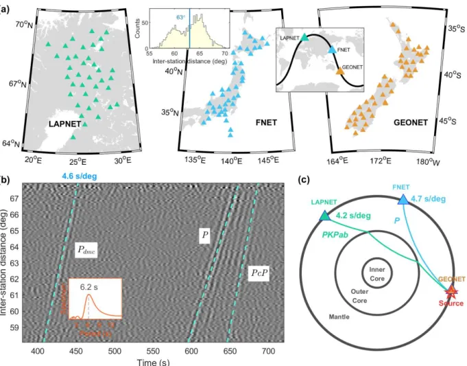
The Pdmc phase has an apparent slowness of 4.6 s/deg, while the slownesses of the
174
interfering P and PKPab waves are 4.7 s/deg and 4.2 s/deg, respectively. The dominant period of 175
the Pdmc phase is 6.2 s, typical for secondary microseisms. The observation of the Pdmc phase is
176
time-asymmetric (Fig. S1a). Its absence from the mirror side is ascribed to the faintness of the 177
corresponding source in the low-latitude Atlantic (Fig. S1b). 178
There are several advantages to investigating the links between noise-derived signals and 179
microseism sources with the Pdmc phase. First, the correlated P and PKPab waves are both
180
prominent phases in the ballistic microseism wavefields. The Pdmc phase is easily observable
181
from noise correlations, even between some single station pairs and on some single days (Fig. 182
S2). Second, the isolation of Pdmc signals avoids potential bias caused by other prominent
183
signals. Third, the effective sources are confined in a limited, unique region (Fresnel zone). In 184
contrast, noise-derived surface waves have a broad Fresnel zone around the line across the 185
correlated stations, and noise-derived P waves can have multiple Fresnel zones (see fig. 5 of 186
Boué et al., 2014 for instance). The uniqueness of the effective source region can facilitate the 187
study on the correlation between the noise-derived signals and the effective sources. Fourth, the 188
correlated FNET and LAPNET networks are next to the northern Pacific and Atlantic, 189
respectively, while the effective source region locates in the southern Pacific. The northern 190
oceans have consistent seasonal variation pattern distinct from (reverse to) that of the southern 191
oceans (Stehly et al., 2006; Stutzmann et al., 2009; Landès et al., 2010; Hillers et al., 2012; 192
Reading et al., 2014; Turners et al., 2020). These geographical configurations make the 193
observations easier to interpret. Last, there happens to be a seismic array (GEONET) in NZ next 194
to the effective source region for the Pdmc phase. The seismic data from GEONET provide extra
195
support to our study. 196
198
Figure 1. (a) Three regional broadband seismic networks used in this study: left, the LAPNET 199
array in Finland (38 stations); center, the FNET array in Japan (41 stations); right, the GEONET 200
array in New Zealand (46 stations). The histogram inset shows the distribution of the separation 201
distances between the 1558 FNET-LAPNET station pairs. The center-to-center distance is 63° 202
between LAPNET and FNET, and 85° between FNET and GEONET. The global inset shows the 203
geographical locations of the three networks that are aligned on a great circle (dark line). (b) 204
Annual FNET-LAPNET noise correlations that are filtered between 5 s and 10 s and stacked 205
over time and in 0.1° inter-station distance bins. The spectrum inset indicates that the Pdmc phase
206
has a 6.2 s peak period. (c) Ray paths of the interfering waves that generate the Pdmc phase. The
207
effective source region is close to GEONET. 208
3 Temporal variations 209
We extract the temporal variations of the Pdmc signals by beamforming the
FNET-210
LAPNET noise correlations on a daily basis. The daily noise correlations are shifted and stacked 211
by 212
𝐵(𝑡) = 〈𝐶 𝑡 + 𝑑 − 𝑑 ∙ 𝑝 〉, (1) 213
with 〈∙〉 the mean operator, 𝐶 and 𝑑 the correlation function and the distance between the ith 214
FNET station and the jth LAPNET station, 𝑑 the reference distance (63°), 𝑝 the apparent 215
slowness of the Pdmc phase (4.6 s/deg), and 𝑡 the time. The image in Fig. 2 shows the envelopes
216
of the daily beams computed from the Hilbert transform of Eq. (1), with the daily Pdmc strength
217
by averaging the envelope amplitudes plotted in the top panel. The strength of daily Pdmc signals
218
varies strikingly, extremely strong on some single days (see the labeled dates in the Pdmc strength
219
curve for examples), but indiscernible on most other days. 220
Considering that the region of effective source is tectonically active, one should 221
investigate the plausible connection between the Pdmc signals and seismicity. From Fig. 2, it is
222
obvious that Pdmc is decorrelated with the NZ seismicity. Also, it shows no connection with
223
global large earthquakes as has been observed for coda-derived core phases at periods of 20 to 50 224
s (Lin & Tsai, 2013; Boué et al., 2014). That again demonstrates the substantial difference 225
between ambient noise correlations and earthquake coda correlations, as emphasized by Li et al. 226
(2020). The Pdmc strength exhibits an obvious pattern of seasonal variation. The seasonal pattern
227
does not favor a tectonic origin because of the lack of a seasonal pattern in seismicity. Instead, an 228
oceanic origin is more favored because of the well-documented fact that oceanic wave activity 229
and microseism excitations show similar seasonal pattern: more powerful during the local winter 230
(e.g., Stehly et al., 2006; Stutzmann et al., 2009; Landès et al., 2010; Hillers et al., 2012; Reading 231
et al., 2014). Next, we analyze the correlations between Pdmc signals and oceanographic data at a
232
global scale. 233
234
Figure 2. Temporal variations in the strength of daily Pdmc signals, in comparisons with the daily
235
cumulative seismic moments in NZ (pink line at bottom; for earthquake magnitudes above 2.0 in 236
GEONET catalogue) and global large earthquakes (stars; magnitudes above 7.0 in USGS 237
catalogue; see Table S1 for a full list of earthquakes in 2008 above magnitude 5.5). The 238
background image is composed of columns of daily envelopes of beamed FNET-LAPNET noise 239
correlations. Darker color represents larger amplitude. The curve on the top shows the daily Pdmc
240
strength derived from the daily envelopes. Dates of the three largest peaks are labeled. 241
4 Correlation analysis 242
The sea state is composed of ocean waves at various frequencies and propagation 243
directions. The nonlinear interaction between nearly equal-frequency ocean waves traveling in 244
nearly opposite directions is equivalent to a vertical random pressure applied to the ocean surface 245
(Longuet-Higgins, 1950; Hasselmann, 1963), so that microseisms are generated. Figure 3(a) 246
shows a global map of average Power Spectral Density (PSD) of the equivalent surface pressure 247
for a seismic period of 6.2 s, during the northern winter months of 2008. The hindcast PSD data 248
are simulated by Ardhuin et al. (2011) and Rascle & Ardhuin (2013), based on the microseism 249
excitation theory of Longuet-Higgins (1950) and Hasselmann (1963). The most energetic 250
microseism excitations occur in the northern Atlantic south of Greenland and Iceland (near 251
LAPNET), and in the northern Pacific between Japan and Alaska (near FNET). Figure 3(b) 252
shows the map for the austral winter months, with the strongest excitations occurring between 253
NZ and Antarctic (near GEONET). The seasonal pattern of oceanic microseism excitations 254
results from the same pattern of global wave climate (Figs 3e-f). The seasonal pattern of the Pdmc
255
strength agrees with that of the microseism excitation and wave climate in the effective source 256
region south of NZ. 257
We compute the correlation coefficient (denoted as r) between the Pdmc strength and the
258
source PSDs at each grid point, and thereby obtain a global correlation map (Fig. 3c). The largest 259
r value for Pdmc and source PSD arises at [47°S, 177°E] in the effective source region (E in Fig.
260
3c). The corresponding time series of daily source PSDs is plotted in Fig. 4, in parallel with the 261
Pdmc strength. Large peaks in the Pdmc series have good correspondence with large peaks in the
262
source PSD series. From Fig. 3(c), one can observe a broad region of positive r values (red 263
colors; roughly, south Atlantic, south Pacific, and Indian ocean). However, the positive 264
correlation does not imply a causality between the Pdmc phase and the sources outside the
265
effective region E. We ascribe the apparent positive correlation to the spatial correlation of the 266
time-varying microseism excitation. As shown in Fig. 3(d), the source at [47°S, 177°E] in region 267
E exhibits a similar pattern of apparent correlations with global sources as in Fig. 3(c). Despite 268
the microseism excitations at varying locations are independent (Hasselmann, 1963), we note 269
that the independence refers only to the phase information. The time variations of microseism 270
source power are spatially associated. That is not surprising since the interacting ocean waves 271
that excite microseisms could be driven by the same storms and swells can propagate freely over 272
thousands of kilometers away (Ardhuin et al., 2009). We also notice there are high-r regions that 273
may not be fully explained by the spatial association. These regions are characterized by low 274
intensity of microseism excitations in Figs 3(a-b). A striking example is around [12°N, 88°E] in 275
the Bay of Bengal (F in Fig. 3c). From Fig. 4, it can be seen that the source PSD series for 276
[12°N, 88°E] is dominated by a single peak around May 1st, coincident with the largest P dmc
277
peak. This coincidence leads to a high value of correlation coefficient. However, the Bay of 278
Bengal is far away from the FNET-LAPNET great circle, which is inconsistent with the source 279
imaging shown later in Fig. 5. Thus, the high correlation is spurious and does not imply a 280
causality relationship between the microseism sources in the Bay of Bengal and the Pdmc signals.
281
Figures 3(g-h) show the correlation maps for hs, which will be discussed later.
As shown in Fig. 4, prominent peaks in the Pdmc series have correspondence in the source
283
PSD series for the effective source at [47°S, 177°E]. However, there are some peaks in the latter 284
without correspondence in the former (see the labeled dates in Fig. 4b for examples). Note that 285
here the Pdmc strength is compared to the microseism source PSD at single point in Fig. 4,
286
whereas the effective sources spread over a region. One needs to verify if the peak disparities 287
observed from Figs 4(a-b) can be ascribed to the neglect of the spreading of the effective source 288
region. To evaluate an overall microseism excitation in the effective source region, the 289
bathymetric effect on P-wave excitation should be considered (in the previous analysis for single 290
point locations, the consideration of bathymetric effect is unnecessary because a scaling over the 291
source PSD series does not change the value of the correlation coefficient between Pdmc and
292
source PSD). Using the equations proposed by Gualtieri et al. (2014) and the bathymetry around 293
NZ (Fig. 5a), we compute the bathymetric amplification factors for P waves at a period of 6.2 s 294
(Fig. 5b; see Fig. S3 for comparisons between the factors calculated following Longuet-Higgins, 295
1950 and Gualtieri et al., 2014). The factors vary largely with locations. Also, note that the Pdmc
296
phase has different sensitivity to the sources in the effective region, or say, the sources make 297
varying contributions to the Pdmc signal. The power of sources should be weighted in the
298
averaging. We obtain the weights by back-projecting the beam power of noise correlations onto a 299
global grid (Fig. 5c; see Supplementary for technical details). Figure 5(d) shows the map of 300
annually averaged source PSDs surrounding NZ and Fig. 5(e) shows the map after the 301
modulation of the bathymetric amplification factors in Fig. 5(b). The spatial patterns are altered 302
significantly, indicating the importance to account for the bathymetric effect. The final source 303
imaging that has been weighted by Fig. 5(c), is plotted in Fig. 5(f). It agrees well with the 304
effective source region E determined from the correlation map in Fig. 3(c). Replacing the annual 305
PSD map in Fig. 5(d) with daily PSD maps, we obtain maps like Fig. 5(f) for each date. 306
Averaging over the map leads to the time series of daily intensity in the effective source region 307
(labeled as effective source intensity in Fig. 6). Averaging over a wide region has the advantage 308
that the effects of potential source location errors due to the simplification of Earth model for fast 309
travel time calculation, which have been addressed in some single array back-projection studies 310
(e.g., Gal et al., 2015; Nishida & Takagi, 2016), can be largely reduced. From Fig. 6, one can see 311
that the new effective source intensity series has almost the same peaks as the source PSD series 312
for [47°S, 177°E] in Fig. 4(b), suggesting that the observed peak disparities are caused by other 313
reasons. Next, we investigate if the disparities are caused by errors in the simulation of hindcast 314
data or if there are other physical explanations. 315
The microseism source PSD data are simulated from the hindcast data of ocean wave 316
directional spectra base on the excitation theory of Longuet-Higgins (1950) and Hasselmann 317
(1963), which have no constrains from seismological observations. One should consider the 318
accuracy of the simulation: can we ascribe the peak disparities in Fig. 4 to the simulation error or 319
not? The seismic noise records from the GEONET array adjacent to the effective source region 320
provide the opportunity to validate the simulation. To obtain the daily microseism noise levels at 321
GEONET, we apply the Hampel filter, a variant of the classic median filter, to the continuous 322
seismograms to discard earthquakes and anomalous impulses. The filter replaces outliers with 323
the medians of the outliers’ neighbors and retains the normal samples. Technical details are 324
provided in section S4 of the Supplementary. The resultant GEONET noise level exhibits a good 325
correlation with the effective source intensity (r = 0.7). We thus deem that the numerical 326
simulations are statistically reliable. When the effective source intensity is high, the GEONET 327
noise level should also be high (see the peaks marked by dots in Fig. 6 for examples). However, 328
due to the great spatiotemporal variability of noise sources in the effective region and the 329
complexity of seismic waves propagating from ocean to land (Ying et al., 2014; Gualtieri et al., 330
2015), a larger peak in the source intensity series does not necessarily imply a larger peak in the 331
noise level time series (e.g., see diamonds in Fig. 6 for examples). We also emphasize that a high 332
GEONET noise level does not need to always have a correspondence in the source intensity (see 333
squares in Fig. 6 for example), because the GEONET stations record microseisms emanating 334
from noise sources all around, not only from the effective source region. 335
The above analysis explains the observed disparities between the Pdmc strength and the
336
effective source intensity. From Fig.6, one can see that the disparities primarily emerge in the 337
shaded period when dominant microseism sources shift to the north hemisphere. The shading 338
roughly separates the northern winter from the austral winter. The correlation between Pdmc
339
strength and effective source intensity is low in the shaded period (r = 0.16), in contrast to the 340
high correlation during the unshaded period (r = 0.74). Large Pdmc peaks always emerge on dates
341
during the austral winter when the effective source intensity is much higher than its median, and 342
meanwhile, noise levels at FNET and LAPNET are below their respective medians (see dots in 343
Fig. 6 for examples). The seasonal variations of oceanic sources in the southern hemisphere are 344
less strong than in the northern hemisphere (Fig. 3). On some dates (see triangles in Fig. 6 for 345
examples), the effective source intensity can be considerable, but relevant Pdmc peaks are still
346
missing. We notice that the corresponding microseism levels at FNET and LAPNET are 347
obviously above their medians. Intensive ocean activity and microseism excitations in the north 348
Pacific and Atlantic, lead to increased microseism noise levels at FNET and LAPNET. The Pdmc
349
strength is anticorrelated with microseism noise levels at FNET (r = 0.12) and LAPNET (r = -350
0.18). We hereby conjecture that the microseism energy from the distant effective source region 351
is dwarfed by the energetic microseisms excited by oceanic sources closer to the correlated 352
FNET and LAPNET arrays, and consequently, Pdmc signals are overwhelmed by the background
353
noise in the FNET-LAPNET cross-correlations. Last, we mention that the median threshold in 354
Fig. 6 separates the major features of the time series described above, but there is no guarantee 355
that it is a perfect threshold due to the nonlinear relationships between the Pdmc strength and the
356
noise levels at the arrays. 357
359
Figure 3. (a) Global map of average PSD of oceanic microseism sources in 2008 northern winter 360
months (Jan. to Mar. and Oct. to Dec.), for a seismic perod of 6.2 s. (b) Similar to (a) but for 361
2008 austral winter months (Apr. to Sep.). (c) Correlation map (corrmap) for the Pdmc strength
362
and global microseism noise sources. Circles mark two regions with highest correlation 363
coefficients: E, effective source region surrounding [47°S, 177°E] south of NZ; F, fake highly-364
correlated region surrouding [12°N, 88°E] in the Bay of Bengal. (d) Correlation map for the 365
source at [47°S, 177°E] and global sources. (e) Mean significant wave height (hs; four times the
366
square root of the zeroth-order moment of ocean-wave frequency spectrum) in northern winter 367
months. (f) Similar to (e) but for austral winter months. (g) Correlation map for the Pdmc strength
368
and global wave heights. (h) Correlation map for wave heights at [47°S, 177°E] and global wave 369
heights. The oceanographical hindcast data are provided by the IOWAGA products (Rascle & 370
Ardhuin, 2013). 371
373
Figure 4. True correlation (r = 0.73) between (a) the Pdmc strength from Fig. 2 and (b) the power
374
of source at [47°S, 177°E] in the effective source region (E in Fig. 3c), and spurious correlation 375
(r = 0.71) between Pdmc and (c) the power of source at [12°N, 88°E] in the Bay of Bengal (F in
376
Fig. 3c). 377
379
Figure 5. (a) Bathymetry around NZ. (b) Bathymetric amplification factors for P-type waves. 380
(c) Imaging of effective sources obtained from the back-projection of the FNET-LAPNET noise 381
correlations. (d) Annual average of source PSDs in 2008. (e) Source PSDs in (d) modulated by 382
the factors in (b). (f) Source PSDs in (e) further modulated by the weights in (c). 383
385
Figure 6. Temporal variations of daily Pdmc strength, microseism noise levels at three networks,
386
and average wind speeds, wave heights and microseism excitations in the effective source 387
region. The curves are normalized by their own maximums. Dashed horizontal lines denote their 388
respective medians. Symbols mark some dates cited in the main text. When computing the 389
effective source intensity, the bathymetric factors in Fig. 5(b) and weights in Fig. 5(c) are used. 390
When computing the average wind speeds and wave heights, weights in Fig. 5(c) are used. 391
5 Discussions and conclusions 392
In this study, we explore the relations between the noise-derived Pdmc signals and global
393
oceanic microseism sources using spatiotemporal correlation analysis. The effective source 394
region E for the Pdmc phase is successfully identified from the correlation map in Fig. 3(c), which
395
is consistent with that determined from the seismological back-projection in Fig. 5(c). The 396
correlation map provides a convenient way to identify the effective sources of noise-derived 397
seismic signals. 398
In our case, the seismic networks used for noise correlation are located in the northern 399
hemisphere, while the effective source region is in the southern hemisphere. Ideally, we expect a 400
correlation map with the following features: positive correlation with sources in the effective 401
region, and negative or insignificant correlations with other inefficient sources. Positive 402
correlation indicates a contribution to the construction of Pdmc signal from noise correlations,
403
negative correlation implies an adverse impact, and insignificant correlation (decorrelation) 404
means a negligible effect on the signal construction. However, we obtained a correlation map 405
roughly showing that, the Pdmc signal is correlated with the southern sources and anti-correlated
406
with the northern sources. The correlation with southern sources outside the effective region can 407
be interpreted with the spatiotemporal correlation of the power of the microseism sources in the 408
southern oceans, due to the large span of ocean storms and the long-range propagation of swells. 409
The anti-correlation with the northern sources, can partly be explained by the well-known 410
reverse seasonal patterns of oceanic microseism excitations in the south and north hemispheres 411
(Stutzmann et al., 2009; Landès et al., 2010; Hillers et al., 2012; Reading et al., 2014). Another 412
important reason is that compared to the remote effective sources in the south hemisphere, the 413
northern sources closer to the correlated stations have larger impacts on the microseism noise 414
levels at stations. Strong energy flux from the northern sources outshines the microseism energy 415
coming from the distant effective sources. That deteriorates the construction of the Pdmc phase.
416
The noise-derived Pdmc signals are primarily observable in the austral winter. That can be, on one
417
hand, attributed to the stronger effective source intensity during that period, and on the other 418
hand, to the relative tranquility in the northern oceans. 419
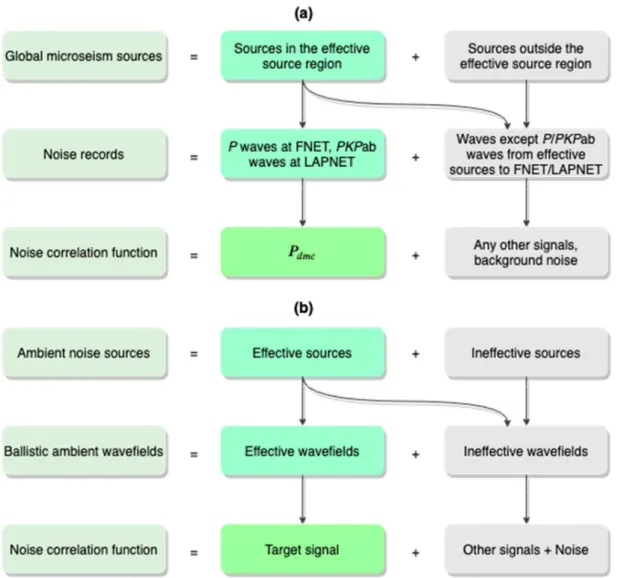
In Fig. 7, we summarize the classification of noise sources, the decomposition of 420
wavefields, and the associations to the constituents of the inter-receiver noise correlation 421
function. The diagram of Fig. 7(a) explains the relationships using the case study of the Pdmc
422
phase discussed above. We generalize Fig. 7(a) to the derivation of an arbitrary signal (referred 423
to as the target signal for convenience) from ambient noise wavefields (Fig. 7b). The noise 424
correlation function is composed of the target signal, any other signals and background noise. A 425
source or a wave is called effective if it contributes to the construction of the target signal from 426
noise correlations. Otherwise, it is called ineffective. The construction of the target signal is 427
exclusively ascribed to the interference between the effective waves. Stronger effective sources 428
(relative to ineffective sources) imply more effective waves in the total wavefield, and thereby, a 429
better quality for the noise-derived target signal. Note that not all waves emanating from the 430
effective sources, but only those following specific ray paths, are effective. There might be 431
multiple pairs of seismic phases that could contribute to the construction of the target signal. 432
However, their relative strength matters. As for the case of the Pdmc phase, the effective waves
433
are P and PKPab, which are both prominent phases in the ballistic wavefield. Li et al. (2020) 434
showed that the PcP-PKPab correlation and the PcS-PcPPcP correlation, could also lead to a 435
signal at around the Pdmc emerging time. However, the PcP, PcS, and PcPPcP waves are weak
436
phases in the ballistic wavefield, and thereby have minor contributions to the Pdmc signals. We
437
emphasize that the sketch in Fig. 7(b) is only suitable for the ambient noise wavefields that are 438
dominated by ballistic waves. 439
From Fig. 6, one can observe a high correlation between wind speed and wave height in 440
region E (r = 0.74). It indicates that the ocean waves in region E are likely dominated by the 441
waves forced by local winds. The correlation between wave height and microseism excitation is 442
low (r = 0.25), implying a dominant role of the freely propagating swells in exciting the 443
microseisms. Extreme sea state does not guarantee strong microseism excitation. That is not 444
surprising according to the microseism excitation theory (Hasselmann, 1963; Longuet-Higgins, 445
1950): the excitation is proportional to the product of the heights of the colliding equal-frequency 446
ocean waves. In lack of equal-frequency waves coming from opposite directions, even extreme 447
wave climate cannot incite strong secondary microseisms. In contrast, for large peaks in the 448
microseism excitation, the corresponding wave heights are generally moderate (e.g., on May 1st 449
and 23rd). On these two dates, the low wind speeds but moderate wave heights in region E 450
suggest that the ocean waves are dominantly the freely travelling swells from elsewhere, as also 451
illustrated in the supplementary movie S1. Oppositely propagating equal-frequency swells 452
collide with each other and incite strong microseisms. Our analysis and observations agree with 453
those of Obrebski et al. (2012), who investigated a specific case that small swells from two 454
storms meeting in the eastern Pacific generate loud microseism noise. There are also examples 455
showing that wind waves can play a role in the excitation of microseisms, for instance, around 456
July 31st when the local winds, wave height, and microseism excitations are all strong. Such 457
examples are few. The good consistency between the temporal variations in the Pdmc strength, the
458
effective source intensity and the NZ microseism noise level (Fig. 6), provides extra supports to 459
the analysis of the Pdmc observations and the quasi-stationary phase arguments proposed by Li et
460
al. (2020). It also gives credits to the validity of the numerical modeling of oceanic microseism 461
sources by Ardhuin et al. (2011) and Rascle & Ardhuin (2013). 462
We have described above the implications of this study in seismology and in 463
understanding the process of microseism excitation. Now, we discuss the significance in 464
oceanography and climate science. Well-documented historical ocean storms and wave climate 465
are valuable for improving our understanding of climate change and global warming (Ebeling 466
2012). However, modern satellite observations of ocean waves and storms have a history of 467
merely decades. Microseisms are induced by storm-driven ocean waves (Ardhuin et al., 2015; 468
Hasselmann, 1963; Longuet-Higgins, 1950). The records of microseisms contain the imprint of 469
climate (Aster et al., 2010; Stutzmann et al., 2009). Instrumental observation of microseisms has 470
an over-century history, and started much earlier than the modern observations of ocean waves 471
and storms. It has been a long-lasting effort for the seismological community to digitalize the 472
historical analog seismograms (Bogiatzis & Ishii, 2016; Lecocq et al., 2020). Researchers expect 473
that past seismic records can be used to recover undocumented historical ocean storms and wave 474
climate (Ebeling 2012; Lecocq et al., 2020). 475
This study confirms that it is possible to detect remote microseism events (burst of 476
microseism energy) with land observation of microseisms. We demonstrate that the noise-477
derived Pdmc signals can be employed to monitor microseism events in a specific ocean region
478
(Fig. 5). The remote monitoring of microseisms is promising as an aid to improving wave 479
hindcast, in similar manners as demonstrated by Stopa et al. (2019). The comparative analysis in 480
Fig. 6 indicates that the remote event detection could be effective in the absence of strong 481
sources near the stations, otherwise the detection could fail. Stations at low latitudes where wave 482
climate and microseism excitation are relatively mild, or inland stations far from oceans, should 483
have better performance in remote monitoring. 484
Energetic microseism excitation does not always need extreme in situ wave heights, and 485
extreme wave heights do not necessarily produce powerful microseisms (Obrebski et al., 2012; 486
and this study). It imply that secondary microseism events are not a perfect proxy for the 487
extremal in situ wave climate. However, it does not mean the long-lasting attempt to monitor 488
remote sea state and ocean storms with land observation of secondary microseisms is futile. In 489
the Pdmc-hs correlation map (Fig. 3g), the largest r values do not fall in the effective region E as
490
in the Pdmc-source correlation map (Fig. 3c), but in surrounding regions with moderate to high
491
ocean wave activity (the bounded areas in Fig. 3g). We speculate that these regions could be the 492
birthplaces of the colliding swells that generate the secondary microseisms in region E, or the 493
ocean waves in these regions are driven by the same storms as the colliding waves in region E 494
(see the spatial links of hs from Fig. 3h and supplementary movie S1). The detection of a
495
microseism event could affirm the existence of the causative storms that generated the ocean 496
waves propagating to the location of the microseism event, although the storms could be distant 497
from the events. 498
499
500
Figure 7. (a) Sketch explanation for the relationships between microseism noise sources and the 501
noise-derived Pdmc signal. (b) Generalization of diagram (a) for an arbitrary signal derived from
502
ambient noise wavefields that are dominated by ballistic waves. 503
Acknowledgments and data 504
The seismic data of FNET and LAPNET were provided by the National Research 505
Institute for Earth Science and Disaster Resilience (http://www.fnet.bosai.go.jp/; last access: 506
June 2018) and the Réseau Sismologique & Géodésique Français (http://www.resif.fr/; last 507
access: June 2018), respectively. The seismic data of GEONET and the earthquake catalogue of 508
New Zealand were provided by the GEONET Data Center (https://www.geonet.org.nz/; last 509
access: June 2018). The global earthquake catalogue was provided by the U.S. Geological 510
Survey (https://earthquake.usgs.gov/; last access: June 2018). The wind hindcast data were 511
provided by the European Centre for Medium-Range Weather Forecasts 512
(https://www.ecmwf.int/; last access: June 2018). The hindcast data of wave heights and 513
microseism source PSDs were provided by the IOWAGA products (Rascle & Ardhuin, 2013). 514
The bathymetry data were extracted from ETOPO1 Global Relief Model (Amante & Eakins, 515
2009). The computations were performed mainly on the ISTerre cluster. This work was 516
supported by Labex OSUG@2020 (Investissements d’avenir-ANR10LABX56) and the Simone 517
and Cino del Duca Foundation, Insitut de France. The authors acknowledge the support from the 518
European Research Council (ERC) under the European Union’s Horizon 2020 research and 519
innovation program (grant agreement No 742335, F-IMAGE). We also acknowledge Anya M. 520
Reading and an anonymous reviewer for their valuable reviews that helped to improve the clarity 521
of our paper, and special thanks to the editor for allowing the deadline extension during the 522
COVID-19 pandemic. 523
References 524
Amante, C., & Eakins, B. W. (2009). ETOPO1 1 Arc-Minute Global Relief Model: Procedures, 525
Data Sources and Analysis. NOAA Technical Memorandum NESDIS NGDC-24. 526
https://doi.org/10.7289/V5C8276M 527
Ardhuin, F., Chapron, B., & Collard, F. (2009). Observation of swell dissipation across oceans. 528
Geophysical Research Letters, 36(6), L06607. https://doi.org/10.1029/2008GL037030 529
Ardhuin, F., Stutzmann, E., Schimmel, M., & Mangeney, A. (2011). Ocean wave sources of 530
seismic noise. Journal of Geophysical Research: Oceans, 116(9), 1–21. 531
https://doi.org/10.1029/2011JC006952 532
Ardhuin, F., Gualtieri, L., & Stutzmann, E. (2015). How ocean waves rock the Earth: Two 533
mechanisms explain microseisms with periods 3 to 300s. Geophysical Research Letters, 534
42(3), 765–772. https://doi.org/10.1002/2014GL062782 535
Aster, R. C., McNamara, D. E., & Bromirski, P. D. (2010). Global trends in extremal microseism 536
intensity. Geophysical Research Letters, 37(14), 1–5. 537
https://doi.org/10.1029/2010GL043472 538
Bernard, P. (1990). Historical sketch of microseisms from past to future. Physics of the Earth 539
and Planetary Interiors, 63(3–4), 145–150. https://doi.org/10.1016/0031-9201(90)90013-540
N 541
Bogiatzis, P., & Ishii, M. (2016). DigitSeis: A New Digitization Software for Analog 542
Seismograms. Seismological Research Letters, 87(3), 726–736. 543
https://doi.org/10.1785/0220150246 544
Boué, P., Poli, P., Campillo, M., Pedersen, H., Briand, X., & Roux, P. (2013). Teleseismic 545
correlations of ambient seismic noise for deep global imaging of the Earth. Geophysical 546
Journal International, 194(2), 844–848. https://doi.org/10.1093/gji/ggt160 547
Boué, P., Poli, P., Campillo, M., & Roux, P. (2014). Reverberations, coda waves and ambient 548
noise: Correlations at the global scale and retrieval of the deep phases. Earth and 549
Planetary Science Letters, 391, 137–145. https://doi.org/10.1016/j.epsl.2014.01.047 550
Campillo, M., & Paul, A. (2003). Long-Range Correlations in the Diffuse Seismic Coda. 551
Science, 299(5606), 547–549. https://doi.org/10.1126/science.1078551 552
Dewey, J., & Byerly, P. (1969). The early history of Seismometry (to 1900). Bulletin of the 553
Seismological Society of America, 59(1), 183–227. 554
Ebeling, C. W. (2012). Inferring Ocean Storm Characteristics from Ambient Seismic Noise. In 555
R. Dmowska (Ed.), Advances in Geophysics (Vol. 53, pp. 1–33). Elsevier. 556
https://doi.org/10.1016/B978-0-12-380938-4.00001-X 557
Euler, G. G. G., Wiens, D. D. A., & Nyblade, A. A. (2014). Evidence for bathymetric control on 558
the distribution of body wave microseism sources from temporary seismic arrays in 559
Africa. Geophysical Journal International, 197(3), 1869–1883. 560
https://doi.org/10.1093/gji/ggu105 561
Gal, M., Reading, A. M., Ellingsen, S. P., Gualtieri, L., Koper, K. D., Burlacu, R., et al. (2015). 562
The frequency dependence and locations of short-period microseisms generated in the 563
Southern Ocean and West Pacific. Journal of Geophysical Research: Solid Earth, 120(8), 564
5764–5781. https://doi.org/10.1002/2015JB012210 565
Gerstoft, P., Shearer, P. M., Harmon, N., & Zhang, J. (2008). Global P, PP, and PKP wave 566
microseisms observed from distant storms. Geophysical Research Letters, 35(23), 4–9. 567
https://doi.org/10.1029/2008GL036111 568
Gualtieri, L., Stutzmann, E., Farra, V., Capdeville, Y., Schimmel, M., Ardhuin, F., & Morelli, A. 569
(2014). Modelling the ocean site effect on seismic noise body waves. Geophysical 570
Journal International, 197(2), 1096–1106. https://doi.org/10.1093/gji/ggu042 571
Gualtieri, L., Stutzmann, E., Capdeville, Y., Farra, V., Mangeney, A., & Morelli, A. (2015). On 572
the shaping factors of the secondary microseismic wavefield. Journal of Geophysical 573
Research B: Solid Earth, 120(9), 6241–6262. https://doi.org/10.1029/2000GC000119 574
Harrison, E. P. (1924). Microseisms and Storm Forecasts. Nature, 114(2870), 645–645. 575
https://doi.org/10.1038/114645b0 576
Hasselmann, K. (1963). A statistical analysis of the generation of microseisms. Reviews of 577
Geophysics, 1(2), 177–210. https://doi.org/10.1029/RG001i002p00177 578
Hillers, G., Graham, N., Campillo, M., Kedar, S., Landès, M., & Shapiro, N. (2012). Global 579
oceanic microseism sources as seen by seismic arrays and predicted by wave action 580
models. Geochemistry, Geophysics, Geosystems, 13(1), Q01021. 581
https://doi.org/10.1029/2011GC003875 582
Kedar, S., Longuet-Higgins, M., Webb, F., Graham, N., Clayton, R., & Jones, C. (2008). The 583
origin of deep ocean microseisms in the North Atlantic Ocean. Proceedings of the Royal 584
Society A: Mathematical, Physical and Engineering Sciences, 464(2091), 777–793. 585
https://doi.org/10.1098/rspa.2007.0277 586
Landès, M., Hubans, F., Shapiro, N. M., Paul, A., & Campillo, M. (2010). Origin of deep ocean 587
microseisms by using teleseismic body waves. Journal of Geophysical Research: Solid 588
Earth, 115(5), 1–14. https://doi.org/10.1029/2009JB006918 589
Lecocq, T., Ardhuin, F., Collin, F., & Camelbeeck, T. (2020). On the Extraction of Microseismic 590
Ground Motion from Analog Seismograms for the Validation of Ocean-Climate Models. 591
Seismological Research Letters. https://doi.org/10.1785/0220190276 592
Li, L., Boué, P., & Campillo, M. (2020). Observation and explanation of spurious seismic signals 593
emerging in teleseismic noise correlations. Solid Earth, 11(1), 173–184. 594
https://doi.org/10.5194/se-11-173-2020 595
Lin, F. C., & Tsai, V. C. (2013). Seismic interferometry with antipodal station pairs. Geophysical 596
Research Letters, 40(17), 4609–4613. https://doi.org/10.1002/grl.50907 597
Lin, F. C., Tsai, V. C., Schmandt, B., Duputel, Z., & Zhan, Z. (2013). Extracting seismic core 598
phases with array interferometry. Geophysical Research Letters, 40(6), 1049–1053. 599
https://doi.org/10.1002/grl.50237 600
Liu, Q., Koper, K. D., Burlacu, R., Ni, S., Wang, F., Zou, C., et al. (2016). Source locations of 601
teleseismic P, SV, and SH waves observed in microseisms recorded by a large aperture 602
seismic array in China. Earth and Planetary Science Letters, 449, 39–47. 603
https://doi.org/10.1016/j.epsl.2016.05.035 604
Longuet-Higgins, M. S. (1950). A Theory of the Origin of Microseisms. Philosophical 605
Transactions of the Royal Society A: Mathematical, Physical and Engineering Sciences, 606
243(857), 1–35. https://doi.org/10.1098/rsta.1950.0012 607
Meschede, M., Stutzmann, E., Farra, V., Schimmel, M., & Ardhuin, F. (2017). The Effect of 608
Water Column Resonance on the Spectra of Secondary Microseism P Waves. Journal of 609
Geophysical Research: Solid Earth, 122(10), 8121–8142. 610
https://doi.org/10.1002/2017JB014014 611
Meschede, M., Stutzmann, E., & Schimmel, M. (2018). Blind source separation of temporally 612
independent microseisms. Geophysical Journal International, 216(2), 1260–1275. 613
https://doi.org/10.1093/gji/ggy437 614
Nishida, K. (2013). Global propagation of body waves revealed by cross-correlation analysis of 615
seismic hum. Geophysical Research Letters, 40(9), 1691–1696. 616
https://doi.org/10.1002/grl.50269 617
Nishida, K., & Takagi, R. (2016). Teleseismic S wave microseisms. Science, 353(6302), 919– 618
921. https://doi.org/10.1126/science.aaf7573 619
Obrebski, M. J., Ardhuin, F., Stutzmann, E., & Schimmel, M. (2012). How moderate sea states 620
can generate loud seismic noise in the deep ocean. Geophysical Research Letters, 39(11), 621
1–6. https://doi.org/10.1029/2012GL051896 622
Phạm, T. S., Tkalčić, H., Sambridge, M., & Kennett, B. L. N. (2018). Earth’s Correlation 623
Wavefield: Late Coda Correlation. Geophysical Research Letters, 45(7), 3035–3042. 624
https://doi.org/10.1002/2018GL077244 625
Peterson, J. (1993). Observations and Modeling of Seismic Background Noise. U.S. Geol. Surv. 626
Open File Report 93-322. https://doi.org/10.3133/ofr93322 627
Poli, P., Thomas, C., Campillo, M., & Pedersen, H. A. (2015). Imaging the D″ reflector with 628
noise correlations. Geophysical Research Letters, 42(1), 60–65. 629
https://doi.org/10.1002/2014GL062198 630
Rascle, N., & Ardhuin, F. (2013). A global wave parameter database for geophysical 631
applications. Part 2: Model validation with improved source term parameterization. 632
Ocean Modelling, 70, 174–188. https://doi.org/10.1016/j.ocemod.2012.12.001 633
Reading, A. M., Koper, K. D., Gal, M., Graham, L. S., Tkalčić, H., & Hemer, M. A. (2014). 634
Dominant seismic noise sources in the Southern Ocean and West Pacific, 2000-2012, 635
recorded at the Warramunga Seismic Array, Australia. Geophysical Research Letters, 636
41(10), 3455–3463. https://doi.org/10.1002/2014GL060073 637
Retailleau, L., Boué, P., Li, L., & Campillo, M. (2020). Ambient seismic noise imaging of the 638
lowermost mantle beneath the North Atlantic Ocean. Geophysical Journal International, 639
222(2), 1339-1351. 640
Retailleau, L., & Gualtieri, L. (2019). Toward high-resolution period-dependent seismic 641
monitoring of tropical cyclones. Geophysical Research Letters, 46(3), 1329–1337. 642
https://doi.org/10.1029/2018GL080785 643
Rost, S., & Thomas, C. (2002). Array seismology: Methods and applications. Reviews of 644
Geophysics, 40(3), 1008. https://doi.org/10.1029/2000RG000100 645
Shapiro, N. M., & Campillo, M. (2004). Emergence of broadband Rayleigh waves from 646
correlations of the ambient seismic noise. Geophysical Research Letters, 31(7), 8–11. 647
https://doi.org/10.1029/2004GL019491 648
Spica, Z., Perton, M., & Beroza, G. C. (2017). Lateral heterogeneity imaged by small-aperture 649
ScS retrieval from the ambient seismic field. Geophysical Research Letters, 44(16), 650
8276–8284. https://doi.org/10.1002/2017GL073230 651
Stehly, L., Campillo, M., & Shapiro, N. M. (2006). A study of the seismic noise from its long-652
range correlation properties. Journal of Geophysical Research, 111(B10), B10306. 653
https://doi.org/10.1029/2005JB004237 654
Steim, J. M. (2015). Theory and Observations - Instrumentation for Global and Regional 655
Seismology. In Treatise on Geophysics (pp. 29–78). Elsevier. 656
https://doi.org/10.1016/B978-0-444-53802-4.00023-3 657
Stopa, J. E., Ardhuin, F., Stutzmann, E., & Lecocq, T. (2019). Sea state trends and variability: 658
consistency between models, altimeters, buoys, and seismic data (1979‐2016). Journal of 659
Geophysical Research: Oceans, 2018JC014607. https://doi.org/10.1029/2018jc014607 660
Stutzmann, E., Ardhuin, F., Schimmel, M., Mangeney, A., & Patau, G. (2012). Modelling long-661
term seismic noise in various environments. Geophysical Journal International, 191(2), 662
707–722. https://doi.org/10.1111/j.1365-246X.2012.05638.x 663
Stutzmann, E., Schimmel, M., Patau, G., & Maggi, A. (2009). Global climate imprint on seismic 664
noise. Geochemistry, Geophysics, Geosystems, 10(11), Q11004. 665
https://doi.org/10.1029/2009GC002619 666
Turner, R. J., Gal, M., Hemer, M. A., & Reading, A. M. (2020). Impacts of the Cryosphere and 667
Atmosphere on Observed Microseisms Generated in the Southern Ocean. Journal of 668
Geophysical Research: Earth Surface, 125(2). https://doi.org/10.1029/2019JF005354 669
Xia, H. H., Song, X., & Wang, T. (2016). Extraction of triplicated PKP phases from noise 670
correlations. Geophysical Journal International, 205(1), 499–508. 671
https://doi.org/10.1093/gji/ggw015 672
Ying, Y., Bean, C. J., & Bromirski, P. D. (2014). Propagation of microseisms from the deep 673
ocean to land. Geophysical Research Letters, 41(18), 6374–6379. 674
https://doi.org/10.1002/2014GL060979 675
Zhang, J., Gerstoft, P., & Shearer, P. M. (2010). Resolving P-wave travel-time anomalies using 676
seismic array observations of oceanic storms. Earth and Planetary Science Letters, 677
292(3–4), 419–427. https://doi.org/10.1016/j.epsl.2010.02.014 678
680
[Geochemistry, Geophysics, Geosystems]
681
Supporting Information for
682
Spatiotemporal correlation analysis of noise-derived seismic body waves with ocean wave
683
climate and microseism sources
684
Lei Li1,2, Pierre Boué2, Lise Retailleau3,4, Michel Campillo2 685
1State Key Laboratory of Earthquake Dynamics, Institute of Geology, CEA, Beijing 100029, China
686
2Univ. Grenoble Alpes, Univ. Savoie Mont Blanc, CNRS, IRD, IFSTTAR, ISTerre, 38000 Grenoble, France
687
3Université de Paris, Institut de physique du globe de Paris, CNRS, F-75005 Paris, France
688
4Observatoire Volcanologique du Piton de la Fournaise, Institut de physique du globe de Paris, F-97418 La Plaine des
689
Cafres, France
690 691
Contents of this file 692 693 Text S1 to S4 694 Figures S1 to S4 695 696
Additional Supporting Information (Files uploaded separately) 697
698
Caption for Table S1
699
Caption for Movie S1
700 701
Text S1. FNET-LAPNET noise correlations 702
The correlation function CAB between two seismograms (SA and SB) is given by
703
𝐶 (𝜏) = ∑ ( ) ( )
∑ ( ) ∑ ( )
. (S1) 704
The resultant CAB consists of an acausal part and a causal part, that correspond to the negative
705
lags (𝜏 < 0) and the positive lags (𝜏 > 0), respectively. For efficiency, it is routine to compute 706
the correlation function with the Fast Fourier Transform: 707
𝐶 (𝜏) =ℱ [ℱ( )ℱ∗( )]
∑ ( ) ∑ ( )
. (S2) 708
Figure S1(a) shows the acausal and causal sections of FNET-LAPNET noise correlations in 2008 709
that are filtered between 5 s and 10 s and binned in distance intervals of 0.1°. The acausal section 710
is flipped to share the time axis with the causal section. The expected locations of the acausal and 711
causal noise sources are marked by stars on the maps of global microseism source PSDs and 712
ocean wave heights in Fig. S1(b). The ocean wave activities and microseism excitations at the 713
acausal source region are intense, while those in the causal source region are fainter. 714
Consequently, the Pdmc phase is only observable from the acausal noise correlations.
715 716
717
Figure S1. (a) Acausal and causal sections of FNET-LAPNET noise correlations in 2008. (b) 718
Global maps of 6.2 s period secondary microseism sources and significant wave heights in 2008. 719
720
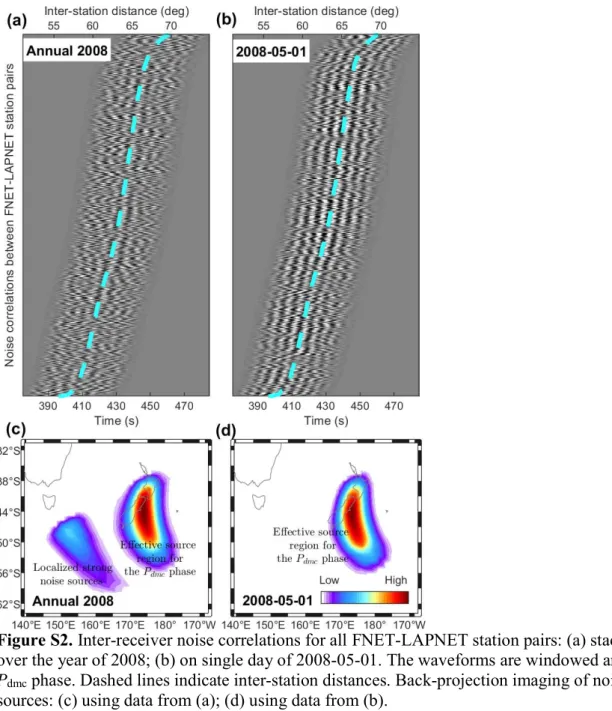
Text S2. Noise source imaging by back-projection 721
Assuming the interferometry between P waves at FNET and PKPab waves at LAPNET, we 722
image the effective noise sources through the back-projection of the FNET-LAPNET noise 723
correlations. We beam the FNET-LAPNET noise correlations and assign the beam power 724
𝑃 = 〈〈 𝐶 𝑡 + 𝑡 − 𝑡 〉 〉 , (S3) 725
onto a 0.5° 0.5° grid as the probabilities of noise sources on the global surface. In the above 726
equation, 〈∙〉 means the average over 𝑥, 𝐶 is the correlation function between the i-th FNET 727
station and the j-th LAPNET station, 𝑡 is the traveltime of the P wave from the s-th grid point 728
to the i-th FNET station, and 𝑡 is the traveltime of the PKPab waves from the s-th source to the 729
j-th LAPNET station. The inter-station noise correlations are windowed before the beamforming 730
(Fig. S2a). The noise source imaging for the annually stacked noise correlations is plotted in Fig. 731
S2(c). Only the region surrounding NZ is shown. Outside the region, hardly can the P wave 732
reach FNET or the PKPab waves reach LAPNET. Besides a well-focused imaging of the 733
expected source region in the ocean south of NZ, we notice a secondary spot to the west. In 734
comparisons with the power map of oceanic microseism noise sources in Fig. 5(e), we ascribe it 735
to the strong microseism excitation in the ocean south of Tasmania. We also back-project the 736
daily noise correlations on 2008-05-01 (Fig. S2b), when the Pdmc phase reaches the largest
737
strength through the year (Fig. 2). As shown in Fig. S2(d), an exclusive source region is imaged, 738
which agrees with the dominant spot in Fig. S2(c). 739
741
Figure S2. Inter-receiver noise correlations for all FNET-LAPNET station pairs: (a) stacked 742
over the year of 2008; (b) on single day of 2008-05-01. The waveforms are windowed around the 743
Pdmc phase. Dashed lines indicate inter-station distances. Back-projection imaging of noise
744
sources: (c) using data from (a); (d) using data from (b). 745
746
Text S3. Bathymetric amplification factors 747
Figure S3 compares the bathymetric amplification factors surrounding New Zealand for 748
P waves and Rayleigh waves. The factors for P waves are computed using the equations 749
proposed by Gualtieri et al. (2014), for a seismic period of 6.2 s and a slowness of 4.6 s/deg. The 750
factors for 6.2 s period Rayleigh waves are obtained by interpolating the table given by Longuet-751
Higgins (1950). 752
754
Figure S3. Bathymetric amplification factors for (a) P waves and (b) Rayleigh waves. (c) Ratios 755
between the factors for P waves and for Rayleigh waves. 756
757
Text S4. Microseism noise levels at seismic networks 758
The continuous seismograms record not only the background vibrations of Earth, but also 759
ground motions induced by seismicity or other events. Instrumental malfunction also leads to 760
anomalous (e.g., nearly vanishing or extremely large) amplitudes in the records. These extreme 761
amplitudes (outliers) could bias the estimates of microseism noise power. It is necessary to get 762
rid of them from the ambient noise records before the computation of noise power. Mean and 763
median filters are the common tools for this task. However, they modify all the samples. Here, 764
we prefer to use a variant of the median filter called Hampel filter. In contrast to the median filter 765
that replace all samples with local medians, the Hampel filter detects outliers by compare a 766
sample with the neighboring samples. A sample is replaced by the local median if it deviates k 767
times of the median absolute deviation (MAD) from the local median, or else, it is unchanged. 768
We filter the vertical components of the continuous seismograms around 6.2 s period. The 769
seismograms are then divided into 15-min segments and the power of segments is computed. We 770
apply the Hampel filter to the time series of noise power recursively. For each sample, we 771
compute the local median and MAD of its eight neighbors (four before and four after). A sample 772
is replaced by the median if it deviates from the median over three times of the MAD. The de-773
spiked time series is resampled from a 15-min interval to a 1-hour interval, by averaging over 774
every four samples. Then, we apply the Hampel filter again and resample the time series to a 24-775
hour interval. The averaging of noise levels over all stations of a seismic network leads to the 776
time series of array noise level. Before the averaging, the Hampel filter is applied again, to 777
discard possible anomalous values at some stations (see Fig. S3 for the example of GEONET). 778
The final time series of microseism noise levels for networks FNET, LAPNET and GEONET are 779
shown in Fig. 6. 780
782
Figure S4. Comparison between the time series of daily GEONET noise levels with (lower) and 783
without (upper) despiking using the Hampel filter. 784
785 786
Table S1. List of earthquakes (magnitude above 5.5) in 2008 extracted from the USGS 787
catalogue, as a supplementary to the comparison between seismicity and Pdmc in Fig. 2 of the
788
main text. On some dates with earthquakes near the FNET-LAPNET great circle (e.g., events 789
2008-08-25T11:25:19.310 and 2008-11-21T07:05:34.940), no large Pdmc is present, indicating
790
that Pdmc is unrelated to earthquakes.
791 792
Movie S1. Daily evolutions of winds, ocean wave heights, and secondary microseism source 793
PSDs around New Zealand in 2008. The closed lines superposing the upper panels depict the 794
contour values of 0.1, 0.5, and 0.9 for the weights shown in Fig. 5(c). The source PSDs are 795
modulated by the bathymetric factors shown in Fig. 5(e). In the bottom panel, the time series for 796
the Pdmc strength and the weighted averages of the source PSD, wave height, and wind speed in
797
the effective source region, are the same as those in Fig. 6 in the main text. See captions of Figs 798
5 and 6 for more details. 799
800 801