HAL Id: tel-01127495
https://tel.archives-ouvertes.fr/tel-01127495
Submitted on 7 Mar 2015
HAL is a multi-disciplinary open access
archive for the deposit and dissemination of
sci-entific research documents, whether they are
pub-lished or not. The documents may come from
teaching and research institutions in France or
abroad, or from public or private research centers.
L’archive ouverte pluridisciplinaire HAL, est
destinée au dépôt et à la diffusion de documents
scientifiques de niveau recherche, publiés ou non,
émanant des établissements d’enseignement et de
recherche français ou étrangers, des laboratoires
publics ou privés.
Yann Claveau
To cite this version:
Yann Claveau. Modeling of ballistic electron emission microscopy. Electromagnetism. Université
Rennes 1, 2014. English. �NNT : 2014REN1S074�. �tel-01127495�
ANNÉE 2014
THÈSE / UNIVERSITÉ DE RENNES 1
sous le sceau de l’Université Européenne de Bretagne
pour le grade de
DOCTEUR DE L’UNIVERSITÉ DE RENNES 1
Mention : Physique
École doctorale SDLM
présentée par
Yann C
LAVEAU
préparée à l’unité de recherche 6251 - IPR
Institut de Physique de Rennes - Département Matériaux et Nanosciences
UFR Sciences et Propriétés de la Matière
Modeling of Ballistic
Electron Emission
Mi-croscopy on metal thin
films
Thèse à soutenir à Rennes
le 30 octobre 2014
devant le jury composé de :
Xavier ROCQUEFELTE
Professeur à l’université de Rennes 1 Président
Chris EWELS
CR1 CNRS à l’Institut des Matériaux de Nantes Rapporteur
Gian Marco RIGNANESE
Professeur à l’Université catholique de Louvain Rapporteur
Pedro L. DE
ANDRES
Directeur de recherche au CSIC-ICMM de Madrid Examinateur
Fernando FLORES
Professeur à Universidad Autonoma de Madrid Examinateur
Sergio DI
MATTEO
Professeur à l’université de Rennes 1 Directeur de thèse
Acknowledgements
H
ERE IS THE PLACE WHEREISHOULD THANK ANYONE that has contri-buted in a way or another to this work. As most of them speak french, I shall do it in french.Tout d’abord, je voudrais commencer par remercier deux personnes qui ont égayé d’une manière fort agréable un certain vendredi matin 3 octobre : Chris Ewels et Gian-Marco Rignanese. Merci d’avoir accepté de rapporter ce travail et merci pour les rapports du manuscrit. C’est toujours très agréable de lire que l’on a fait du bon travail avant de commencer sa journée. Merci également pour vos critiques parfaitement justifiées dont j’ai essayé de tenir compte au mieux pour cette version finale de ma thèse. Plus particulièrement, je voudrais également re-mercier Gian-Marco Rignanese pour avoir montré de l’intérêt pour mes travaux lors de notre première rencontre lors d’une summer school au Québec, ainsi que pour son invitation à Louvain.
Merci également à Xavier Rocquefelte d’avoir accepté de juger mon travail à la dernière minute. Et merci pour ses encouragements et son enthousiasme.
Il me faut également tout particulièrement remercier Fernando Flores et Pedro de Andres. Fernando, gracias por el entusiasmo que has mostrado en tu venida en Rennes para mi proyecto. Pedro, también gracias por dar me expliqué el fun-cionamiento de BEEM v2.1. Y finalmente gracias a ambos por vuestra hospitalidad durante mi visita, paciencia y solicitud. También me gustaría dar las gracias a José Ortega y José Ignacio Martínez para el cálculo de las matrices de salto a través Fire-ball. Ahora voy a dejar de mauling ese idioma.
Tant que nous en sommes aux membres de jury, je remercie également Jean-marc Jancu, Karine Costuas et Jean-Pierre Landesman, directeur de l’IPR, d’avoir accepté d’assister à ma soutenance à mi-parcours. Karine, quand tu veux pour une prochaine aventure des “théoriciens qui manipent au synchrotron” ou pour un GdR pour se “moquer” de certaines personnes se payant des carreaux de carrelage à 500€ pièce et qui prennent bien soin de le dire à tout le monde. Jean-Pierre, merci pour l’accueil à l’IPR ainsi que pour l’intérêt que tu portes aux non-permanents.
Vient maintenant le tour de mon directeur de thèse. . . Il y a certains moment durant lesquels je suis fier de moi. Le jour où je t’ai demandé si tu pouvais me pro-poser une thèse en est un. J’ai réellement eu une bonne intuition ce jour là et eu la chance d’avoir un encadrant hors du commun et avec une connaissance de la
physique (quantique entre autre) rare et “non-orthodoxe”. Sergio, merci pour tout. Je n’aurai pas assez de place ici pour te rendre tous les honneurs que tu mérites mais en résumé : merci pour tout ce que tu m’as appris scientifiquement, sur mon sujet et sur toutes les autres domaines de la physique, merci pour ton soutien en toutes circonstances, tes conseils sur l’enseignement, mais aussi sur la gastronomie italienne, merci d’avoir réussi à dégager du temps sur ton emploi du temps sur-chargé lorsque j’en avais besoin. Avec Mamaself ce n’étais pas toujours simple. Au passage, merci Christiane et Andrea pour la bonne humeur que vous appor-tiez à chacun de vos nombreux passages. Attention toutefois à ne pas éffaroucher l’étudiant japonais de Didier qui a dû prendre ma place. Ou peut être est-ce An-drea ? Dans ce cas, Christiane, n’hésite pas. En résumé, Sergio, merci pour tout ça qui conjugué à tes qualités humaines qui font de toi le directeur de thèse idéal. Mais. . . car oui, il y a un “mais”, je crois qu’il y a quelqu’un d’autre qui mérité bien des remerciements. En réalité, deux personnes, à qui j’ai emprunté un mari pour l’une et un père pour l’autre. Éléonora, Daniel, merci de m’avoir prêté Sergio cer-tains soirs ou week end, notamment lors de l’écriture (trop rapide) de cette thèse. Je n’ai pas pu vous remercier convenablement avant cela, et m’en excuse ! Éléonora, bon courage pour la fin de tes études, et Daniel, futur Jamy ?
Merci également aux autres théoriciens du groupe : Brice Arnaud, pour m’avoir accueilli deux fois en stage (courageux !) et formé à la physique du solide, merci pour cela. Je suis fier de penser que j’ai su gagner ton respect. Maintenant que je ne suis plus là, j’espère que ton ordinateur ne plantera plus. Dans le pire des cas si cela devait arriver, on verrait ce que l’on peut faire autour d’une “petite” bière lors d’un GdR, par exemle. Alain Gellé, merci d’avoir perdu quelques heures pour ne pas visiter une maison pour moi sur Toulouse et merci à Murielle pour la même raison. Didier Sébilleau, merci pour ta gentillesse et les infos insolites que tu nous relaies régulièrement. Merci également pour toute l’aide que tu as pu m’apporter. Sache également, qu’un beau jour, j’espère avoir la même bibliothèque que toi ! Et un grand merci à vous trois du temps que vous m’avez offert pour les diverses répétitions ou problèmes que j’ai pu rencontrer durant ma thèse.
Il me faut également remercier toute l’équipe “surfaces et interfaces” et notam-ment : Pascal Turban, Marie Hervé, Phillipe Shieffer et Sylvain Tricot pour leur en-cadrement durant mon stage de M2 ainsi que pour les discussions scientifiques tout au long de mon doctorat. Merci pour toutes les choses que j’ai pu apprendre de vous, et merci Phillipe pour toutes les discussions enflammées “on va changer le monde”, cela me manquera. Je remercie également tout le reste de l’équipe ainsi que les autres personnes du 11E, pour la bonne ambiance et l’accueil chaleureux dont eux seuls ont le secret : Cristelle Mériadec, Bruno Lépine (merci d’avoir parlé en bien de moi à Anne Ponchet), Francine Solal, Sophie Guézo, Soraya Ababou, Alexandra Junay, Gabriel Delhaye, Arnaud Le pottier, Jean-Christophe Le Breton, Denis Morineau, Gilles paboeuf, Sylvie Beaufils et Véronique Vié. Il y a quantités de raisons de vous dire merci, mais la plus importante est l’ambiance générale que vous instiguez à la vie de labo. C’est un plaisir de venir travailler dans de telles conditions.
Je finirai en remerciant toutes les personnes de l’IPR qui m’ont apporté un sou-tien lors de ma formation à Rennes. Merci donc à tous les enseignants-chercheurs qui nous enseignent la physique pour la plupart avec passion. Mention spéciale pour Franck Thibault que j’ai eu au minimum un semestre par an. Ton humour caustique m’a toujours fait beaucoup rire, et je te remercie pour ton aide lors des “amphis des lycéens” ou de “la fête de la science” à Dinan. Autre mention
partic-v ulière pour Phillipe Rabiller qui a toujours offert de son temps pour nous autres
étudiants, et notamment pour son aide à la bonne organisation de mon année de césure en 2010 et merci Phillipe de m’avoir emmené maniper à SOLEIL. Merci également aux “administratives” de l’IPR, notamment Valérie Ferri et Nathalie Gic-quiaux qui m’ont toujours parfaitement aidé dans mes démarches administratives. Nathalie, excuse-moi encore une fois pour tous les “états de frais de mission” que j’ai oubliés de te ramener au retour de chaque mission.
Voilà pour les remerciements de ceux qui m’ont supporté relativement long-temps et qui ont, soit lu ma thèse, soit écouté lors des répétitions plus ou moins mauvaises de mes présentation orales. Excusez -moi pour tout ça !
Maintenant parait-il qu’il serait de bon usage de remercier ses proches. Il est vrai que certains n’ont pas le choix de me fréquenter et que pire, d’autres l’ont, mais continue à le faire. Encore mieux, parfois ils posent des questions sur mon sujet de thèse ! Certes ils le regrettent par la suite. . . Mais tout de même, cela mérite d’être salué ici.
Je remercie donc ma famille parce que c’est ma famille et qu’en tant que telle elle répond toujours présente pour rendre service. Merci donc à toutes et à tous : pour avoir gardé les filles quand nous en avions besoin, pour nous avoir aidé à déménager, nourri, logé, blanchi, promené, de vous être intéressé à ce que je fais, de nous avoir aidé avec la maison à Camlez. . . Et j’en passe bien sûr.
Merci également à Baptiste, Marina, Christophe, Virginie (je suis très fier d’être le parrain de Robin!), Léo et Marie-Laure. Mis à part les deux derniers qui sont physiciens, vous avez eu le mérite, en plus de m’avoir posé un jour la question “qu’est-ce que tu fais exactement comme boulo ?”, d’assister à ma soutenance. En-fin mis à part deux d’entre vous, un peu moins courageux il faut l’avouer, qui ne sont venus qu’aux questions. . . Je tairai leur nom. Et puis, je comprends, Christophe et Virginie, que vous ayez eu peur de vous ennuyer ! Je vous ferai une séance de rat-trapage au nouvel an. Préparez le rhum et l’armagnac. Léo et Marie-Laure, merci de m’avoir livré cette année une lettre “postée” en 2010. Ne changez rien ! Merci également de prolonger sur Toulouse uniquement parce que j’y viens. Ce n’est pas pour ça ? Tant pis, cela me fait plaisir malgré tout.
Et voilà, cet exercice, qui me coûte, il faut bien le dire, s’achève. J’espère n’avoir oublié personne. . . À moins que. . . Je vais peut être remercier Émilie également. Il faut avouer qu’elle me supporte depuis maintenant 13 ans, qu’elle m’a donné deux adorables filles, Lina et Rose, qu’elle a fait en sorte que Lina naisse le même jour qu’elle, de telle sorte que je n’ai que deux dates pour trois à retenir, et qu’elle a pris un congé parental d’éducation pour me permettre de faire un post-doc sur Toulouse. Je dois également la remercier pour avoir assurré avec les filles pendant ma phase de rédaction, durant laquelle j’ai été particulièrement absent. Pour les mêmes raisons, je dois remercier mes filles qui ont été adorables pendant cette période pas si simple. Certains jours elles ne m’ont pas vu du tout. Mais quand j’étais là, c’était plutôt agréable de se faire dorloter. Vous avez pris, toutes les trois, de très bonnes habitudes, ne changez rien !
Ceux qui me connaissent savent que je dis rarement ce genre de chose et que je ne suis pas doué pour ça. J’espère donc que vous apprécierez ces quelques confi-dences et que vous me pardonnerez si vous espériez-mieux (si vous le méritiez !). Merci à tous.
Contents
Contents vii
General introduction 1
I Theoretical background 5
I.1 Introduction to second quantization . . . 5
I.1.1 Second quantization Hamiltonian. . . 8
I.1.1.i Tight-binding model. . . 8
I.1.1.ii Hubbard model. . . 9
I.2 Pictures . . . 9
I.2.1 Schrödinger and Heisenberg pictures . . . 9
I.2.2 Interaction picture . . . 11
I.3 Green functions . . . 12
I.3.1 Definition . . . 12
I.3.2 Retarded and advanced Green functions . . . 13
I.3.3 Perturbation expansion . . . 15
I.3.4 Resolution through equation of motion . . . 17
I.4 Non-equilibrium perturbation-theory and Green functions . . . 19
I.4.1 Contour-ordered operator . . . 19
I.4.2 Langreth theorem . . . 23
I.4.3 Keldysh equation. . . 25
II Ballistic Electron Emission Microscopy 27 II.1 Free-electron-like models for BEEM current . . . 29
II.1.1 Kaiser & Bell and Ludeke & Prietsch model. . . 29
II.1.2 Transmission at the metal/semiconductor interface . . . 31
II.2 Some key experimental results . . . 31
II.2.1 Au(110)/GaAs(001) . . . 31
II.2.2 Au(111)/Si(111) and Au(111)/Si(001) . . . 33
II.3 Band-structure-like models . . . 33
II.3.1 Non-equilibrium calculations . . . 35
II.3.2 Equilibrium Calculation. . . 36
II.4 Towards spintronics . . . 37
II.4.1 Fe/GaAs[100] . . . 37
II.4.2 Fe/Au/Fe/GaAs[001], a spin-valve . . . 37
III Non-equilibrium perturbation-theory applied to BEEM 39 III.1 BEEM current within Keldysh formalism . . . 40
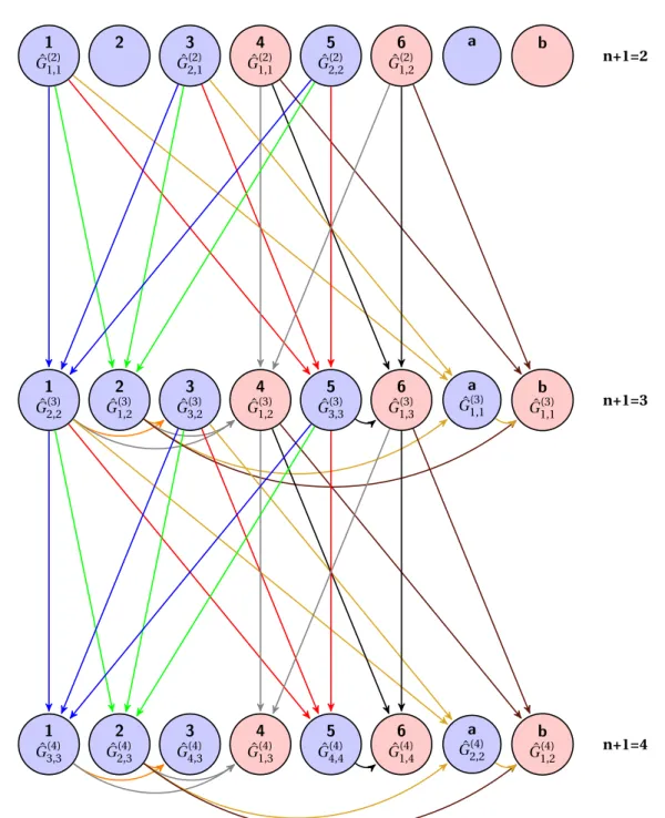
III.3 Modeling of a finite structure . . . 51
III.3.1 Layer-by-layer equation of motion . . . 51
III.3.1.i Few layer procedure . . . 53
III.3.1.ii Iterative procedure. . . 55
III.3.1.iii Effective hopping. . . 56
III.3.2 Layer-by-layer perturbation expansion . . . 57
III.3.2.i Nearest-layer hopping. . . 57
III.3.2.ii Second-nearest-layer hopping . . . 58
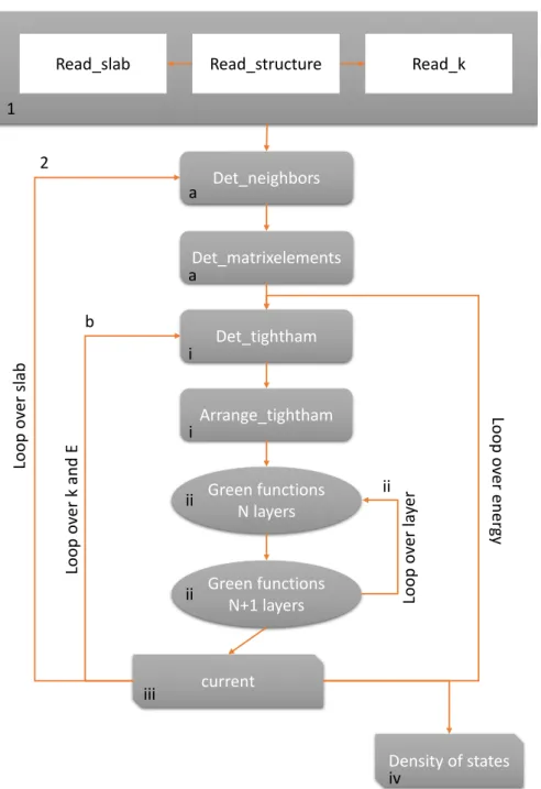
IV BEEM program 69 IV.1 Flow chart. . . 70
IV.2 Execution of the code and input files . . . 70
IV.2.1 Execution, input and output . . . 70
IV.2.2 Input files . . . 70
IV.2.2.i The main input-file structure.in (Listing IV.1) . . . 72
IV.2.2.ii The Hamiltonian input-file (Listing IV.2) . . . 72
IV.2.2.iii The k-point input-file . . . 74
IV.3 Building the hopping matrices and in-layer Hamiltonian . . . 75
IV.3.1 The tight binding matrix . . . 75
IV.3.2 The Hamiltonian matrix hban . . . 75
IV.3.3 Extracting the hopping matrices and the in-layer matrices from hban . . . 77
IV.4 Calculating the propagators and the current . . . 78
V Results and discussion 83 V.1 Tight-binding parametrization . . . 85
V.1.1 Papaconstantopoulos’ approach. . . 85
V.1.2 Harrison’s approach . . . 86
V.1.2.i Modified Harrison tight-binding parametrization 89 V.1.2.ii Silver band structure. . . 89
V.1.2.iii Multi-material parametrization . . . 90
V.2 Equilibrium evaluation of BEEM current . . . 91
V.2.1 2D projection of 3D Brillouin zones . . . 92
V.2.2 Gold: Au(001) and Au(111) . . . 94
V.2.3 Fe(001)/GaAs(001) . . . 95
V.2.4 Towards spintronics: Fe/Au/Fe/GaAs, the equilibrium ap-proach . . . 96
V.2.4.i Band structure (�k�) filtering . . . 98
V.2.4.ii Wave-function symmetry filtering . . . 98
V.3 Non-equilibrium approach . . . 100
V.3.1 Au(111). . . 101
V.3.1.i Surface density of states . . . 102
V.3.1.ii Effect of the damping parameter η . . . 102
V.3.1.iii Effect of the number of layers . . . 104
V.3.1.iv Effect of the parametrization . . . 106
V.3.1.v Au(111)/Si(111) and Au(111)/Si(001) . . . 106
V.3.2 Towards spintronics: preliminary results on Fe/Au/Fe spin-valve using the non-equilibrium approach. . . 108
V.3.3 Non-equilibrium calculation conclusion . . . 111
Contents ix
VI Conclusions and perspectives 115
A The formalism of the second quantization for fermions 119
A.1 Definition. . . 119
A.2 Anti-commutation rules . . . 120
A.3 Change of basis . . . 122
A.4 Second quantization Hamiltonian . . . 122
A.4.1 One body operator . . . 122
A.4.2 Two-body operator. . . 123
B Mathematical tricks 125 B.1 Fourier transform of a Green’s function . . . 125
B.2 Alternative derivation of Dyson equation for retarded and advanced Green functions . . . 126
B.3 Heisenberg’s equation of motion of the particle number operator ˆn 126 C Scientific production and resume 129 C.1 Collaboration. . . 129
C.2 Conferences . . . 129
C.3 Formations . . . 129
C.4 Teaching and popularization . . . 130
C.5 Articles . . . 130
C.6 Resume . . . 149
General introduction
S
PINTRONICS(contraction of spin and electronics) is a recent branch in the field of electronics where the spin of the electrons is exploited. Its official birth is 1988, after the discovery of the Giant Magneto-Resis-tance (GMR) by Albert Fert and Peter Gründberg [2,5]. Since 19971, it is used in our everyday life within the read-heads of the hard disk drive of our computers. The GMR effect consists in a significant diminution of the resistance in a thin film made of ferromagnetic and non-magnetic conductive layers, when an external magnetic field is applied. For instance, consider that at zero field, both magnetic layers have an anti-parallel magnetization. If we apply an external magnetic field in such a way that a reversal of the magnetization is induced and both magnetizations align, then, we observe that the resistance of the heterostructure drops drastically. It is due to the fact that the electrons, whose spin is not aligned with the magnetization of the metal where they propagate, experience more collisions than the ones whose spin is parallel to the magnetization of the metal. Such a system can be conceived as a spin polarizer/analyser: the first ferromagnetic slab polarizes the current and the second ferromagnetic slab analyzes the polarized current.It is interesting to notice that the advent of the spintronics could have taken place earlier with the discovery of the Tunneling Magneto-Resistance (TMR) by Jul-lière in 1975 [32]. The TMR is an effect similar to GMR which occurs in a magnetic tunnel junction, whose components consist of two ferromagnets separated by a thin insulator which replaces the non-magnetic spacer of GMR. However, at that time the discovery did not attract a lot of attention. The TMR was rediscovered in
the middle of the nineties [45,47]. Another ten years were needed to improve the
technique and to observe a TMR reaching several hundred percent at room tem-perature [30].
By coupling these GMR/TMR-structures with a semi-conductor, one can con-trol the spin-polarized current which is injected in the semi-conductor [46]. A cur-rent of electrons whose energy is winthin few eV above the Fermi level is injected from a transmitter within a metallic base which is in contact with a semi-conductor. If their energy is sufficient (these electrons are often called “hot electrons”, because their energy to overcome the Schottky barrier is much bigger than kBT ), they can
1The first use of spin-valve sensors in hard disk drive read heads was in the IBM Deskstar 16GP
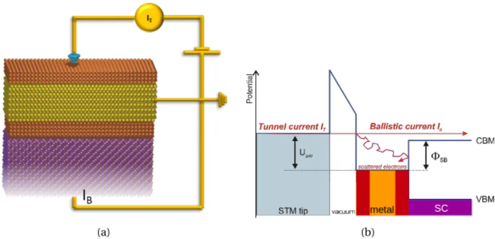
cross the Schottky Barrier at the metal/semi-conductor interface and be collected at the back of the semi-conductor. Such devices are the so-called “spin-valve” (see Fig.II.8, Chap.II).
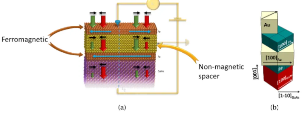
In this context, the Surfaces and Interfaces team of the Materials and Nano-sciences department of the Physical Institute of Rennes (IPR), in particular dr. Pas-cal Turban, has developed a Ballistic Electron Emission Microscope (BEEM). The principle of this microscope is presented in chapterIIand in figureII.1. It allows to image metal semi-conductor interfaces and to study structures that holds interest-ing features for the spintronics. In the last few years, several researchers from this team investigated the physical effects that govern the magneto-current by studying
a model structure Fe/Au/Fe/GaAs with BEEM experiments [26,25].
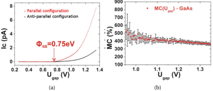
These experiments are quite long to carry out. Not only they require a long time to prepare the samples but each spectroscopy experiment takes several hours, and a few days are needed to obtain and analyze a spectrum like in Fig.II.3. For these reasons, a reliable theoretical model and a numerical code to quantify it can be very useful: they would help to target a system by making predictions and preselecting the sample to analyze.
The first model to describe a BEEM current, based on the free electron model, was proposed by Kaiser and Bell [34,4]. It was quite successful to predict the height of the Schottky barrier but it failed to explain the constant behavior of the current in some system, such as Au(111)/Si(001) and Au(111)/Si(111) [44], as described in chapterII. In 1996, F. J. Garcia-Vidal, P.L. de Andres and F. Flores [16] proposed a model, based on non-equilibrium approach by means of Keldysh formalism, where electrons propagate within the metal, by taking into account the band structure of the material in which they propagate. Their model was successful to explain the BEEM current behavior for Au(111)/Si(001) and Au(111)/Si(111), for both the inten-sity and the lateral resolution. However, in spite of its success about two decades ago, as it is based on the calculation of semi-infinite slabs, it cannot predict the behavior of electrons in extremely thin metallic films (few layer), or in heterostruc-tures like spin-valves, that are studied nowadays.
In this context, we have chosen to work again on the model of Garcia-Vidal, F. Flores and P. De Andres [16] and to extend it in order to describe finite structures. Our idea is:
1. to compare the non-equilibrium approach with a simpler equilibrium ap-proach. We ask ourselves if it is possible to interpret experimental results or to make predictions only by considering the band structure.
2. to provide a direct theoretical support to the experimentalists of our group by means of a user-friendly numerical code that can tell, for instance, what would happen if gold is replaced by silver in the Fe/Au/Fe/GaAs spinvalve, what would happen if we change the number of layers of iron etc. . .
In order to complete this program, we have decided to work with a tight-binding approach, as in the original work of F. Flores et al.. Of course, it would have been possible to use Green functions also within extended non-equilibrium Density Func-tional Theory calculations. However, for reasons detailed in sectionII.3.1, we be-lieve that tight-binding is the most appropriate method to fulfill our objectives.
This manuscript is organized in two parts: the first part is focused on the theo-retical and experimental background, and the second on the modeling of Ballistic Electron Emission Spectroscopy (BEES) on metallic films. Unlike the microscopy
General introduction 3 mode of the BEEM that allows to image buried structures, the spectroscopy mode
records the evolution of the BEEM current with respect to the applied bias, as de-scribed in chapterII. The first part of this thesis, the general background, corre-sponds to chaptersIandII, whereas chaptersIII,IVandV, together with the con-clusion, compose the second part where I derive and describe my results. In more details, in the first chapter of this thesis, some theoretical background, about equili-brium and non-equiliequili-brium perturbation-theory within second-quantization Green-functions is recalled. Although the reader who is already familiar with this formal-ism can skip this chapter, it might be useful, in order to get acquainted with the no-tation that is used in the next chapters. ChapterIIintroduces the Ballistic Electron Emission Microscopy and Spectroscopy. We shall see that the existing free-electron models failed to describe some experiments, like Au/Si, and that it is necessary to introduce a new model where the band structure of the material has to be taken
into account. In chapterIII, we extend the previous model of F. Flores and P. De
Andres’ group to thin films by avoiding their decimation technique through a dif-ferent layer-by-layer perturbation expansion. In this scheme we extend the older approach by considering second and third-nearest neighbor interactions.
Chap-terIVis devoted to the presentation of our new BEEM program. After presenting
the flow chart, we explain how to format an input file and what is the effect of the key parameters. Whereafter, we present some key subroutines that are required to
calculate the Green functions and hence the BEEM current. ChapterVpresents
our results obtained with this code and with the simpler equilibrium approach
de-scribed in chapterII. Finally, we draw our conclusions and some perspectives in
C
H
A
P
T
E
R
I
Theoretical background
A
S IT IS IMPORTANTto define a common language, and as thereare a lot of different notations in non-equilibrium Green func-tion formalism, a general background is presented in this chap-ter. We start with a quick overview of the second quantization and the derivation of the second-quantization Hamiltonian ; we then introduce Schrödinger, Heisen-berg and interaction pictures, and finally move to the fundamental principles of equilibrium and non-equilibrium perturbation theory using Green functions.
I.1 Introduction to second quantization
In the usual Schrödinger formalism of non-relativistic quantum-mechanic (it might improperly be called “first quantization”) the position x of the particle and its im-pulsion p are replaced by operators ˆX and ˆP acting on a Hilbert space (see for in-stance [15]). Commutation rules of these operators are established by analogy with Hamiltonian-mechanic formulation. Elements or vectors of the Hilbert space de-scribe possible configurations or states of a system with a fixed number N of par-ticles. The representation in the coordinate space of such a state is called a wave-function. This wave-function is a probability amplitude, that is to say a complex
function of the positions (x1,..., xN) and time t, ψ(x1,..., xN, t), whose square of
modulus is the probability density of finding the particles at points (x1,..., xN) and
time t. As well known, the wave-function is a solution of the Schrödinger equation, a partial differential equation in space and time.
This approach works well when we deal with a well-definite number of parti-cles. If, however, the interactions are such that the number of particles changes, a better procedure, called “second quantization” (the name might be misleading: there is no real quantization, it is just a formal tool), should be introduced. This second quantization formalism is fundamental in relativistic theories, where it was first formulated, because of particle creation and annihilation [13]. Yet, it turns out to be extremely important also in non-relativistic quantum-field theories [14,39] in several cases where the number of particles varies, like for Cooper pairs in super-conductivity. In our work, it is found to be extremely useful to describe the electron propagation from one metallic layer of the thin film to another, what can be seen intuitively as an electron annihilation and creation from the first layer to the sec-ond.
In order to describe such a process or, more generally, the transitions between states with different numbers of particles, the so-called creation and annihilation operators (or ladder operators) are introduced. Their role is fundamental in the formalism of second quantization. Though in the following we consider fermions, the simplest analogy to understand the physical meaning of ladder operators is in the boson case with the harmonic oscillator [9, chap. 5]. In quantum mechanics, the Hamiltonian operator for a one dimensional harmonic-oscillator is
H = Pˆx
2m+
1
2mω
2Xˆ2 (I.1)
where ˆX is the position operator and ˆPxis the x-component of the impulsion
op-erator of the particle. Since H is time independent, the quantum mechanical study of the harmonic oscillator reduces to the solution of the Schrödinger equation
H |ψ〉 = E |ψ〉 (I.2)
where E is the energy associated to an eigenstate |ψ〉 of the system. This is equiva-lent, in the x representation, to:
� −ħ 2 2m d2 dx2+ 1 2mω 2 x2 � ψ(x) = E ψ(x) (I.3)
The research of eigenvalues and eigenvectors of ˆH can be simplified by introducing the ladder operators (for bosons)
ˆ a =�1 2( ˆX + i ˆP ) (I.4) ˆ a†=�1 2( ˆX − i ˆP ) (I.5) with ˆX =�mωħ X and ˆP = � 1
mωħP . Because ˆX and ˆP obey the canonical
commu-tation relation [ ˆX , ˆP ] = i, the new operators obey
I.1. Introduction to second quantization 7 Another useful formula is
ˆ a†a =ˆ 1 2( ˆX − i ˆP )( ˆX + i ˆP ) =1 2( ˆX 2+ ˆ P2− 1) (I.7)
Comparing this equation with ˆH =ħω2 � ˆX2+ ˆP2� we see that ˆ
H = ˆa†a +ˆ 1 2 =a ˆˆa†−1
2 (I.8)
So that the eigenvectors of the particle-number operator ˆn = ˆa†a are eigenvectorsˆ of ˆH . It is then possible to replace ˆH by ˆn in the Schrödinger equation
ˆ
n |v〉 = v |v〉 (I.9)
The eigenvalues of the quantum harmonic oscillator are thus Ev=ħω � v +1 2 � (I.10) It is possible to find the eigenvalues of ˆn by using commutation relations:
[ ˆn, ˆa] = − ˆa (I.11) [ ˆn, ˆa†] = ˆa† (I.12) which gives [ ˆn, ˆa] |v〉 = ˆn( ˆa |v〉) − v( ˆa |v〉) = − ˆa |v〉 (I.13) ˆ n ˆa |v〉 = (v − 1) ˆa |v〉 (I.14)
in other words, ( ˆa |v〉) is eigenvector of ˆn with eigenvalue (v − 1). This means that ˆ
a acts on |v〉 to produce, up to a multiplicative constant, the state |v − 1〉. A similar equations holds for ˆa†
ˆ
n ˆa†|v〉 = (v + 1) ˆa†|v〉 (I.15)
This times, ˆa†acts on |v〉 to produce, up to a multiplicative constant, |v + 1〉. For this reason, ˆa is called a lowering operator and ˆa† a raising operator. They lower or raise the energy of a quantity ħω. In quantum field theory, these operators are respectively called "annihilation" and "creation" operators because they destroy and create particles, which correspond to our quantum of energy. There is however a complete analogy between the two cases.
The fermion case, though conceptually identical, brings in more cumbersome algebra, because of the antisymmetrization requirements of the N-particle
wave-function. For this reason, we placed the general treatment in the appendixA. We
just remind that the Hilbert space on which these operators act is what is known as a Fock space, that is to say, a stack of infinite Hilbert-spaces communicating through fields and operators and comprising the vacuum, a-zero particle space, a one-particle space, a two-particles space, etc . . . In what follows we describe the second quantization Hamiltonian as we shall use in our work.
I.1.1 Second quantization Hamiltonian
The Hamiltonian of a system of N interacting-electrons evolving within a periodic potential U (�ri) can be written as
ˆ H = N � i =1 � −ħ2 2mΔi+U (�ri) � � �� �
monoelectronic Hamiltonian sum h(�ri)
+1 2 � i , j (i �=j ) V (�ri−�rj) � �� � two-body term (I.16)
where U (�ri) = −e�ku(�ri− �Rk) is the interaction with the nuclei and V (�ri−�rj) =
e2/(4π�0|�ri−�rj|) is the Coulomb repulsion. As shown in the appendixA, it can be
rewritten in second quantization as ˆ H =� k,l 〈k |h |l〉 ˆc†kˆcl+ 1 2 � k,l ,m,n 〈kl |V |mn〉 ˆck†ˆc † l ˆcnˆcm =� k,l Tklˆck†ˆcl+ 1 2 � k,l ,m,n Vkl nmˆck†ˆcl†ˆcnˆcm (I.17)
where {〈�r|l〉 = ϕl(�r)} is a complete basis for the wave-function (l including spin)
and where ˆ Tkl=〈k |h(�r)|l〉 =� k � k � � � � − ħ2 2mΔk+U (�rk) � � � �l � � �� � ε0δk,l +� i �=k 〈k |U (�ri)|l〉 � �� � −tkl = � d3�r ϕ∗k(�r) h(�r) ϕl(�r) (I.18) and Vkl nm=〈ϕk⊗ ϕl|V |ϕm⊗ ϕn〉 = � d3�r � d3�r�ϕ∗k(�r)ϕ∗ l(�r�) V (�r −�r�) ϕm(�r)ϕn(�r�) (I.19)
The final Hamiltonian can be therefore written as: ˆ H =� k,l [ε0δk,l− tkl] ˆck†ˆcl+ 1 2 � k,l ,m,n Vkl nmˆc†kˆcl†ˆcmˆcn (I.20)
I.1.1.i Tight-binding model
The tight-binding model consists in making the assumption that the Coulomb in-teraction of the electrons is negligible compared to their kinetic and lattice ener-gies. In other words, Vkl nm=0 in Eq. (I.20). The Hamiltonian is then reduced to
ˆ Ht b=
�
k,l
[ε0δk,l− tkl] ˆc†kˆcl (I.21)
The physical interpretation of the terms is the following: ε0 corresponds to the
atomic energy or to the orbital energies in the case of multi-orbital atoms (as in the following of this work). It is the on-site energy. The so-called hopping term tk,lˆck†ˆcl
I.2. Pictures 9
with quantum number k with an amplitude tk,l. The tight-binding model has been
very used in the literature because it allows reproducing electron structure with lo-calized orbitals (i.e., only neighbor interactions are taken into account) of many materials or to model electronic transport, as we shall see below, and has the ad-vantage that it can be extended in a straightforward manner to describe problems where the electron correlation is not negligible, as done, for instance in the Hub-bard model [27,28,29].
I.1.1.ii Hubbard model
In his approach, Hubbard supposed that the most important part of the electron-electron interaction is due to the on-site Coulomb repulsion [27,28,29]. In other words, Vkl nm�= 0 only when k, l, n and m all refer to the same site (say, site �Ri). In
that case by writing the spin explicitly, the Coulomb repulsion is Viσi σ�,i σi σ�= e 2 4πε0 � d3�rd3�r���ϕiσ(�r) � �2� 1 ��r −�r��� � �ϕiσ�(�r�)��2 (I.22)
and the Hamiltonian writes ˆ H = ˆHt b+ ˆHU =� k,l [ε0δk,l− tkl] ˆck†ˆcl+U � i ,σ ˆ niσnˆi ¯σ (I.23)
where U = Viσi σ�,i σi σ�/2 and where ˆniσ=ˆci†σˆciσis the number of particle operator
of spin σ at site |�R〉i. In general, ˆc†iˆciis the number of particle operator in the state
at site �Ri. In the case of, e.g., transition metals, characterized by more than one
orbital per site, Eq. (I.23) should be generalized in order to take into account of the extra degree of freedom [28].
I.2 Pictures
In the next chapters, we want to describe Ballistic Electron Emission Microscopy that is a technique based on the Scanning Tunneling Microscope. In this microscopy, the electric field induced by the STM tip can be seen as a weak external perturba-tion. Hence it seems natural to use a perturbation approach. In this subsection the various representations, or pictures, of quantum mechanics are recalled, namely, Schrödinger, Heisenberg and interaction pictures. As the name suggests, the in-teraction picture is the natural framework to formulated the perturbation theory, Schrödinger and Heisenberg pictures are a necessary complement to understand it.
I.2.1 Schrödinger and Heisenberg pictures
In the Schrödinger picture, only the wave-functions are time dependent, while in the Heisenberg picture it is the operators that hold the time dependence. While the wave-functions in the Schrödinger picture obey the usual Schrödinger equa-tion (I.29) below, the operators in the Heisenberg representation obey the
Heisen-berg equation of motion, through the commutator with ˆH :
By definition, for all values of t, the expectation value of an operator is the same in both representations: � ψS(t) � � ˆOS � �ψS(t) � =�ψH � � ˆOH(t) � �ψH � (I.25) Where label S refers to the Schrödinger representation and label H to the Heisen-berg representation. In order to simplify the calculation, let’s take t = 0 the time where both representations coincide:
ˆ OH(t = 0) = ˆOS (I.26) � �ψS(t = 0) � =��ψH � (I.27) It is useful at this point to introduce the evolution operator ˆU (t , t0) as the operator
that leads from the state |ψS(t0)〉 to the state |ψS(t)〉:
� �ψS(t)
�
= ˆU (t , t0)��ψS(t0)� (I.28)
Of course, this operator must be related to the Hamiltonian, because for time de-pendent phenomena, the Hamiltonian can be seen as the infinitesimal generator of time translations, i.e., it leads from the state |ψ(t)〉 to the state |ψ(t + dt)〉. This is a consequence of the Schrödinger equation for a time dependent Hamiltonian:
iħ∂ ∂t � �ψS(t) � = ˆH (t )��ψS(t) � (I.29) Because of the hermiticity of ˆH the time derivative∂t
� ψS(t) � �ψS(t) � =0, i.e., the probability is conserved.
All this, implies that: ˆU (t , t0) is a unitary operator: which obeys the following
identities:
ˆ
U (t0, t0) = l1 (I.30)
and because of the conservation of probability ˆ
U†(t, t0) ˆU (t , t0) = l1 (I.31)
So that:
ˆ
U−1(t, t0) = ˆU†(t, t0) (I.32)
Furthermore, if the time-reversal invariance can be used, we also have ˆ
U−1(t, t0) = ˆU†(t, t0) = ˆU (t0, t) (I.33)
as
ˆ
U (t0, t) ˆU (t , t0) = l1 (I.34)
Using the expression for the time dependent wave-function and the equality (I.25), we can move from Schrödinger to Heisenberg representations using the evo-lution operator as follows:
ˆ
OH(t) = ˆU†(t,0) ˆOSU (t , 0)ˆ (I.35)
This allows to find out the explicit expression of the evolution operator in terms of the Hamiltonian. In fact, one recovers the usual results for time-independent
I.2. Pictures 11 Hamiltonians by noting that in this case, the solution of Schrödinger equation for
the evolution operator is ˆ
U (t , t0) = e−i ˆH (t −t0)/ħ (I.36)
whose general integral form is ˆ U (t , t0) = ˆT � exp � −i �t t0 dt�H (tˆ �) �� (I.37)
where ˆT is the time-ordering operator. It orders time dependent operators from
right to left in ascending time and adds a factor (−1)p where p is the number of
permutation of fermion operators. As we shall see in sections, it is a key operator for the definition of Green functions.
I.2.2 Interaction picture
As said above, the interaction picture is the best representation for perturbation theory, i.e. when the Hamiltonian is written as ˆH = ˆH0+ ˆV and it is supposed
that we can solve the Schrödinger equation for a time-independent ˆH0(but not
for ˆH ) and that ˆV is a “small” perturbation of ˆH0. It is an intermediate
representa-tion, between Schrödinger and Heisenberg ones, introduced by Dirac (sometimes it is called Dirac representation). In this representation, both operators and wave-functions evolve in time. The wave-wave-functions however develop under the influence of the “difficult” interaction part of the Hamiltonian
ˆ
H = ˆH0+ ˆV (I.38)
where ˆH0is time independent as stated above. In this framework, the time-evolution
operator ˆUI(t,0) is given by
ˆ
U (t , 0) = e−i ˆH0t /ħUˆI(t,0) (I.39)
ˆ
U (0, t ) = ˆUI(0, t)ei ˆH0t /ħ (I.40)
This operator has the same unitary property that an ordinary time evolution oper-ator. So it is possible to write:
ˆ
U (t , t0) = e−i ˆH0t /ħUˆI(t, t0)ei ˆH0t0/ħ (I.41)
Again, at t = 0 all the representations coincide. The reason to define the time evo-lution operator in this way is that, for a small perturbation ˆV , ˆUI(t, t0) is close to
unity, that is ˆUIencloses the “smallness” of the perturbation ˆV .
Using again the equality |ψS(0)〉 = |ψH〉 = |ψI(0)〉 and Eq. (I.39), the matrix
ele-ments are: � ψH � � ˆOH(t) � �ψH � =�ψS(t = 0) � � ˆOS � �ψS(t = 0) � =�ψS(t = 0) � � �Uˆ†(t,0) ˆOSU (0, t )ˆ � � � ψS(t = 0) � = � ψH � � �UˆI†(t,0)e i ˆH0t /ħOˆSe−i ˆH0t /ħUˆI(t,0)�� � ψH � =�ψI(0) � � �UˆI†(t,0) ˆOI(t) ˆUI(t,0) � � � ψI(0) � (I.42)
This important result can be interpreted as the fact that the operators in the inter-action picture evolve with the H0part, that we are supposed to know:
ˆ
OI(t) = ei ˆH0t0/ħOˆSe−i ˆH0t /ħ (I.43)
while the wave-functions obey �
�ψI(t)�= ˆUI(t,0)
�
�ψS� (I.44)
That is, the unknown part (but supposed small). We shall see in the next section how to get a closed solution for this problem, at least for a tight-binding Hamilto-nian, by means of a Green function approach.
I.3 Green functions
This section introduces the concept of Green functions within the second quan-tization formalism of quantum mechanics. They are also called propagators, as they describe the propagation of an excitation from (x, t) to (x�, t�). We remind that
the Green function method is very useful and widely employed independently of quantum mechanics in the theory of ordinary and partial-differential equations like Poisson equation or Maxwell equations in electrodynamics (see, eg, [31]). In this case, Green functions are used to re-express differential equations as integral equations, to be solved, eventually, by perturbation methods. Mutatis mutandis, this method has been used in quantum mechanics to solve the Schrödinger equa-tion in its second-quantizaequa-tion form, as detailed below. In this case, the single-particle Green function allows to find the expectation value of any single-single-particle operator in the ground state, the ground-state energy and the excitation spectrum of the system [14, Chap. 3]. Green functions are also particularly useful for prob-lems solved by means of perturbation theory as they can be represented diagram-matically through Feynman diagrams [38].
The reason why we introduce the Green-function formalism in our work is that the electric current can be expressed in a straightforward way through this formal-ism, as we shall see in sectionIII.1.
I.3.1 Definition
The single-particle Green function is defined in Heisenberg representation by i ˆGi jσ(t, t�) = � ΨH0 � � �Tˆ � ˆciσ(t) ˆc†jσ(t�) � � � � ΨH0 � � ΨH0��Ψ0H� (I.45) where |ΨH
0〉 is the Heisenberg ground state of the interacting system satisfying
ˆ
H |ΨH0〉 = E |ΨH0〉 (I.46)
with the second quantification Hamiltonian of Eq. (I.20). We suppose from now
on that it is normalized (〈ΨH
0|ΨH0〉 = 1) and remove the denominator in Eq. (I.45).
Here, the annihilation ˆciσ(t) is a Heisenberg operator with the time dependence
I.3. Green functions 13
i and j label the components of the field operator. The product ˆT represents a
generalization of ˆ T�ˆciσ(t) ˆc†jσ(t�) � = � ˆciσ(t) ˆc†jσ(t�) t > t� ±ˆc†jσ(t�) ˆciσ(t) t < t� (I.48) where the ± sign refers to bosons/fermions. That’s why this product is called time ordering: operators are ordered from right to left in ascending time order and a
factor (−1)p is added for p interchanges of fermion operators, from the original
order. From (I.46) and (I.47) we can write i ˆGi jσ(t, t�) = eiE0N(t−t�)/ħ � Ψ0H � � � ˆcie−i ˆH (t −t �)/ħ ˆc†j�� � Ψ0H � t > t� ±e−iE0N(t−t�)/ħ � ΨH 0 � � � ˆc†jei ˆH (t −t �)/ħ ˆci � � � Ψ0H � t�>t (I.49)
The factor eiE0N(t−t�)/ħis merely a complex number which can be taken out of matrix element. In contrast, the operator ˆH must remain between the field operators.
I.3.2 Retarded and advanced Green functions
A very interesting representation of the propagator is the Lehmann representation where the Green function is expressed in frequency space because information about the excitation spectrum can be extracted in a natural way. For this purpose, we re-write Eq. (I.45) in the form (still in Heisenberg picture):
i ˆGi jσ(t, t�) = −eiE0N(t−t�)/ħ�n � ψ(N )0 � � � ˆcie−i ˆH (t −t �)/ħ�� � ψ(N +1)n � � ψ(N +1)n � � � ˆc†j � � � ψ(N )0 � t > 0 e−iEN 0(t−t�)/ħ�n � ψ(N )0 �� � ˆc†jei ˆH (t −t �)/ħ�� � ψ(N −1)m � � ψ(N −1)m � � � ˆci � � � ψ(N )0 � t < 0 (I.50) The�� �ψ(N −1)m � and�� �ψ(N +1)n �
denote a complete set of eigenstates of the (N − 1) and (N + 1) electron systems, respectively, characterized by the quantum numbers m
and n. Their corresponding energies are EN −1
m and EnN +1, while E0N is the
ground-state energy of the N -electron system. Since the volume of the system is kept con-stant, the change in energy
An=EN +1n − E0N (I.51)
is the electron affinity. The other difference
Im=EmN −1− E0N (I.52)
is the ionization potential. Introducing these quantities in Eq. (I.50), it gives i ˆGi jσ(t, t�) = − eiAn(t−t�)/ħ� n � ψ(N )0 �� � ˆci � � � ψ(N +1)n � � ψ(N +1)n � � � ˆc†j � � � ψ(N )0 � t > 0 e−iIm(t−t�)/ħ� n � ψ(N )0 � � � ˆc†j � � � ψ(N −1)m � � ψ(N −1)m � � � ˆci � � � ψ(N )0 � t < 0 (I.53) Using the Fourier transform of the Green function
ˆ Gi j(t) = 1 2π �+∞ −∞ ˆ Gi j(ω)e−iω(t−t �) dω (I.54)
Eq. (I.53) becomes (see, for example [14]): ˆ Gi j(ω) = � n αi(n)α†j(n) ħω − An+iη +� m βi(m)β†j(m) ħω − Im− iη (I.55) where αi(n) = 〈ψ(N )0 |ˆci|ψ(N +1)n 〉 and β†j(n) = 〈ψ (N ) 0 |ˆc†j|ψ(N −1)m 〉. η is a positive
in-finitesimal quantity which ensures the correct analytic properties of ˆGi , j(ω). We
can introduce the chemical potential by rewriting Eq.I.51
EnN +1− E0N=EnN +1− E0N +1+E0N +1− E0N
=εN +1n + µ (I.56)
and in the case of a macroscopic body, as there is a large number of electrons we can write
µ = EN +1n − E0N� EmN −1− E0N (I.57)
Thus, Eq. (I.55) becomes ˆ Gi j(ω) = � n αi(n)α†j(n) ħω − µ − εN +1n +iη +� m βi(m)β†j(m) ħω − µ + εN +1n − iη (I.58) From this last equation we can introduce two new Green functions, the so-called retarded and advanced Green functions which are defined, in the Lehman repre-sentation, by (see [14, Sec. 7]):
ˆ Gi jR(ω) =� n αi(n)α†j(n) ħω − µ − εN +1n +iη +� m βi(m)β†j(m) ħω − µ + εN +1n +iη (I.59) ˆ Gi jA(ω) =� n αi(n)α†j(n) ħω − µ − εN +1n − iη +� m βi(m)β†j(m) ħω − µ + εN +1n − iη (I.60) The corresponding time-dependent Green functions are (see [14]):
ˆ GRi , j(t − t�) = −iθ(t − t�)�ψ 0 � � � � ˆci(t), ˆc†j(t�) � � � � ψ0 � (I.61) ˆ Gi , jA (t − t�) = iθ(t�− t)�ψ 0 � � � � ˆci(t), ˆc†j(t�) � � � � ψ0 � (I.62)
where the curly bracket denotes an anti-commutator and θ(t − t�) the Heaviside
function. The retarded Green function is also called a propagator since it gives the wave-function at any time as long as the initial condition is given.
As said above, those Green functions gives access to spectral quantities, such as the density of states
ρ(ε) =� n δ(ε − E n) =−1 πImTr ˆG R(ε) (I.63) The quantity ρi(ε) = − 1 πIm ˆG R i ,i(ε) (I.64)
is the local density of states. It is a relevant quantity in particular when there is no translational invariance. That is what is measured by scanning tunneling micro-scopes.
I.3. Green functions 15
Figure I.1: Starting from t = −∞, the perturbation is adiabatically switch-on until t = 0, time at which the system is described by the full Hamiltonian H . Then the perturbation is adiabatically switch-off until t = +∞, and the system go back in its original state |ψ0〉
I.3.3 Perturbation expansion
The aim of the perturbation expansion is to generate exact eigenstates of the inter-acting system, described by ˆH , from the eigenstates of the non-interacting system, described by ˆH0, as we suppose to know all about the latter, and from the
pertur-bation ˆV . In other words, we want to express the Green function of the interacting system i ˆGi jσ(t − t�) = � ψH0 � � �Tˆ � ˆciσ(t) ˆc†jσ(t�) � � � � ψH0 �
in terms of Green functions of the non-interacting system and ˆV . In order to do that we rewrite the full Hamiltonian ˆH = ˆH0+ ˆV and introduce a new time dependent Hamiltonian:
ˆ
H (t ) = ˆH0+e−�|t|Vˆ (I.65)
where � is a small quantity which allows to switch-on and switch-off the pertur-bation adiabatically, that is very slowly.1 At very large times, both in the past and in the future, the Hamiltonian reduces to ˆH0. At time t = 0, ˆH describes the full
interacting-system. This is described in Fig.I.1. If the process is slow enough, then any result is independent of � (adiabatic theorem [43, Chap. 17, Sec. II.8]).
As we are interested in a time dependent problem that depends on the small quantity �, we shall use the interaction picture (Eq.I.44):
|ψI(t)〉 = ˆU�(t, t0)|ψI(t0)〉 (I.66)
In the limit t0→ −∞, the Schrödinger-picture state reduces to:
�
�ψS(t0)�=e−iE0t0/ħ��φ0� (I.67)
where��φ0� is a time-independent eigenstate of the unperturbed Hamiltonian ˆH0
with eigenvalue E0. Moreover, as said above, at time t = 0 all three pictures
coin-cide. Then � �ψH � =��ψI(t = 0) � = ˆU�(0,−∞) � �φ0� (I.68)
1It should be reminded that originally an adiabatic transformation refers to a thermodynamic
trans-formation with no heat exchange. Roughly speaking, the slow temporal evolution is supposed to keep the state evolution from ˆH0to ˆH in a one-to-one correspondence that should mimic an adiabatic trans-formation.
This last equation is a very important result as it expresses an exact eigenstate of the interacting system in terms of an eigenstate of the non-interacting one.
Coming back to the definition (I.45) and using the integral form (I.37), we have: � ψ0H � � �Tˆ � ˆciσ(t) ˆc†jσ(t�) � � � � ψH0 � = ∞ � n=0 (−i)n n! � dt1... � dtn � φ0 � � �Tˆ� ˆV(t1)... ˆV (tn) ˆciσ(t) ˆc†jσ(t�) � � � � φ0 � (I.69) for � → 0. This equation could seem quite complicated due to the time-ordering operator.2However, G. C. Wick has built a theorem [58] which allows to write down such time ordering product by pair, if there are the same number of creation and annihilation operator. Here, as our Hamiltonian is quadratic, we can use this pow-erful theorem. The proof of it is quite tedious and can be found, for example, in Ref. [14, Sec. 8]. Here, we will just see how we can use it:
n = 0: ˆ T� ˆV(t1)... ˆV (tn) ˆciσ(t) ˆc†jσ(t�) � = ˆT�ˆciσ(t) ˆc†jσ(t�) � =gˆi jσ(0) n = 1: ˆ T� ˆV(t1)... ˆV (tn) ˆciσ(t) ˆc†jσ(t�) � = ˆT� ˆV(t1) ˆciσ(t) ˆc†jσ(t�) � = ˆT�ˆciσ(t) ˆc†jσ(t�)� ˆV(t1) ˆT � ˆciσ(t) ˆc†jσ(t�) � =gˆ(0)i jσV ˆˆgi jσ(0) n = 2: ˆ T� ˆV(t1) ˆV (t2) ˆciσ(t) ˆc†jσ(t�) � = ˆT�ˆciσ(t) ˆc†jσ(t�)� ˆV(t1) ˆT � ˆciσ(t) ˆc†jσ(t�)� ˆV(t1) ˆT � ˆciσ(t) ˆc†jσ(t�) � =gˆi j(0)σV ˆˆgi jσ(0)V ˆˆg(0)i jσ
Iterating up to infinity we obtain Dyson’s equationI.70that links the full Green
function (perturbed) with the unperturbed one and with the perturbation ˆV in the
following form ˆ Gi jσ=gˆi jσ(0) +gˆi jσ(0)V ˆˆgi j(0)σ+gˆi jσ(0)V ˆˆgi jσ(0)V ˆˆgi j(0)σ+... =gˆi jσ(0) +gˆi jσ(0)V ˆˆGi jσ =�1 − ˆg(0) i jσV �−1 ˆ g(0)i jσ (I.70)
whose integral form is ˆ
Gi jσ(t1,t1�) = ˆgi j(0)σ(t1, t1�) +
�
d4t2d4t3gˆi j(0)σ(t1, t2) ˆV (t2, t3) ˆGi jσ(t3, t1�) (I.71)
2We have even oversimplified it (see [14]), as we have assumed that the normalization of 〈ψH 0|ψ0H〉 =
1 implies that of |φ0〉 and this is not generally true. Actually the denominator of Eq.I.45should also be expanded in the interaction representation, leading to the elimination of the so-called non-connected diagrams of Eq.I.69. In what follows, we suppose it to be done already.
I.3. Green functions 17 There is a formally simpler approach to derive Dyson equation whose
simplic-ity however hides some important features that we shall use in sectionI.4. This
approach is shown in AppendixB.2.
The Dyson equation is particularly useful because even if we cannot invert the large matrix ˆH to compute ˆGR, we have re-expressed it in term of the unperturbed Green function ˆgi jσ(0) and the perturbation ˆV that are usually easier to evaluate.
In practice, if we want to know the propagator at a given order, we just stop the above expansion at this order. However, this could lead to misleading results. Moreover, we should be sure that the seriesI.70converges, which is not always the case, depending on the perturbation.
We have seen that this formalism is based on the fact that the perturbation is time independent. However, if it is not the case, then, one has to use another the-ory called non-equilibrium perturbation thethe-ory based on non-equilibrium Green-function (NEGF), or Keldysh Green Green-function, as explained in Sec.I.4.
I.3.4 Resolution through equation of motion
The Green functions can be also obtained by solving an equation of motion without using the time evolution operator, thereby, avoiding to pass through the interaction
picture. This can present some advantages, as we shall see in Chap.III. We start
with the time derivative of Heisenberg operators of the Green function: iħ∂tGˆi jσ(t − t�) = � ∂tTˆ � ˆciσ(t) ˆc†jσ(t�) �� +� ˆT��∂tˆciσ(t)� ˆc†jσ(t�) �� (I.72) As the time-ordering operator ˆT can be represented by the step function
θ(t − t�) ˆciσ(t) ˆc†jσ(t�) for t > t� (I.73)
θ(t�− t) ˆc†jσ(t�) ˆc
iσ(t) for t�>t (I.74)
its time derivative is given by a dirac δ-function and one obtains: iħ∂tGˆi jσ(t − t�) = � ∂ ∂tθ(t − t �) � ˆciσ(t) ˆc†jσ(t�) − � ∂ ∂tθ(t �− t) � ˆc†jσ(t�) ˆc iσ(t) +� ˆT��∂tˆciσ(t)� ˆc†jσ(t�) �� =δ(t − t�) � ˆciσ(t) ˆc†jσ(t�) + ˆc†jσ(t�) ˆciσ(t) � � �� � � ˆciσ, ˆc†jσ� � =δi jδσσ� + � ˆ T�∂tˆciσ(t) � �� � =1
iħ� ˆciσ, H� cf. Eq. (I.24)
ˆc†jσ(t�)�
�
(I.75) The time derivative of the Heisenberg operator ˆciσ(t) is obtained through Eq. (I.24).
Consider a simple tight binding Hamiltonian ˆ
H =�
i j
ti jˆci†ˆcj with ti i=ε(i ) (I.76)
Using Eq. (B.22), the commutator� ˆciσ, ˆH� writes
[ ˆciσ, ˆH0] = � ˆciσ, ˆc†lσˆcmσ � =� l m δi lˆcmσtl m = � m ti mˆcmσ , (I.77)
Finally, the equation of motion is
iħ∂tGˆi jσ(t − t�) = δ(t − t�)δi j+�mti mGˆm jσ(t − t�) (I.78)
As we are interested by the energy spectrum, we have to use the Fourier transform in time domain of the Green function:
ˆ Gi jσ(ω) = �+∞ −∞ ˆ Gi jσ(t)eiω(t−t �) dt ˆ Gi jσ(t) = 1 2π �+∞ −∞ ˆ Gi jσ(ω)e−iω(t−t �) dω (I.79)
whose time derivative is
iħ∂tGˆi jσ(t) =iħ 2π �+∞ −∞ −i ω ˆ Gi jσ(ω)e−iω(t−t �) dω =ħω 2π �+∞ −∞ ˆ Gi jσ(ω)e−iω(t−t �) dω (I.80)
And, the Fourier transform of Dirac delta function is δ(t − t�) = �+∞ −∞ dω 2πe−iω(t−t �) (I.81) Hence, the Fourier transform of Eq. (I.78) is
�+∞ −∞
dω
2πiħ∂t� ˆGi jσ(ω)e−iω(t−t
�)� = δi j �+∞ −∞ dω 2πe−iω(t−t �) +� m ti m �+∞ −∞ dω 2πGˆm jσ(ω)e−iω(t−t �) (I.82) Factorizing and regrouping:
1 2π �+∞ −∞ dω e−iω(t−t�)� ħω ˆGi jσ(ω) − δi j− � m ti mGˆm jσ(ω) � =0 (I.83)
That implies, because of the completeness of the complex-exponential basis: ħω ˆGi jσ(ω) = δi j+
�
m
ti mGˆm jσ(ω) (I.84)
If the system is infinite, we can also use the Fourier-transform of the Green func-tions and the hopping matrices in space domain in order to diagonalize Eq. (I.84). In this case, we would obtain:
ħω ˆG�kσ(ω) = 1 + t�kGˆ�kσ(ω) �
ħω − t�k� ˆG�kσ(ω) = 1 (I.85)
where t�k≡N1
�
i , jti , jei�k·(�Ri−�Rj). In the case of metal thin-films, we lose the full 3D
periodicity, so we shall not perform the Fourier transform in one of the three direc-tions. Therefore we have to solve directly the equation systemI.84, as shown in the
I.4. Non-equilibrium perturbation-theory and Green functions 19
Figure I.2: Contour C. The upper branch is called “positive branch” and the lower “negative branch”. The ± notation follows [11] which is the same as Lifshitz nota-tions [38], except that the positive and negative branches are exchanged. See Ta-bleI.1for a summary of the different notations.
I.4 Non-equilibrium perturbation-theory and Green functions
In non-equilibrium problem, there is no guarantee that the system returns to its initial state at asymptotically large times: this is a fundamental condition tode-velop perturbation theory as we have seen in sec.I.3.3. Therefore, perturbation
theory cannot be applied along the same lines: any references to asymptotically large times should be avoided in the non-equilibrium theory. This implies, as we shall see below, that a different approach has to be looked for in the adiabatic in-troduction of the perturbation. Such an approach leads to a new contour for time integration, but, in spite of some conceptual complications, several formal aspects of non-equilibrium perturbation theory (like Dyson’s equation) keep an equivalent structure as in equilibrium theory.
The non-equilibrium is formulated as follows. We consider a system evolving under the Hamiltonian
ˆ
H (t ) = ˆh + ˆH�(t) (I.86)
where h is the time independent part of the Hamiltonian, and it can be split in two parts: ˆh = ˆH0+ ˆHi, where ˆH0is “simple” (it can be diagonalized, and hence, Wick’s
theorem applies) and ˆHi may contain the many body aspects of the problem, and
hence requires a special treatment. ˆH�(t) is the external time-dependent perturba-tion.
I.4.1 Contour-ordered operator
As shown in sectionI.2.1a general operator in Heisenberg picture can be written in terms of interaction-picture operators:
ˆ
OH(t) = ˆUh†(t, t0) ˆOh(t) ˆUh(t, t0) (I.87)
with the unitary operator ˆUh(t, t0) that determines the state vector at time t in
terms of the state vector at time t0:
ˆ Uh(t, t0) = ˆT � exp � −i �t t0 dt�Hˆ� h(t�) �� (I.88)
ˆ
T is the time ordering operator which arranges the latest times to left. ˆHh�(t) is the interaction picture of ˆH�(t)
ˆ
Hh�(t) = eih(t−t0)Hˆ�(t)e−ih(t−t0) (I.89)
The following property ˆUh(t0, t) = ˆUh†(t, t0) of the evolution operator, allows to
rewrite equation (I.87) with a contour-ordered operator as follows: ˆ OHˆ(t) = ˆTC � exp � −i � Cdτ ˆH � h(τ) � ˆ Oh(t) � (I.90) Where the contour C is represented in Fig.I.2.
The proof of equivalence Eq. (I.87) and Eq. (I.90) is done by: ˆ TC � exp � −i � Cdτ ˆH � h(τ) � ˆ Oh(t) � = ∞ � n=0 (−i)n n! � Cdτ1... � Cdτn ˆ TC� ˆHh�(τ1)... ˆHh�(τn) ˆOh(t) � (I.91) Divide the contour in two branches
� C = � → + � ← (I.92)
where�→ goes from −∞ to +∞ and�←from +∞ to −∞. Replacing
con-tour integral by this sum generates 2n terms. For the demonstration, let’s
consider one of them: � → dτ1 � → dτ2 � ← dτ3... � ← dτnTˆC� ˆHh�(τ1)... ˆHh�(τn) ˆOh(t) � = � ← dτ3... � ← dτnTˆ←� ˆHh�(τ3)... ˆHh�(τn) ˆOh(t) � × � → dτ1 � → dτ2Tˆ←� ˆHh�(τ1) ˆHh�(τ2) � (I.93)
There are�mn�=n!/[m!(n − m)!] combinations of m integrals from −∞ to
+∞ (in the above example m = 2) amongst the 2n terms generated terms.
All these terms give the same contribution. Thus we can write � Cdτ1... � Cdτn ˆ TC� ˆHh�(τ1)... ˆHh�(τn) ˆOh(t) � = ∞ � n=0 n! m!(n − m)!× � ←dτm+1... � ←dτn ˆ T←� ˆHh�(τm+1)... ˆHh�(τn) ˆOh(t) � × � → dτ1... � → dτmTˆ←� ˆHh�(τ1)... ˆHh�(τm) � (I.94)
I.4. Non-equilibrium perturbation-theory and Green functions 21
Replacing n − m = k, both k and m can be summed from 0 to ∞ as long as their sum equals n. This is achieved by inserting a Kronecker delta:
∞ � m,k=0 n! m!k!δn,k+m �� ← dτ1... � ← dτkTˆ←� ˆHh�(τ1)... ˆHh�(τk) �� ˆ Oh(t) × �� → dτ1... � → dτmTˆ→� ˆHh�(τ1)... ˆHh�(τm) �� (I.95) Going back to eq. ((I.91)), the n-sum is (due to the factor δn,k+mand
simpli-fying the n! terms): ˆ TC � exp � −i � Cdτ ˆH � h(τ) � ˆ Oh(t) � = ∞ � k=0 (−i)k k! � ←dτ1... � ←dτk ˆ T←� ˆHh�(τ1)... ˆHh�(τk)� ˆOh(t) × ∞ � m=0 (−i)m m! � → dτ1... � → dτmTˆ→� ˆHh�(τ1)... ˆHh�(τm)� ˆOh(t) (I.96)
The factors multiplying ˆOh(t) are ˆU†(t, t0) and ˆU (t , t0) of Eq. (I.87). This
demonstrates the equivalence between Eq. (I.87) and Eq. (I.90).
Demonstration 1: Eq. (I.87)=Eq. (I.90)
This equivalence shows that the contour-ordering operator is a strong formal tool which allows to develop the non-equilibrium theory along lines parallel to the equilibrium theory. The main difference is that instead of the evolution operator going from t = −∞ to t = +∞, one is forced to consider the evolution operator along the time path depicted in Fig.I.2. The formal complication introduced by the contour C is that instead of one Green function as in the equilibrium theory, we are forced to introduce four Green functions, as detailed below.
Similarly to equilibrium theory, a contour-ordered can be defined as: ˆ G(x1t1, x�1t1�) ≡ ˆG(1, 1�) ≡ −i� ˆTC � ˆcH(1) ˆc†H(1�) �� (I.97) the subscript H, as before, means that field operators are in Heisenberg picture, and (1) is a shorthand notation commonly used for (x1, t1). The contour runs on
the real axis from +∞ to −∞. This operator works as usual: operators with time labels that occur later on the contour are arranged to the left.
Contour-ordered Green function is the time ordered Green function of non-equilibrium theory, and possesses as well a perturbation expansion based on Wick’s theorem [14]. However, as the time labels lie on the contour with two branches, one has also to keep trace of the branch. As sketched above, there are four possibilities which are depicted in Fig.I.2
ˆ G(1, 1�) = ˆ G++(1,1�) t1, t� 1∈ C+ ˆ G−−(1,1�) t1, t� 1∈ C− ˆ G+−(1,1�) t 1,∈ C+, t1�∈ C− ˆ G−+(1,1�) t1,∈ C−, t1�∈ C+ (I.98)
our notations (as [11]) Gˆ++(1,1�) Gˆ−−(1,1�) Gˆ−+(1,1�) Gˆ+−(1,1�) de Andres’ notations [11] Gˆ++(1,1�) Gˆ−−(1,1�) Gˆ−+(1,1�) Gˆ+−(1,1�) Lifshitz’ notation [38] Gˆ−−(1,1�) Gˆ++(1,1�) ˆ G+−(1,1�) Gˆ−+(1,1�) Jauho’s notations [23] Gˆc(1,1�) Gˆ˜c(1,1�) Gˆ>(1,1�) Gˆ<(1,1�) Caroli’s notations [7] Gˆc(1+,1�+) G˜c(1−,1�−) Gˆ−(1−,1�+) Gˆ+(1+,1�−) Keldysh’ notations [35] Gˆc(1+,1�+) G˜c(1−,1�−) Gˆ−(1−,1�+) Gˆ+(1+,1�−)
Table I.1: Summary of notations that can be found in the literature. We choose to follow Pedro de Andres and Fernando Flores’ definitions, based on Lifshitz ones. We believe that our notations are the most intuitive: you can easily find them by looking at the picture of fig.I.2. ˆG++connects the positive branch (from −∞ to +∞) with itself, ˆG+−connects the negative branch (from +∞ to −∞) with the positive one. Though Lifshitz used the opposite definition of the positive and the negative branches, we have chosen to set the positive branch as the one where time goes in the causal direction.
ˆ
G++and ˆG−−are respectively the causal (or time ordered) and anti-causal Green
functions of non-equilibrium problem: ˆ G++(1,1�) = −i�T [ ˆc H(1) ˆc†H(1�)] � =−iθ(t1− t1�) � ˆcH(1) ˆc†H(1�) � +iθ(t1�− t1) � ˆc†H(1�) ˆc H(1) � (I.99) ˆ G−−(1,1�) = −iθ(t 1�− t1) � ˆcH(1) ˆc†H(1�) � +iθ(t1− t1�) � ˆc†H(1�) ˆc H(1) � (I.100) ˆ
G+−and ˆG−+are respectively the lesser and greater Green functions of the non-equilibrium problem: ˆ G+−(1,1�) = +i�ˆc† H(1�) ˆcH(1) � (I.101) ˆ G−+(1,1�) = −i�ˆc H(1) ˆc†H(1�) � (I.102) Other notations that can be found in the literature are summarized in tableI.1.
By analogy with equilibrium theory, these Green functions are not all indepen-dent, and for example: ˆG+++ ˆG−−= ˆG+−+ ˆG−+. In our case, we shall focus on the “lesser” Green function ˆG+−because, as we shall see in chapterIII, it is directly re-lated to the BEEM current. Moreover, it is possible to link these Green functions with the retarded and advanced Green functions, defined formally in the same way as in the equilibrium case in sec.I.3.2:
ˆ GA(1,1�) = iθ(t 1�− t1) �� ˆcH(1) ˆc†H(1�) �� =iθ(t1�− t1)� ˆG+−(1,1�) − ˆG−+(1,1�)� (I.103) ˆ GR(1,1�) = −iθ(t1− t1�) �� ˆcH(1) ˆc†H(1�) �� =−iθ(t1− t1�)� ˆG−+(1,1�) − ˆG+−(1,1�)� (I.104) where curly brackets denote the anticommutator. This leads to ˆGR− ˆGA= ˆG−+−
ˆ
G+−. The reason why we introduce ˆGRand ˆGAis that, as we shall see in Eq. (I.122), it is possible to express G+−(and therefore the current in the metal layer) in terms
I.4. Non-equilibrium perturbation-theory and Green functions 23 These new Green functions have to be transformed in such a way that Wick’s
theorem can be applied. The first step is to repeat the transformation from H-dependence to h-H-dependence leading to Eq. (I.90):
ˆ G(1, 1�) = −i� ˆTC � SCHˆch(1) ˆch†(1�) �� (I.105) with SCH=exp � −i � Cdτ ˆH � h(τ) � (I.106) The important features of this results are: it is exact, all time dependence is ruled by the solvable ˆH0, and our quadratic Hamiltonian allows to use Wick’s
the-orem [58]. The general proof of that is quite cumbersome to obtain, but it is nicely described in Ref. [50].
To summarize, equilibrium and non equilibrium theory are, formally, struc-turally equivalent. The only (fundamental) difference lays in the replacement of real axis integrals by contour integrals. As these kind of integrals are rather im-practical, they have to be replaced by real time ones. This process introduced by Kadanoff and Baym [33] has been generalized by Langreth and is now known as Langreth’ theorem [36]. It is presented in the next section.
I.4.2 Langreth theorem
Dyson equation of a contour-ordered Green function has the same form as the equilibrium function Eq. (I.71):
ˆ
G+−(1,1�) = ˆg+− 0 (1,1�) +
�
d42 d43� ˆg0(1,2)Σ(2,3) ˆG(3, 1�)�+− (I.107)
In this Dyson equation, we encounter terms with the time structure: ˆ
C (t1, t1�) = �
C
dτ ˆA(t1,τ) ˆB (τ, t1�) (I.108)
and their generalization involving products of three (or more) terms. In order to evaluate this integral assume in a first step that t1is on the first half of the contour
(positive branch) and that t1� is on the other half (negative branch). This corre-sponds to study G+−in our notation (it corresponds to the lesser “<” in the older
Kadanoff & Baym notation). The second step consists in deforming the contour (fig.I.3) ˆ C+−(t1, t1�) = � C1 dτ ˆA(t1,τ) ˆB+−(τ, t1�) + � C1�dτ ˆA +−(t 1,τ) ˆB (τ, t1�) (I.109)
The +− exponent means that as long as the integration variable τ is confined on the contour C1it is less than t1�(in the contour sense). Now, by splitting the integration into two parts, the first term becomes
� C1 dτ ˆA(t1,τ) ˆB+−(τ, t1�) = �t1 −∞ dt ˆA−+(t1, t) ˆB+−(t, t1�) + �−∞ t1 dt ˆA+−(t1, t) ˆB+−(t, t1�) = �+∞ −∞ dt ˆAR(t1, t) ˆB+−(t, t1�) (I.110)
![Figure II.5: (a) and (b): Fit of experimental spectroscopy curve [19], using re- re-spectively 1 and 3 thresholds (Eq.(II.12)): φ Γ = ε F + 0.75 eV, φ L = φ Γ + 0.33 eV and φ X = φ Γ + 0.48 eV](https://thumb-eu.123doks.com/thumbv2/123doknet/14506782.720243/45.892.249.723.191.600/figure-fit-experimental-spectroscopy-curve-using-spectively-thresholds.webp)
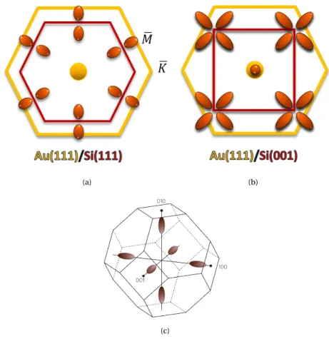
![Figure II.7: (a) Au(111)/Si(111) and (b) Au(111)/Si(001) from [51]. High elastic- elastic-current is in black and the available DOS in Si is represented by ellipses](https://thumb-eu.123doks.com/thumbv2/123doknet/14506782.720243/49.892.256.708.185.615/figure-high-elastic-elastic-current-available-represented-ellipses.webp)
![Figure V.1: Band structure of gold considering only nearest-neighbor hopping from BEEM v2.1 input files (in dashed red lines) vs second nearest-neighbor hopping from [48] (in black lines)](https://thumb-eu.123doks.com/thumbv2/123doknet/14506782.720243/99.892.243.718.197.523/figure-structure-considering-nearest-neighbor-hopping-nearest-neighbor.webp)
