Development of CMOS sensors for a future neutron eleetronie personal dosemeter

(1)

HAL Id: tel-00753855

https://tel.archives-ouvertes.fr/tel-00753855

Submitted on 19 Nov 2012

HAL is a multi-disciplinary open access

archive for the deposit and dissemination of sci-entific research documents, whether they are pub-lished or not. The documents may come from teaching and research institutions in France or abroad, or from public or private research centers.

L’archive ouverte pluridisciplinaire HAL, est destinée au dépôt et à la diffusion de documents scientifiques de niveau recherche, publiés ou non, émanant des établissements d’enseignement et de recherche français ou étrangers, des laboratoires publics ou privés.

eleetronie personal dosemeter

Ying Zhang

To cite this version:

Ying Zhang. Development of CMOS sensors for a future neutron eleetronie personal dosemeter. Other. Université de Strasbourg, 2012. English. �NNT : 2012STRAE004�. �tel-00753855�

(2)

´

Ecole Doctorale de Physique et Chimie-Physique de l’Universit´e de Strasbourg UDS

TH`

ESE

pr´esent´ee pour obtenir le grade de

Docteur de l’Universit´

e de Strasbourg

Discipline: Électronique, Électrotechnique et Automatique Spécialité : Instrumentation et Microélectronique

par

Ying ZHANG

Development of CMOS Sensors for a Future Neutron

Electronic Personal Dosemeter

soutenue publiquement le 19 septembre 2012 devant le jury: Directeurs de th`ese: M. Yann HU Pr. UDS, Strasbourg

M. Daniel HUSSON MC. UDS, Strasbourg Rapporteurs externes: M. Denis DAUVERGNE DR IPN, Lyon

M. Eric LIATARD Pr. LPSC, Grenoble

Examinateurs: M. Jean-Marc BORDY DR CEA/LNHB, Gif-sur-Yvette M. Luc HEBRARD Pr. InESS, Strasbourg

(3)

(4)

Acknowledgments

It is a pleasure to thank those who made this thesis possible. First of all, I would like to express my gratitude to my supervisors Prof. Yann Hu and Dr. Daniel Husson for giving me the opportunity to work on such exciting project and for their invaluable support, guidance and encouragement during my research. I sincerely appreciate Dr. Daniel Husson for his assistance in preparations of my manuscript by offering corrections and suggestions for improvements. I would also like to thank Dr. Christine Hu-Guo, the leader of microelectronics group, for her helpful discussions and suggestions during the prototype design.

I would like to show my gratitude to Prof. Abdel-Mjid Nourreddine, the leader of RaMsEs group for his support and for providing the proper environment for the physical experiments in this thesis.

I owe my gratitude to Anthony Bozier and Hung Pham for their fruitful discussions in the circuit design. I would like to thank Andrei Dorokhov and Min Fu for their help on device simulations. I appreciate St´ephane Higueret for his technical support during the tests and for his work in the neutron irradiation in Cadarache. I am grateful to Thˆe-Duc Le for his work in the test board design and his kind help at the beginning of the tests. I extend my gratitude to Khalil Amgarou for his valuable suggestions in the neutron measurements. Thanks also to Marie Vanstalle for her advice on experiments and data analysis.

I am grateful to all the other colleagues in PICSEL group: Marc Winter, Wojciech Dulinski, Abdelkader Himmi, Claude Colledani, Guy Doziere, Frédéric Morel, Gregory Bertolone, Isabelle Valin, Jérôm Nanni, Christian Illinger, Sylviane Molinet for their kind help, suggestions, and technical support during this thesis.

Many thanks to all the friends I met during my stay in France for the fun we shared together and for making my life here much easier.

I should not forget to thank China Scholarship Council (CSC) for their financial support. Last but not least, I would also like to thank my parents for their love, understanding, and constant support that enabled me to complete this work.

(5)

(6)

List of Figures

1.1 Energy loss for electron, muon, pion, kaon, proton, and deuteron in air as a function of their momentum [1]. . . 2 1.2 Straggling functions in silicon for 500 MeV pions, normalized to unity at the most

probable value δ/x. The width w is the full width at half maximum [2]. . . 4 1.3 Regions where the photoelectric effect, Compton effect and pair production

dom-inate as a function of the photon energy and the atomic number Z of the absorber. 7 1.4 Cross sections of the main reactions used for the detection of low-energy neutrons

[12]. . . 12 1.5 Neutron energy spectra from 25 GeV proton and electron beams on a thick copper

target. Spectra are evaluated at 90° to the beam direction behind 80 cm of concrete or 40 cm of iron. All spectra are normalized per beam particle. For readability, spectra for electron beam are multiplied by a factor of 100 [2]. . . 13 1.6 Radiation weighting factors wRfor different types of radiations from ICRP26 [19],

ICRP60 [17], ICRP103 [18]. . . 17 1.7 Electronic neutron personal dosemeters investigated in the EVIDOS survey. . . . 27 1.8 Experimental (square symbols) and simulated (lines) response functions for the

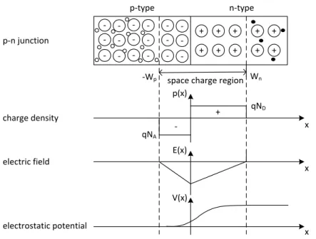
Saphydose-N (in blue) and the EPD-N2 (in red) [37]. . . 28 2.1 Approximation of an abrupt p-n junction: depletion region, space charge density,

electric field distribution, and electrostatic potential distribution. . . 36 2.2 Principle operation of a typical CMOS pixel sensor for charged particle detection.

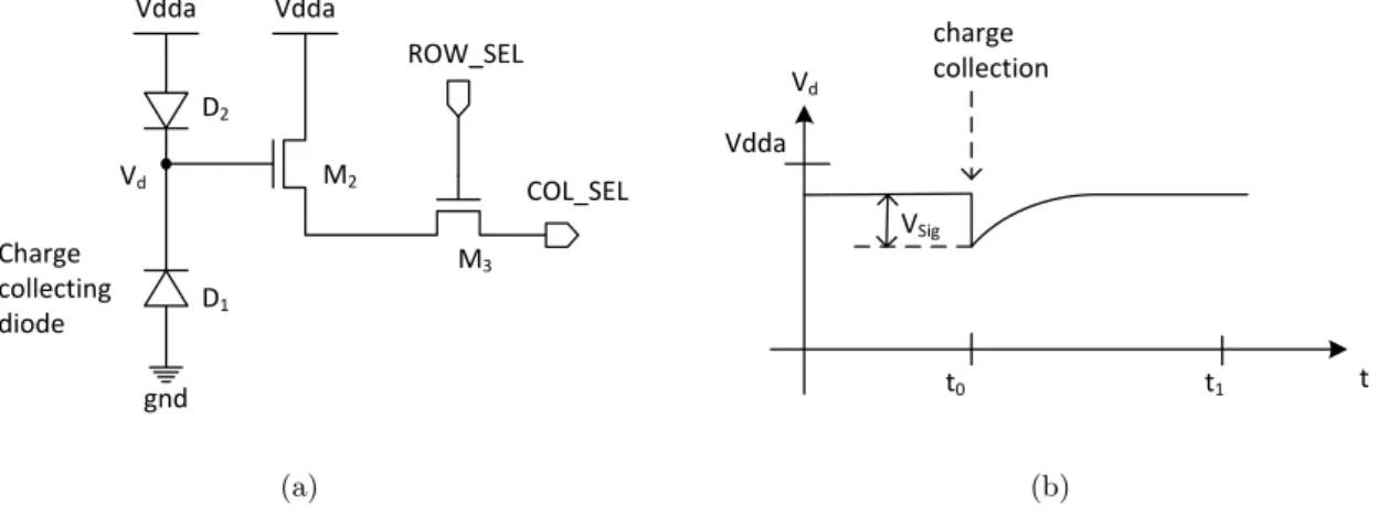
The undepleted epitaxial layer (p-epi), common in modern CMOS technologies, forms the active volume of the sensor. The charge generated in this volume by an incident charged particle diffuses thermally and is collected on an n-well/p-epi diode. Typically, the thickness of the epitaxial layer is 10-15µm [7]. . . 41 2.3 The classical single pixel cell, consisting of three transistors and the charge

col-lection diode (3T-pixel), (a) schematic, (b) timing diagram showing the operation and the signal shape. . . 42 2.4 Self-biased pixel cell (SB-pixel), (a) schematic, (b) timing diagram showing the

(11)

2.5 Block diagram of a typical CMOS pixel sensor with analog outputs. The column and row addressing shift registers sequentially select pixels for readout [2]. . . 45 2.6 Detection performances of the ULTIMATE sensor with a 20 µm thick epitaxial

layer, measured at 30 ℃ and for a power supply of 3.0 V (a) before irradiation, (b) after exposure to integrated dose of 150 kRad with 10 keV X-rays [19]. . . 47 2.7 Charge collection spectra of MIMOSA-26 sensors with (a) standard, (b) HR-15

(which has a 15 µm thick high resistivity epitaxial layer) chips. Tests with an

55_{Fe-source were performed before and after irradiation with fission neutrons [}₂₄_]. ₄₈

2.8 The substrate removal procedure includes the following steps: adding a new rein-forcing wafer, removing the original wafer body, creating deep trenches to provide contacts to the original pads, and forming a thin SiO2 entrance window [7]. . . . 49

2.9 Architecture of the MIMOSA-5 chip, (a) one chip composed of 4 pixel matri-ces of 512 × 512 pixels, (b) internal architecture of the single matrix, readout arrangement and pixel schematic diagram [28]. . . 51 2.10 Photo of the MIMOSA-5 chip . . . 52 2.11 Photo of the bonded MIMOSA-5 . . . 52 2.12 Simulated conversion efficiency as a function of the polyethylene converter

thick-ness for the AmBe and the Cf sources [32]. . . 54 2.13 Photo response of the MIMOSA-5 with and without the (CH2)n converter from

MCNPX simulations [32]. . . 55 2.14 Deposited energy distributions (normalized) simulated with MCNPX for the AmBe

mixed n/γ source (nγ/nneutrons ratio of 0.57) [36]. . . 56

2.15 Measured cluster charge distribution (in ADC) with a 90-min exposure at 15 cm from the AmBe source. The exponential and Landau-gaussian fits are respectively for the electron and the proton components [32]. . . 57 2.16 The relative efficiency and the purity of signal as functions of charge and

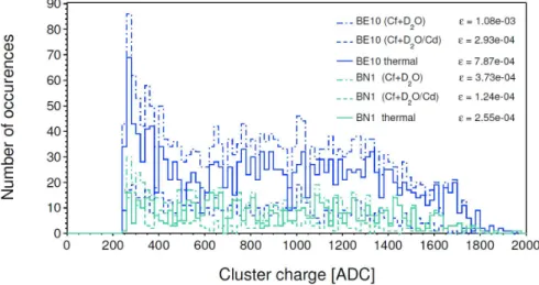
multi-plicity cuts [32]. . . 58 2.17 Simulated deposited energy for the MIMOSA-5 with BE10 and BN1 converters

exposed to the 252Cf+D2O and the (252Cf+D2O)/Cd sources. The solid lines

represent the contributions of the pure thermal neutrons [33]. . . 59 2.18 Measured deposited energy for the MIMOSA-5 with BE10 and BN1 converters

exposed to 252Cf+D2O and (252Cf+D2O)/Cd sources. The solid lines represent

the contributions of pure thermal neutrons [33]. . . 60 3.1 (a) Doping profiles used in the device simulations, as a function of wafer depth,

(b) Electron lifetime profile resulting from the doping dependence. . . 74 3.2 Transient simulation results of the two simulated structures for an given input

charge of 50 000 e-h pairs, with the inter-diode distance of (a) 80µm, (b) 100 µm. The size of the collecting diode is of 5×5 µm2 in the two cases. . . 76

(12)

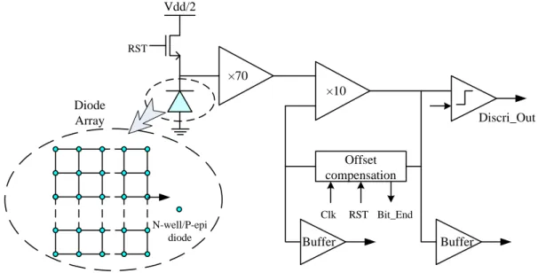
3.3 Electron concentrations for one example of the simulated structure – with a sub-strate layer of 3µm (a) at the impact time, (b) after 25 ns, (c) after 300 ns, and (d) after 1000 ns. . . 78 3.4 Substrate contribution to the total collected charge. . . 79 3.5 Architecture of the AlphaRad-1 chip, consisting of a diode array and a single

signal processing functionality accomplished by two stages of amplification, dis-crimination, and offset compensation [13]. . . 80 3.6 Simplified noise model of the analog functionality of the AlphaRad-1 chip. . . 82 3.7 Simplified noise model of the operational amplifier used in the AlphaRad-1 chip. 83 3.8 Simplified noise model of the DAC in the offset-compensation system. . . 84 3.9 Schematic diagram of the current mode signal processing architecture. . . 86 3.10 DC-voltage distributions of the nodes (a) I out and (b) Out shown in Fig. 3.9. . 87 3.11 DC-voltage compensation system for the node I out. . . 88 3.12 DC-voltage compensation system for the node Out. . . 88 3.13 Transient response of the compensation systems for the node I out (upper) and

Out (lower) with a clock of 500 kHz. . . 89 3.14 DC-voltage distributions of the node I out, (a) without compensation, (b) with

compensation. . . 89 3.15 DC-voltage distributions of the node Out, (a) without compensation, (b) with

compensation. . . 90 3.16 Noise model of the current readout stage for each row. . . 90 3.17 Noise model of the current-to-voltage stage and the voltage amplifier for the full

matrix. . . 91 3.18 SNR dependence on the diode matrix size for the voltage mode (solid line) and

current mode (dashed line) signal processing architectures. . . 93

4.1 Architecture of the proposed compact device based on CMOS sensors for opera-tional neutron dosimetry. . . 98 4.2 Total output current of a 4 × 4 diode cluster, with the diode size of 5×5µm2 and

an inter-diode distance of 80 µm. . . 99 4.3 Total output current of a 4 × 4 diode cluster, with simulated points, and our

exponential model. The corresponding collected charge is about 5.83 fC. . . 100 4.4 Principle schematic of the charge sensitive amplifiers with (a) an infinite, and (b)

a finite integration time. . . 101 4.5 Normalized CSA output pulses for an unit input charge with different integration

time. The later choice (12µs) is depicted by a solid line. . . 103 4.6 The commonly used single-ended amplifier configurations: (a) the “direct” cascode,

(b) the “folded” cascode. . . 104 4.7 Schematic of the single-ended input split-leg cascode amplifier, where the voltage

(13)

4.8 Small-signal model of Fig. 4.7 for (a) gain analysis, and for (b) noise analysis, where the source follower and the bulk effect on M1 and M2 are neglected . . . . 106

4.9 Schematic of the shaper with the active feedback. . . 109 4.10 Noise equivalent model for the CSA and the shaper with the detector capacitance

input load. . . 110 4.11 Schematic of the hysteresis comparator using the internal positive feedback. . . . 112 4.12 Simulated transfer curve of the hysteresis comparator with a 10 pF load. . . 114 4.13 Layout of the readout circuit, containing CSA, shaper, discriminator and analog

buffers. . . 114 4.14 Layout of the AlphaRad-2 chip. . . 115 4.15 Transient response of the chip to the input signal (charge of 5.83 fC) in Fig. 4.3

from the post-simulation. . . 116 4.16 Photo of the wire bonded AlphaRad-2 chip . . . 116 4.17 Photo of the test board . . . 116 4.18 Measured waveform of the chip’s response to an injected charge of 5.83 fC: at the

output of CSA (upper curve), shaper (middle curve), and discriminator (lowest curve). . . 117 4.19 Measured versus simulated signal amplitudes at the output of shaper with

dif-ferent input charges. (The vertical uncertainties for the measurement are in the level of some millivolts so that they are invisible due to the scale). . . 118

5.1 Diagram of the acquisition system for the analog signal analysis. . . 122 5.2 Signal distribution at the output of the shaper from the acquisition in the dark.

The mean value represents the baseline, and the RMS is the total electronic noise. 122 5.3 Ranges of the 5.5 MeV α-particles traveling in the CMOS sensor simulated by

SRIM for four sensor-source distances. . . 124 5.4 Photos of the experimental setup: (a) overall view of the setup, showing the barrel

containing the source and the sensor, mother-board, power supply and controlled computer; (b) inside of the barrel, showing the base plate holding the source and the AlphaRad-2 test board. . . 125 5.5 Distributions of the detected charge obtained for an exposure of 2 minutes with

the241Am source at the four working distances. . . 125 5.6 Counting rate of the 241Am α-measurements versus geometric calculation as a

function of the source-sensor distances [2]. . . 126 5.7 Measured charge distributions with and without the aluminium shield for a 50

min-utes exposure at 1 cm from the 137Cs source. . . 127 5.8 Spectra of the neutron sources at the IRSN. . . 128 5.9 Photo of the Van Gogh irradiator [4]. . . 129 5.10 Distributions of the detected charge for a 310-min exposure at 20 cm from the

(14)

5.11 Measured charge distribution for a 140-min exposure at 20 cm from the241AmBe

source. . . 131

5.12 Distributions of the detected charge for a 310-min exposure at 20 cm from the 241_{AmBe source with two converters: a graphite foil (C) and a polyethylene (PE)} converter. . . 131

5.13 Distributions of the detected charge for a 310-min exposure at 20 cm from the 241_{AmBe source. The two fitting functions are presented: the Landau-gaussian} (in blue) for proton distribution and the exponential (in orange) for electron distribution. . . 133

5.14 The relative efficiency and the purity of signal as a function of charge cut (only statistical uncertainty is included in the error bars). . . 133

5.15 Normalized charge distributions measured at the distance of 20 cm and 75 cm from the AmBe source on the Van Gogh irradiator. . . 135

5.16 Dose response function of AlphaRad-2 measured with the AmBe source at the IRSN (10 Ci activity). . . 136

5.17 Schematics of the241AmBe source at IPHC, showing (a) geometry, (b) dimensions of the source (the values are given in mm) [3]. . . 137

5.18 Photo of the experimental setup for the measurements with the AmBe source at IPHC. . . 137

5.19 Measured charge distributions for different polyethylene converter thicknesses dur-ing the 21 hours exposure at 8.2 cm from the AmBe source at IPHC. . . 138

5.20 Dependance of the detection efficiency to the polyethylene converter thickness measured at 8.2 cm from the IPHC AmBe source. . . 139

5.21 Measured charge distributions (normalized by their respective exposure time) for different distances from the AmBe source at IPHC. . . 139

5.22 Distance dependance of the intrinsic detection efficiency measured with the AmBe source at IPHC. . . 140

A.1 First page of the schematic of the AlphaRad-2 test board. . . 148

A.2 Second page of the schematic of the AlphaRad-2 test board. . . 149

A.3 Third page of the schematic of the AlphaRad-2 test board. . . 150

A.4 Forth page of the schematic of the AlphaRad-2 test board. . . 151

(15)

(16)

List of Tables

1.1 Classification of neutrons based on their energies. . . 9

1.2 Radiation weighting factors wR from ICRP103 [18]. . . 18

1.3 Tissue weighting factors wT from ICRP103 [18]. . . 19

1.4 Operational quantities for different radiation protection tasks. . . 21

1.5 Characteristics of the electronic neutron personal dosemeters tested in the EVI-DOS survey. . . 27

2.1 Measured and simulated γ-response for the MIMOSA-5 to 60Co source (the re-sponse Rγ is defined as the ration of γdetected on γincident, while Edep represents the deposited energy). Uncertainties are statistical [32]. . . 55

2.2 Measured and simulated detection efficiencies with the MIMOSA-5 to252Cf+D2O and (252Cf+D2O)/Cd sources using two types of converters [32]. . . 59

3.1 Charge collection properties in the given simulated volume (320×320×14 µm3) with different geometric parameters [12]. The collection time is defined as the time after which 90% of the total charges is collected. . . 77

4.1 The performance comparison of the two AlphaRad chips. . . 118

5.1 Elemental analysis results of the graphite and polyethylene converters. . . 130 5.2 Fitting parameters for the charge distribution with the AmBe source (Fig. 5.13). 132 5.3 The relative efficiencies and signal purities for different applied ADC charge cuts. 133

(17)

(18)

R´

esum´

e en Fran¸

cais

Les radiations ionisantes sont bien connues pour causer des dommages aux cellules vivantes et aux dispositifs électroniques à base de silicium. Au total, ce sont 63000 travailleurs en Europe qui sont exposés à ces rayonnements, dans les installations nucléaires ainsi que, de plus en plus, en milieu médical. La mesure quantitative des doses absorbées est réalisée par différents types de dosimètres, selon le type de radiation (X, β, γ, n). Les neutrons présentent les plus grandes difficultés de mesure au niveau des doses, car, électriquement neutres, ils ne sont pas directement détectables, mais seulement au travers des particules secondaires qu’ils créent par réactions nucléaires ou simple diffusion. De plus, on les trouve sur une gamme d’énergie extrêmement ´

etendue, qui va du meV au GeV, avec des effets biologiques tr`es fortement d´ependants de leur ´

energie. Il est donc essentiel pour un dosimètre de distinguer les neutrons de basse énergie des neutrons rapides (>100 keV). En dernier lieu, les neutrons apparaissent toujours en champs mixtes n-γ, la tâche d’un bon dosimètre est alors d’opérer une claire distinction entre les deux. A l’heure actuelle, seuls les dosimètres passifs, qui intègrent la dose, sont considérés comme fiables pour la mesure de neutron, les dosimètres opérationnels ne donnant pas de résultats satisfaisants, alors qu’une telle mesure est obligatoire pour tous les travailleurs du nucléaire depuis 1995 (circulaire IEC1323).

Au sein de l’IPHC (Institut Pluridisciplinaire Hubert Curien) le groupe RaMsEs a donc pro-posé une solution en propre, basée sur la technologie des capteurs CMOS (« Complementary Metal Oxyde ») pour lesquels le laboratoire possède une expertise de niveau mondial. Une dé-cennie de développements, motivée par la physique des particules (projet ILC) a fait émerger d’autres applications possibles. En particulier, ces capteurs présentent des caractéristiques in-téressantes pour la détection efficace des neutrons : faible consommation électrique, bas coût, portabilité, volume limité (d’où une sensibilité aux photons presque nulle) ainsi qu’une pos-sibilité d’intégration complète de l’électronique de traitement. Une étude préliminaire a déjà ´

eté conduite au RaMsEs, avec un vrai capteur à pixels, le MIMOSA-V (« Minimum Ionising particle MOS sensor ») développé pour la trajectographie des particules de haute énergie. Il a ´

eté démontré qu’une coupure adéquate rendait bien le capteur transparent aux γ, sans perte de signal. L’efficacité de détection aux neutrons rapides, de l’ordre de 10−3, est celle attendue par simulation, et quasiment identique à l’efficacité aux neutrons lents (convertisseur au bore), résultats qui laissent présager une réponse constante sur toute la gamme des énergies. Malgré

(19)

ces résultats prometteurs pour la dosimétrie neutron, le MIMOSA-V ne saurait être la solution pour un dosimètre, à cause de l’encombrement actuel du système complet (qui doit devenir un vrai système intégré) et au vu de l’énorme flux de données généré sur une courte période par un quart de million de pixels.

Cette thèse présente donc le développement d’un système miniaturisé pour la dosimétrie neutron sur la base des acquis en capteurs à pixels. Un circuit dédié, AlphaRad-2, a été con¸cu et implémenté en technologie AMS 0.35 (Austria MicroSystems), circuit CMOS à très faible consommation et alimenté en 2.5 V.

La th`ese est organis´ee selon le plan suivant:

Chapitre 1 : présentation de la physique de l’interaction rayonnement-matière, et problèmes généraux de détection. Nous discutons aussi les interactions photons ainsi que des particules secondaires. Dans une seconde partie, nous présentons les grandeurs associées à la mesure des doses définies par l’ICRP (International Commission on Radiological Protection), ainsi que les méthodes spécifiques de détection des neutrons.

Chapitre 2 : les principes de base de détection de particules ionisantes dans un détecteur silicium sont passés en revue. Après un résumé de la décennie de développement des capteurs pixels (CPS) pour la physique des particules (détecteurs de vertex), on exposera les résultats du MIMOSA-5 aux neutrons, ainsi que les faiblesses du système.

Chapitre 3 : l’idée originale d’une architecture en « mono-pixel » est explicitée dans un premier temps. Une étude complète de simulation avec la suite Sentaurus-TCAD a été conduite pour comprendre le processus de collection de charge (efficacité et temps caractéristique). Nous détaillons ces résultats, essentiels pour fixer les paramètres du capteur (taille de la micro-diode ´

elémentaire, espacement). S’en suit l’analyse des différents étages de traitement électronique, incluant une discussion des architectures « tension » ou « courant ».

Chapitre 4 : un circuit dédié, AlphaRad-2, pour un futur dosimètre électronique personnel de neutrons est proposé. Ce chapitre se penche sur l’étude théorique complète de l’électronique de lecture, présentée avec les résultats de tests électroniques.

Chapitre 5 : ce chapitre est consacré à des tests de notre prototype sous différents types de rayonnement, avec en première partie la réponse à une source alpha pour l’étalonnage du taux de comptage. Nous présentons également une mesure de la sensibilité aux électrons, aux neutrons rapides ainsi que la procédure pour distinguer photons et neutrons. En tout dernier lieu, nous abordons l’influence de l’épaisseur de convertisseur polyéthylène et la réponse du capteur en fonction de la distance.

Pour finir, le dernier chapitre présente les conclusions générales de ce développement, avant d’introduire une perspective de grand intérêt : en 2012, nous avons transposé l’architecture de l’AlphaRad-2 dans un « process » de fabrication nouveau (XO035 de X-FAB), qui doit permettre de décliner la plage à neutrons lents de manière telle à éviter, dans le futur, de devoir amincir le capteur.

(20)

Introduction

It is universally acknowledged that radiation causes damage, which can range from a subtle cell mutation in a living organism to the bulk damage in a silicon detector. About 63000 workers in Europe are exposed to the risk posed by these harmful radiation, mainly in nuclear power plans and in medical therapy facilities. Quantitative measurement of the dose absorbed by an organism is provided by dosemeters. There are different types of dosemeters according to the detected radiation (γ, β, X, n,. . .). Neutrons, are well-known to be an even more troublesome particle species with respect to dosimetry. Firstly, they are electrically neutral, so that they are not affected by electromagnetic forces and unable to directly ionize matter. In fact, detection of neutrons is only possible through the secondary charged particles released from their nuclear interactions in a given material. Moreover, neutrons exist over a wide energy range from meV to GeV, and their biological effects on life beings are different according to their energies. It is therefore essential for a dosemeter to be able to differentiate low energy neutrons from fast neutrons (En >100 keV). Finally, neutrons are always accompanied by γ radiation, leading to

n-γ mixed fields. A neutron dosemeter has to recognize neutrons in the presence of photon and electron radiations. Currently, only the passive dosemeters, providing an integral on the dose to an individual over the wearing period, are considered reliable in neutron dosimetry. Active dosemeters (giving the dose information “online”) exist, but do not yet give results as satisfactory as passive devices. Their use, however, became mandatory for workers in addition to the passive dosimetry since 1995 (IEC 1323).

Therefore, the RaMsEs group in the laboratory IPHC (Institut Pluridisciplinaire Hubert Curien, UMR 7178) proposed its own solution to active neutron dosemeters, based on a new technology in the field of dosimetry: CMOS (Complementary Metal Oxide Semiconductor) tech-nology, in which IPHC has a world-class expertise. More than a decade has passed since the first CMOS sensor was developed for charged particle tracking, motivated by the linear collider project. Numerous other applications have emerged since then. These sensors present attrac-tive characteristics for neutron dosimetry: low power consumption, low cost, portability, a thin sensitive volume which implies a low sensitivity to photons and the full integration of the read-out electronics on the same substrate as the sensing elements. To investigate the feasibility of CMOS technology for the application in neutron dosimetry, a previous study had been done by the RaMsEs group. Extensive experiments had been performed with a true pixelated CMOS

(21)

sensor, MIMOSA-5, (Minimum Ionizing particle MOS Active pixel sensor), originally designed for particle tracking. It has been demonstrated that by applying an appropriate threshold the sensor can be considered as γ-transparent. The measured efficiency to fast neutrons is of the same order of magnitude (10−3) as that to thermal neutrons obtained using a natural boron converter. These results are encouraging to obtain a constant response of the detector with the energy of the incident neutrons. The study with the MIMOSA-5 sensor provided experimen-tal evidence that CMOS sensors offer promising characteristics in the application to neutron dosimetry. However, the MIMOSA-5 sensor can not be used directly for a personal dosemeter due to a major drawback: its pixelation makes the data stream too large to develop a portable integrated system (system-on-chip) where data is directly processed.

The work presented in this thesis addresses the development and characterization of an efficient and miniaturized system based on a dedicated CMOS sensor for a future neutron per-sonal dosemeter. Based on the results obtained with the MIMOSA-5, a new dedicated sensor AlphaRad-2, with very low power consumption, has been implemented in the AMS (Austriami-crosystems AG) 0.35 µm CMOS technology with a 2.5 V power supply.

This thesis is organized as follows:

• In chapter 1, the physics of the interactions of radiation with matter, which the detection of particles is based on, will be presented. We make an overview of interactions of photons and the secondary charged particles that were encountered during this work. The second part of the chapter focuses on the radiation dosimetry in general by introducing a series of dosimetric quantities defined by the International Commission on Radiological Protection (ICRP). Finally, the methods currently used in neutron dosimetry will be described. • In chapter 2, basic physics principles governing charge generation and collection in silicon

detectors after a passage of an ionizing particle will be presented. Development of CMOS Pixel Sensor (CPS) for vertex detectors at IPHC in the past more than ten years will be the second part of this chapter. The third part presents the experimental measurements of the MIMOSA-5 sensor with fast and thermal neutrons. The possibilities and the weak points of the sensor are identified.

• In chapter 3, the idea of using an equivalent “mono-pixel” architecture as the sensing part for dosimetric applications is described in the beginning. Device physics simulations by means of the Sentaurus-TCAD (Technology Computer-Aided Design) tool targeting on the study of charge collection in micro-diodes will be given. We detail the simulation results in order to set the sensor parameters (size of the micro-diode, inter-diode distance). The charge collection simulation is followed by the analysis and design of the two different signal processing architectures, including the voltage mode and the current mode.

• In chapter 4, a dedicated CMOS sensor, AlphaRad-2, for a future neutron personal doseme-ter is proposed. The design of a low-noise, low-power consumption readout circuit is pre-sented for both its theoretical analysis and electrical test results.

(22)

are presented. The first part shows the results of measurements made to test the sensor in detection efficiency by the exposure to α particles. It also summarizes the results of experiments performed to determine the sensor sensitivity to photons and fast neutrons as well as a n/γ discrimination threshold. The last part of this chapter covers the study on the influence of the thickness of polyethylene converters and the sensor response as a function of distance.

• In the conclusion, the results obtained in this thesis will be summarized and the main con-clusions will be presented. At the end, the perspectives for using CMOS sensors in neutron dosimetry are addressed. To improve the detection performance and exploit the possibility of detecting thermal neutrons without thinning down the standard sensor, we present a reproduction of the AlphaRad-2 in a specialized process for optoelectronic applications (XO035 technology, X-FAB).

(23)

(24)

Chapter 1

Neutron interactions and dosimetry

The detection of neutrons requires not only to know the interaction probability with matter but also the knowledge of the interactions of the related particles with matter, i.e. the secondary charged particles (α, protons) generated by neutrons along their paths. In addition, we need a good knowledge of the particles that make up the physical background of the signal (i.e. photons, in our case). We start this chapter with the review of the interaction mechanisms of the related particles.

1.1 Interactions of particles with matter

Particles and radiation can be detected only through their interactions with matter. The way particles interact with matter depends not only on the types of incident and target particles but also on their properties, such as energy and momentum. There are two main kinds of processes by which a particle going through matter can lose energy. In the first kind the energy loss is gradual, which is the case for charged particles. In the second kind the energy loss happens as single event; for instance, a photon moves without any interaction at all through the material until, most of the time in a single collision, it loses all its energy. The neutron itself is an intermediate case, able to lose energy in several collisions before undergoing a single inelastic event. In this section, we will start by considering the interaction of heavy charged particles with matter, and then proceed to look at the interaction of electrons and photons.

1.1.1 Interaction of heavy charged particles

The moving charged particles exert electromagnetic forces on atomic electrons and impart energy to them. A heavy charged particle travels with an almost straight path through matter, losing its energy gradually.

(25)

1.1.1.1 Energy loss

The main interactions of heavy charged particles with matter are ionization and excitation. The mean rate of energy loss (or stopping power) by moderately relativistic charged heavy particles is well-described by the Bethe-Bloch equation

−dE dx = Kz 2Z A 1 β2[ 1 2ln 2mec2β2γ2Tmax I2 − β 2₋δ(βγ) 2 ] (1.1) where

z – charge of the incident particle in units of the elementary charge; Z, A – atomic number and mass of the absorber;

me – electron mass, mec2= 0.510 MeV;

re – classical electron radius, re = 2.817 × 10−15 m;

NA – Avogadro’s number, NA = 6.022 × 1023 mol−1;

I – mean excitation energy in units of eV;

β – velocity of the particle in units of speed of light, β = ν/c; γ – the Lorentz factor, γ = √1

1−β2;

δ(βγ) – density effect correction to ionization energy loss; K/A = 4πNAr2emec2/A = 0.307 MeV g−1cm2 for A = 1 g mol−1.

Tmax is the maximum kinetic energy which can be imparted to a free electron in a single

collision and given by

Tmax=

2mec2β2γ2

1 + 2γme/M + (me/M )2

(1.2)

where M is the mass of the incident particle.

Figure 1.1: Energy loss for electron, muon, pion, kaon, proton, and deuteron in air as a function of their momentum [1].

(26)

Equation (1.1) describes the mean rate of energy loss in the region 0.1 . βγ . 1000 for intermediate-Z materials with an accuracy of a few percent. At the upper limit, radiation losses begin to be important, at at lower energies, the projectile velocity becomes comparable to atomic electron “velocities” [2]. Both limits are Z dependent. In the region of Bethe-Bloch, the energy loss is decreasing as 1/β2 until it reaches the minimum at βγ ≈ 3. Particles with this minimum amount of energy loss are referred to as Minimum Ionizing Particles (MIPs). Figure 1.1 shows the ionization energy loss for electrons, muons, pions, kaons, protons and deuterons in air. As their energy loss curves are well separated, these particles can be discriminated according to their deposited energy. However, this discrimination is no longer achievable for βγ values above 3.

As the particle energy increased, its electric field flattens and extends, so that the distant-collision contribution to Bethe-Bloch equation increased as ln βγ. Another effect responsible for the relativistic rise originates from the β2γ2 growth of Tmax, which is due to (rare) large energy

transfers to a few electrons. When these events are excluded, the energy deposit in an absorbing layer approaches a constant value [3].

For energy loss at low energies shell corrections must be included in the square bracket of Eq. (1.1) to correct for atomic binding. A detailed discussion of low-energy corrections to the Bethe formula can be found in [4]. When the correction are properly included, the Bethe treatment is accurate to about 1% down to β ≈ 0.05, or about 1 MeV for protons.

For 0.01< β < 0.05, there is no satisfactory theory. For protons, one usually relies on the phenomenological fitting formulae developed by Andersen and Ziegler [4,5].

The energy loss is a stochastic process because of two sources of variations: the transferred energy in a single collision and the actual number of collisions. The fluctuation of the num-ber of collisions can be described by the Poisson law. The quantity (dE/dx)δx represents the mean energy loss via interactions with electrons in a layer of thickness δx. For finite thickness, strong fluctuations around the average energy loss exist. The energy-loss distribution is strongly asymmetric, skewed towards high values. For detectors of moderate thickness x, the energy loss probability distribution is firstly described by the Landau distribution [6]. The Landau distribu-tion is not an accurate descripdistribu-tion of the energy loss in thin absorbers, such as silicon detectors (i.e. CMOS sensors). While the most probable energy loss can be calculated adequately, its distri-bution becomes significantly wider than the Landau width [2]. Thinner absorbing layers exhibit a larger deviation from the Landau distribution, and the most general model to be applied is the Vavilov theory. Figure 1.2 presents the energy loss distributions for 500 MeV pions incident on thin silicon detectors. The position of the peak in the distribution defines the most probable energy loss. The mean energy loss is shifted to a higher energy.

In reality, detectors only measure the energy which is actually deposited in their sensitive volume rather than the total energy loss by the impinging particle. Some of the energy lost by an impinging particle is carried away by knock-on electrons (δ-rays) or by fluorescence photons or in a much less extent by Cherenkov radiation and Bremsstrahlung.

(27)

100 200 300 400 500 600 0.0 0.2 0.4 0.6 0.8 1.0 0.50 1.00 1.50 2.00 2.50 640 μm (149 mg/cm2) 320 μm (74.7 mg/cm2) 160 μm (37.4 mg/cm2) 80 μm (18.7 mg/cm2)

500 MeV pion in silicon

Mean energy loss rate w f (Δ /x ) Δ/x (eV/μm) Δp/x Δ/x (MeV g−1 cm2)

Figure 1.2: Straggling functions in silicon for 500 MeV pions, normalized to unity at the most probable value δ/x. The width w is the full width at half maximum [2].

1.1.1.2 Energy-range relation

The range R(E) of a charged particle of kinetic energy E0 is the integral of the stopping

power over the full energy spectrum of the incident particle

R(E) = Z E0

0

dE

−dE/dx (1.3)

Because of the fluctuations of the energy loss and the multiple Coulomb scattering in the material, the range of charged particles in matter shows statistical fluctuations around a mean value, termed as range straggling. Equation (1.1) may be integrated to find the total (or partial) CSDA (Continuous Slowing Down Approximation) range R for a particle which loses energy only through ionization and atomic excitation. However, since the energy loss is a complicated function of the energy, in most cases approximations of this integral are used. Experimentally, some empirical and semi-empirical formulae have been proposed for certain particle species in the given energy ranges.

Range of α-particles Several empirical and semi-empirical formulae have been given to cal-culate the range of α-particles in air. For example [7]

R_αair=   

0.56Eα for Eα< 4 MeV

1.24Eα− 2.62 for 4 MeV ≤ Eα≤ 8 MeV

(28)

where the kinetic energy Eα is in MeV, and the Rairα is in cm.

The range of α-particles in other materials obeying scale law can be roughly estimated by

Rα= 3.37 × 10−4Rαair

√ A

ρ (1.5)

where A (g/mol) is the atomic weight, and ρ (g/cm3) is the density of the material, respectively.

Range of protons In air the range (in cm) of protons having energy Ep can be described by

Eq. (1.6) [8]

Rair_p = 100 · (Ep 9.3)

1.8 _{0.6 MeV ≤ E}

p ≤ 20 MeV, (1.6)

while for aluminum, one can use Eq. (1.7) [9] RAl_p =

  

3.837E_p1.5874 for 1.13 MeV < Ep ≤ 2.677 MeV 2.837E2

p

0.68+log Ep for 2.677 MeV ≤ Ep ≤ 18 MeV,

(1.7)

where the RAl_p is given in mg/cm2.

1.1.2 Interaction of electrons

There is a significant difference between electron and heavy charged particle behaviors when passing through matter. The way an electron interacts with matter depends, to a large extent, on its energy. At low to moderate energies, the primary types of interaction are: ionization, Moeller scattering, and Bhabha scattering. At higher energies the Bremsstrahlung process dominates the energy loss.

1.1.2.1 Energy loss

Ionization energy loss by electrons differs from loss by heavy particles because in the case of electrons the mass of the incident particle and the target electron are the same. Apart from this interaction process, the incident electron interacts with the nucleus of the absorber atom via Bremsstrahlung resulting in abrupt changes in the electron direction. Hence the stopping power for electrons consists of two components, collisional and radiative

(dE dx)tot = ( dE dx)coll+ ( dE dx)rad (1.8)

where coll denotes the collisional term due to ionization and excitation, and rad denotes the radiative term due to electromagnetic radiation. The collisional energy loss rate rises logarith-mically with energy, while bremsstrahlung losses rise nearly linearly, and dominate above a few tens of MeV in most materials.

(29)

1.1.2.2 Passage of electrons

The trajectory of an electron is often erratic and winding, due to the fact that it will experi-ence multiple scattering and will suffer Bremsstrahlung in the absorber. The mean free path is then defined as the thickness of a material which reduces the intensity of a monoenergetic beam of electrons to half. To estimate the value of this path, there is no analytical formula but only empirical formulas. For example, the expression is given by Katz and Penfold [10]

Rmax =

  

0.412E1.265−0.0954 ln(Ee)

e for 10 keV ≤ Ee≤ 2.5 MeV

0.530Ee− 0.106 for 2.5 MeV ≤ Ee≤ 20 MeV

(1.9)

where the maximum range Rmax is in g/cm2, and the energy Ee is in MeV.

1.1.2.3 Radiation length

High energy electrons predominantly lose energy by Bremsstrahlung. The energy loss by Bremsstrahlung can be described by

E = E0e−x/X0 (1.10)

where E0 is the energy of the incident electron, and x/X0 is the thickness of the scattering

medium, measured in units of radiation length X0. The radiation length X0 is defined as the

mean distance over which a high-energy electron loses 1 − 1_e of its energy by Bremsstrahlung. The radiation length X0, usually measured in g/cm2, is a property of the material. A good

approximation is given by Dahl [11] X0 =

716.4 · A

Z(Z + 1) ln(287/√Z) (1.11)

where A, Z are the atomic weight and atomic number of the medium, respectively.

1.1.3 Interaction of photons

Photons are detected indirectly via interactions with the medium of the detector. In our energy range of interest, photons interact with matter by mainly three processes: photoelectric effect, Compton effect and pair production. These interaction processes have different energy thresholds and high cross-sections regions for different materials. The relative importance of these three interactions is a function of the energy of incident photon and of the atomic number of the detector material, as shown in Fig. 1.3. In every photon interaction, the photon is either completely absorbed or scattered. In the following, we describe with more details these different processes.

(30)

Figure 1.3: Regions where the photoelectric effect, Compton effect and pair production dominate as a function of the photon energy and the atomic number Z of the absorber.

1.1.3.1 Photoelectric effect

This effect predominates for photons of energy below 100 keV (or 300 keV for heavy material). In the photoelectric interaction, the photon is absorbed by the atom, generating photoelectron. Since an atom is much more massive than an electron, the ejected electron takes practically all the energy and momentum of the photon. The kinetic energy of the ejected electron (Epe) is

determined by the electron binding energy (EB), as described by Eq. (1.12).

Epe = hν − EB (1.12)

where hν is the kinetic energy of the incident photon. If the resulting photoelectron has sufficient kinetic energy, following secondary ionization may occur along its trajectory. The vacancy created by the emission of the photoelectron is immediately filled by another atomic electron, emitting then either a characteristic X-ray or an Auger electron. If these radiations are stopped within the detector material, then the deposited energy corresponds to the full energy of the incident photon. This feature of the photoelectric effect allows to calibrate the gain of the detector with its readout system if the required energy for creating a single electron-hole pair is known. The mass attenuation coefficient for photoelectric absorbtion decreases with the increase of the photon energy. For a given value of energy, the attenuation coefficient increases with the atomic number Z of the material. The relevant cross section σpe can be approximated by

σpe∝

Z4.35

(hν)n (1.13)

(31)

1.1.3.2 Compton effect

Compton effect becomes significant for photons of energy between 100 keV and 5 MeV(or 10 MeV for light materials). The Compton effect is the scattering of photons off quasi-free atomic electrons. Part of the energy of the photon (hν) is transferred to the emitted electron, and its direction is changed. The energy of the scattered photon E_γ0 = hν0 is given by

E_γ0 = hν

1 + η(1 − cos θ) (1.14)

where η = hν/mec2 with mec2 = 511 keV, and θ is the scattering angle of the photon. The

secondary electron is ejected with an angle ϕ with respect to the direction of the incident photon, and its kinetic energy Ee given by Eq. (1.15).

Ee=

η(1 − cos θ)

1 + η(1 − cos θ)hν (1.15)

with a simple relationship between the angles θ and ϕ: cos ϕ = (1 + θ) tan (θ/2).

1.1.3.3 Pair production

If the photon energy reaches more than 1.022 MeV, the production of electron-positron pairs in the Coulomb field of a nucleus or an electron is possible. The threshold energy is given by the rest masses of two electrons plus the energy transferred to the nucleus or electron. Consequently, the effective threshold is about 2mec2 (1.022 MeV) or 4mec2 (2.044 MeV) for the interaction

with a nucleus or an electron, respectively.

1.1.3.4 Attenuation of photons

When a monoenergetic beam of photons with intensity I0 strikes the detector material of

thickness x, the intensity of photons, I(x), penetrating without any interaction is given by

I(x) = I0e−µlx (1.16)

where µl (in m−1 or cm−1) is the linear attenuation coefficient, describing the probability of

interaction per unit distance. A more useful quantity, the mass attenuation coefficient µm is

defined as µl/ρ (with ρ is the density of the material). µm is related to the cross section for the

various interaction processes of photons according to

µm= NA A X i σi. (1.17)

where σi is the atomic cross section for the process i, A is the atomic weight and NA is the

(32)

fact like the various cross sections.

1.1.4 Interaction of neutrons

Neutrons, being uncharged, undergo extremely weak electromagnetic interactions, therefore pass through matter largely unimpeded, only interacting with atomic nuclei. As they are highly penetrating and can induce secondary deep body ionizing radiation doses, the health risk asso-ciated with neutrons is significant.

1.1.4.1 Classification of neutrons

Neutron reactions can take place at any energy, and the interaction type strongly depends on neutron energy. Neutrons are usually classified on the basis of their kinetic energies but without clear established limits. Table 1.1 summarizes the main categories that are commonly used in neutron dosimetry:

Type of neutrons Energy Ultra-cold < 100 neV

Cold < 25 meV

Thermal 25 meV – 1 eV

Intermediate 1 eV – 100 keV

Fast 100 keV – 20 MeV

Relativistic 20 MeV – 1 GeV Ultra-relativistic 1 GeV – 10 TeV

Table 1.1: Classification of neutrons based on their energies.

1.1.4.2 Cross sections of neutrons

The probability of a particular reaction occurring between a neutron and an individual particle or nucleus is defined through its microscopic cross section (σ). It is dependent not only on the kind of nucleus involved, but also on the energy of the neutron. Another cross section, known as the macroscopic cross section (Σ), is defined to describe the probability per unit path length that a particular type of interaction will occur. The macroscopic cross section (Σ) is related to the microscopic cross section (σ) by

Σ = N σ (1.18)

where N is the atom density of the material (atoms/cm3). All process can be combined to calculate the total probability per unit path length that any type of interaction will occur by

(33)

the Eq. (1.19).

Σtot = Σsca+ Σabs (1.19)

where Σsca, Σabs represent the macroscopic cross section for scattering and absorption,

respec-tively.

1.1.4.3 Different types of interactions

This section introduces five reactions that can occur when a neutron interacts with a nucleus. In the first two, known as scattering reactions, a neutron emerges from the reaction. In the remaining reactions, known as absorption reactions, the incoming neutron is absorbed by the nucleus with the emission of secondary particles. For fast and thermal neutrons, scattering and absorption reactions are prominent, respectively.

Elastic scattering (n,n) Elastic scattering, being the principle mode of interaction of neu-trons with atomic nuclei, occurs at all neutron energies. A neutron collides with a nucleus, transfers some energy to it, and bounces off in a different direction. The amount of kinetic en-ergy transferred to the target strongly depends on the nucleus mass and the angle of impact. Elastic scattering is the most likely interaction between fast neutrons and low mass absorbers. For an elastic collision by conservation of the momentum and the kinetic energy, the kinetic energy of the recoil nucleus Er is given by

Er = En·

4A (1 + A)2(cos

2_θ) _(1.20)

where En is the energy of the incident neutron, θ is the angle between the recoil and the target

nucleus in the laboratory system, and A is the ratio of the mass of the target nucleus to the neutron mass. Fast neutron detectors take advantage of the fact that a fraction of the neutron’s kinetic energy can be transferred to the target nucleus producing an energetic recoil nucleus. When a hydrogen absorber (A = 1) is used, the transferred energy to the recoil proton increases to Ep = Encos2θ. This indicates that the fast neutrons could transfer all their energy in a single

interaction with the hydrogen nucleus (proton). This reaction is the main process used for the fast neutron detection in Chapter 5 of this work.

Inelastic scattering (n,n’) Inelastic scattering is similar to elastic scattering except that the nucleus undergoes an internal rearrangement into an excited state from which it subsequently emits γ-rays. The total kinetic energy of the outgoing neutron and nucleus is much less than the kinetic energy of the incoming neutron, because part of the original kinetic energy is used to excite the compound nucleus. The emitted neutron may or may not be the incoming one. The average energy loss depends on the energy levels of the target nucleus. The inelastic scattering can occur only if the energy of the incoming neutron reaches the required energy for exciting the

(34)

target nucleus. This threshold energy depends on the type of nucleus. In particular, the inelastic scattering with hydrogen is impossible since the hydrogen nucleus does not have excited states.

Radiative capture (n,γ) In this process, the nucleus is excited but the level of excitation is insufficient to eject a neutron. All the energy of the incoming neutron is transferred to the nucleus as kinetic energy and excitation energy. To return to a stable state, the excited nucleus emits γ-rays. The incoming neutron remains in the nucleus, leading to the creation of a heavier isotope of the original element. Many of these may be radioactive and decay over time in different ways. As neutrons reach thermal or near thermal energies, their probability to be captured by an absorber nucleus increases. In this energy range, the cross section of many nuclei has been found to be inversely proportional to the velocity of the neutron.

Nuclear transmutation (n,p), (n,α) In a nuclear transmutation (charged particle reaction), the incident neutron enters the target nucleus forming a compound nucleus. The newly formed compound nucleus is in an excited state and ejects a new particle, while the incident neutron remains in the nucleus. In this process the total number of protons in the target nucleus is reduced by one for proton emission and by two for α-particle emission. The original element is thus changed or transmuted into a different element. After the new particle is emitted, the remaining nucleus may or may not stay in an excited state depending upon the mass-energy balance of the reaction. This reaction is important in neutron dosimetry. As the Q-values for most of these reactions are negative, the processes are usually endoenergetic. However, the nuclear transmutation reaction could be exoenergetic for some specific nuclei. Some of them can be used to detect neutrons of low energy with respect to their high cross sections, including reactions:

3_He(n,p)3_H,6_Li(n,α)3_{H, and}10_B(n,α)7_{Li (see Fig. 1.4). The latter reaction is shown below:}

1

0n +105 B → 42He (1.78 MeV) +73Li (1.02 MeV) (6%)

→ 4

2He (1.47 MeV) +73Li (0.84 MeV) + γ (0.48 MeV) (94 %)

Neutron producing reaction (n,xn) This reaction is observed with high energy neutrons. It occurs if the target nucleus gets excited into an unstable state as with the inelastic scattering, but in this case two or three neutrons instead one are emitted. This is an uncommon reaction occurring in only a few isotopes.

Fission (n,f ) In the fission reaction the incident neutron enters the heavy nucleus target (Z > 90), forming a compound nucleus that is excited to such a high energy level (excitation energy Eexc > critical energy Ecrit) that the compound nucleus splits into two (or more) fragments.

(35)

Figure 1.4: Cross sections of the main reactions used for the detection of low-energy neutrons [12].

may lead to further fission of other nuclei leading to a chain reaction. This reaction are likely for several isotopes of thorium, uranium, neptunium, plutonium, and higher mass actinides.

1.1.4.4 Neutron sources in workplaces

Neutron radiation fields can be produced by natural or induced phenomena, with radionuclide sources or by nuclear reactions [13]. A great variety of neutron fields can be found in the nuclear industry, the research laboratories, the medical facilities, the places where radionuclide sources are used for testing and process control, and in the cosmic-rays. These different types of neutron sources involve neutron energies from 1 meV to hundreds of MeV and up to 1018 eV in cosmic environment. Photons emission from most of the neutron’s nuclear interactions with nuclei of the materials, results in n/γ mixed fields. Neutron fields can be classified considering their different application areas.

Neutrons in nuclear energy production and fuel cycle Neutrons could be found at power production, at the production, reprocessing and transportation of nuclear fuel. These neutrons are created by neutron-induced reactions and spontaneous fission of heavy nuclei. Their spectra commonly exhibit three regions, a fast component up to a few MeV, an intermediate component and a thermal contribution. The shape of these three components, their amplitude, the mean energy of the high energy peak as well as the directionality of the field depend on the shielding and surrounding structures [13].

Neutron sources for industrial uses Neutron sources provided by radionuclide sealed sources or by particle accelerators or by (α, n) reactions are used for various industrial ap-plications, such as radiography, material activation analysis, mineral resource exploration,

(36)

in-strument calibration in radiation protection, quality control of neutron absorber materials and moisture gauging. Sources of 252Cf, 241Am-Be and 238Pu-Be are commonly used in industry.

252_{Cf is preferably used for applications in reprocessing plant [}₁₃_{]. Its spontaneous fission decay}

emits neutrons at the rate of about 2.30 × 1012s−1 per gram. Compared to the neutron sources created by (α, n) reactions, the encapsulated sources of 252Cf have much smaller dimensions. The main drawback of 252Cf for some applications may be its high cost and relatively short half-life (2.65 years), but its well defined spectrum shape is a real advantage over other sources.

10-8 10-7 10-6 10-5 10-4 10-3 10-2 10-12 10-10 10-8 10-6 10-4 10-2 100 E d Φ/dE (cm -2 per primary) Energy (GeV) 80cm concrete, electrons x 100 80cm concrete, protons 40cm iron, electrons x 100 40cm iron, protons

Figure 1.5: Neutron energy spectra from 25 GeV proton and electron beams on a thick copper target. Spectra are evaluated at 90° to the beam direction behind 80 cm of concrete or 40 cm of iron. All spectra are normalized per beam particle. For readability, spectra for electron beam are multiplied by a factor of 100 [2].

Neutron sources at nuclear research laboratories Neutrons, either as primary beams or as secondary particles (considered as parasite radiations) are widely produced in both fundamen-tal and applied research laboratories. These neutrons are preliminarily generated by accelerators or research nuclear reactors. The energy of the neutrons, depending on the production process, varies from several eV up to hundreds of MeV. We can mention the AMANDE (Accelerator for metrology and neutron applications for external dosimetry) facility, providing monoenergetic neutron fields between 2 keV and 20 MeV. Neutrons dominate the particle environment outside thick shielding (> 1 m of concrete) for high energy (> a few hundred MeV) electron and hadron accelerators [2]. For instance, at electron accelerators, neutrons are generated via photonuclear reactions from bremsstrahlung photons. Typical neutron energy spectra outside of concrete (80 cm thick, 2.35 g/cm3) shows a low-energy peak at around 1 MeV and a high-energy shoulder at

(37)

around 70-80 MeV as well as a pronounced peak at the thermal neutron energies (see Fig. 1.5). At proton accelerators, neutron yields emitted per incident proton by different target materials are roughly independent of proton energy between 20 MeV and 1 GeV. Typical neutron energy spectra outside of concrete and iron shielding are presented in Fig. 1.5. A special mention should be made to the ITER (International Thermonuclear Experimental Reactor), which may produce excessive neutron fluxes with energies around 2.5 MeV from the deuterium-deuterium discharge reaction and around 14 MeV from the triton-deuterium reaction [14].

Neutron sources in medical facilities Neutron therapy is well known to be especially effi-cient for the treatment of salivary and prostate tumors, as well as sarcomas [15]. Neutron beams are produced by high energy protons or deuterons impinging thick or semi-thick beryllium tar-gets through9Be(p,n)9B or9Be(d,n)10B reactions [13]. The protons or deuterons are accelerated with linear accelerators or cyclotrons. As cyclotron technology has been improved significantly since 1980s, cyclotrons dedicated to the production of the standard PET (Positron Emission Tomography) radioisotopes are now installed in many hospitals. Around PET cyclotrons, neu-trons are produced as secondary particles and may be scattered with the PET cyclotron vault. As a consequence, thermal neutrons could also exist accompanying MeV neutrons. In the case of LINACs (LINear electron ACcelerators), neutrons can be generated either by (e−,n) or (γ,n) reactions, when the energy of primary electron beams are more than 7-8 MeV. In the LINAC treatment rooms, neutron spectra exhibit from thermal to a few MeV. Neutrons are also unavoid-ably present in hadron and ion therapy facilities, and these therapies are now much preferred over direct neutron irradiation.

Cosmic-ray induced neutrons in the atmosphere Cosmic radiation may originate from Galactic Cosmic Radiation (GCR) or Solar Particle Event (SPE). The galactic cosmic radiation consists of about 86% protons, 11% alpha particles, 2% electrons and 1% heavy nuclei. The energy of the nuclei can reach up to 1021 eV. When they penetrate the magnetic fields of the earth, they interact with atoms of the atmosphere and produce secondary particles, such as neutrons, protons, pions, photons, electrons and muons [16]. The cosmic-ray induced neutron field is complex and isotropic. It varies with altitude, geomagnetic latitude and solar activity. In general, cosmic neutron fields in atmosphere exhibit two high energy peaks, around 1 MeV and 100 MeV. The peak at around 1 MeV corresponds to the evaporation process. While the peak at 100 MeV is attributed to the neutrons produced by the pre-equilibrium and intranuclear cascade processes. The thermal component can be only found at ground level, as it is attributed to the Earth’s albedo neutrons.

(38)

1.2 Radiological protection quantities

Radiological protection is concerned with controlling exposures to ionizing radiation in order to prevent acute damage and to limit the risk of long term health effects to acceptable level. To quantify the extent of exposure to ionizing radiation from both whole and partial body external irradiation and from intakes of radionuclides, specific protection quantities have been developed for dosimetric and radiological protection by the ICRP (International Commission on Radiation Protection) [17,18].

1.2.1 Primary standard quantities

1.2.1.1 Activity

The activity A is the expectation value of the number of nuclear decays occurring in a given quantity of material per unit time. It is given by

A =dN

dt (1.21)

The SI unit of activity is s−1, with the specific name becquerel (Bq, 1 Bq = 1 s−1).

1.2.1.2 Fluence

Radiation field quantities are defined at any point in a radiation field. The quantity fluence, Φ, is defined as the number of particles dN incident upon a small sphere of cross sectional area dS, given by

Φ = dN

dS (1.22)

In dosimetric calculations, fluence is frequently expressed in terms of the lengths of the particle trajectories through a small volume dV , thus Φ is given by

Φ = dl

dV (1.23)

where dl is the sum of the lengths of trajectories through the volume dV .

As fluence always needs the additional specification of the particle and the particle energy as well as directional distributions, it is not really practicable for general use in radiological protection and the definition of safety limits. Its correlation with the radiation detriment is also complex.

1.2.1.3 Absorbed dose

The absorbed dose, D, is the fundamental physical quantity in radiological protection, and is used for all types of ionizing radiation and any irradiation geometry. It is defined as the quotient

(39)

of the mean energy d¯ε imparted by ionizing radiation in a volume element of a specified material, and the mass dm

D = d¯ε

dm (1.24)

The SI unit of the absorbed dose is the Gray (J/kg). The definition of the absorbed dose takes account of the radiation fields as well as of all of its interactions with matter inside and outside the specified volume. It does not take account of the atomic structure of the matter and of the stochastic nature of the interactions. Absorbed dose is defined at any point in matter and is a measurable quantity.

1.2.1.4 Linear energy transfer

The Linear Energy Transfer (LET) is the mean energy dE transferred to materials by a charged particle owing to collisions with electrons in crossing a distance dl in matter. It is given by

LET = dE

dl (1.25)

At a given absorbed dose, the imparted energy ε in a small tissue volume, e.g., in a cell, is given by the sum of the deposited energies of all individual events in that volume. The fluctuations of ε are caused by the variation in the number of events and in the deposited energy of each event. For low-LET radiations (photons and electrons) the energy imparted in each event is relatively low. At low doses, the number of cells encountering of energy deposition events is higher than in the case of high-LET radiation (neutrons and heavy charged particles). Therefore, the fluctuation in the energy deposited on the cells is smaller for low-LET than for high-LET radiations.

1.2.1.5 kerma

Kerma is the sum of the initial kinetic energies, P dE_tr, of all charged particles liberated by indirectly ionizing radiation (X, γ, neutrons) in a volume element of the specified material divided by the mass dm of this volume element. It is given by

K = P dEtr

dm (1.26)

The SI unit of kerma is the Gray.

1.2.2 Protection quantities

Protection quantities are dose quantities developed for radiological protection. They allow quantification of the extent of exposure to ionizing radiation from both whole and partial body external irradiation and from intakes of radionuclides. They are based on evaluation of the energy imparted to organs and tissues of the body.

(40)

1.2.2.1 Mean absorbed dose

The definition of the protection quantities is based on the mean absorbed dose, DT,R, due

to radiation of type R and averaged over the volume of a specified organ or tissue T. DT ,R is

defined by DT ,R= R T DR(x, y, z)ρ(x, y, z)dV R Tρ(x, y, z)dV (1.27)

where V is the volume of the organ or tissue region, DR(x, y, z) the absorbed dose at a point

(x, y, z) in the region and ρ(x, y, z) the mass density at this point.

DT ,R depends on the type of organ or tissue and on the radiation type. It is not able to

estimate the radiation risk due to induced stochastic health effects. For this reason, additional quantities have been defined to take into account the differences in biological effectiveness of different radiations and the differences in sensitivities of organs and tissues to stochastic health effects.

1.2.2.2 Equivalent dose

Figure 1.6: Radiation weighting factors wR for different types of radiations from ICRP26 [19],

ICRP60 [17], ICRP103 [18].

The equivalent dose HT in an organ or tissue T is equal to the sum of the mean absorbed

doses DT ,Rin the organ or tissue caused by different radiation types R weighted with its radiation

weighting factor wR. It is defined by

HT =

X

R

(41)

The SI unit of equivalent dose is J/kg and has the specific name Sievert (Sv). HT expresses

long-term risks (primarily cancer and leukemia) from low-level chronic exposure. The values of wR are mainly based upon experimental values of the Relative Biological Effectiveness (RBE)

for various types of radiations compared to the effects of x- and γ-rays at low doses. A set of wR values recommended by ICRP Publication 103 (ICRP103) are given in Table 1.2. Figure

1.6 presents wR values as a function of neutron energy defined in ICRP103 compared to those

defined in ICRP26 and ICRP60.

Radiation type wR

photons, electrons and muons 1

protons and charged pions 2

alpha particles, fission fragments, heavy ions 20

neutrons

En < 1 MeV 2.5 + 18.2 exp[−(ln En)2/6]

1 MeV ≤ En ≤ 50 MeV 5.0 + 17.0 exp[−(ln(2En))2/6]

En > 50 MeV 2.5 + 3.25 exp[−(ln(0.04En))2/6]

Table 1.2: Radiation weighting factors wR from ICRP103 [18].

1.2.2.3 Effective dose

The equivalent dose can be used for one tissue type only as it does not address the sensi-tiveness of tissue types to the same type of radiation. ICRP60 introduced the notion of effective dose E, which is defined by the weighted sum of tissue equivalent dose as

E =X T wTHT = X T wT X R wRDT ,R (1.29)

where wT is the tissue weighting factor for tissue T with

P

T wT = 1. The sum is performed

over all organs and tissues of the human body considered. The wT values are chosen to represent

the contributions of individual organs and tissues to overall radiation detriment from stochastic effects. The unit of effective dose is the Sievert (Sv). Based on the last epidemiological data for cancer induction, new wT values for different organs and tissues recommended by ICRP103, are

shown in Table 1.3.

1.2.3 Operational quantities

The body-related protection quantities, equivalent dose HT and effective dose E, are not

measurable in a straightforward manner. On the other hand, effective dose is not appropriate in area monitoring, because in a non-isotropic radiation field its value depends on the orientation of the human body. Furthermore, instruments for radiation monitoring need to be calibrated in terms of a measurable quantity for which calibration standards exist. Therefore, operational