HAL Id: tel-02076648
https://hal.archives-ouvertes.fr/tel-02076648v2
Submitted on 9 Apr 2019
HAL is a multi-disciplinary open access
archive for the deposit and dissemination of sci-entific research documents, whether they are pub-lished or not. The documents may come from teaching and research institutions in France or abroad, or from public or private research centers.
L’archive ouverte pluridisciplinaire HAL, est destinée au dépôt et à la diffusion de documents scientifiques de niveau recherche, publiés ou non, émanant des établissements d’enseignement et de recherche français ou étrangers, des laboratoires publics ou privés.
Oscillating grid turbulence and its influence on gas
liquid mass transfer and mixing in non-Newtonian media
Tom Lacassagne
To cite this version:
Tom Lacassagne. Oscillating grid turbulence and its influence on gas liquid mass transfer and mixing in non-Newtonian media. Fluids mechanics [physics.class-ph]. Université de Lyon, 2018. English. �NNT : 2018LYSEI103�. �tel-02076648v2�
N°d’ordre NNT : 2018LYSEI103
THESE de DOCTORAT DE L’UNIVERSITE DE LYON
opérée au sein de
L’Institut National des Sciences Appliquées de Lyon
Ecole Doctorale
N° 162
MEGA – Mécanique Energétique Génie Civil et Acoustique
Spécialité : Mécanique des fluides
Soutenue publiquement le 30/11/2018, par :
Tom Lacassagne
Oscillating grid turbulence and its
influence on gas liquid mass transfer
and mixing in non-Newtonian media
Devant le jury composé de :
CHAMPAGNE, Jean-Yves Professeur, INSA Lyon Président du Jury
HEBRARD, Gilles Professeur, INSA Toulouse Rapporteur
POLIDORI, Guillaume Professeur, URCA, Reims Rapporteur
HERLINA, Herlina Dr. Ing., KIT, Karlsruhe Examinatrice
EL HAJEM, Mahmoud Maitre de Conférences, INSA Lyon Directeur de thèse SIMOENS, Serge Directeur de Recherche, CNRS Co-directeur de thèse
Contrairement à une idée répandue, le travail d’un doctorant n’est pas totalement dépourvu d’interractions sociales.
Je profite donc de ces quelques lignes pour remercier les gens qui m’ont accompagné un bout du chemin, plus ou moins long, au cours de ces trois dernières années et quelques mois.
Merci tout d’abord aux professeurs Gilles Hébrard et Guillaume Polidori d’avoir accepté d’en être les rapporteurs, et au Dr. Herlina pour sa participation au jury.Je remercie l’INSA de Lyon d’avoir financé cette thèse. J’y aurais finalement passé plus de 8 ans (affection, oppor-tunités ou syndrome de Stockholm, libre à chacun de se demander pourquoi! ), accumulé énormément de souvenirs et surtout beaucoup appris.
Je tiens également à remericer les nombreuses personnes rencontrées au fil des expéri-ences, des conférence ou des (du!) CST pour leur aide matérielle, leurs conseils, ou tout simplement leur oeil extérieur qui ont grandement contribué à cette thèse: Frédéric Augier (IFPEN), Mahmed Boutaous (CETHIL), Régis Philippe (LGPC), Jean-Marie Bluet (INL), Laeti-tia Martinie (LamCos), Claude Inserra (LabTau).
Un grand merci également au LMFA de Philippe Blanc-Benon pour son acceuil, et à tous ses membres qui m’ont aidé un moment ou l’autre. Merci en particulier à Nathalie Grosjean pour ses conseils précieux en matière de PIV, à Valéry Botton, Emmanuel Mignot ou encore Cyril Mauger pour les dépanages de matériel en tout genre, et à Trong-Dai NGuyen et ses imprimantes 3D Raion sans qui ni étanchéité ni stéréo PIV n’auraient pu fonctionner.
Merci ensuite à mes collègues et amis doctorants ou ex-doctorants Trong-Dai Nguyen, chef Bongo Djimako, Hassan Barkai Allatchi, Sara Cleve, Armando Femat-Ortiz, Clément Perrot-Minot Sebastien Pouchoulin, Nouhayla El-Gahani, Hossein Ghaffarian, Virgile Tav-ernier, Gaby Launay. Tous toujours disponibles pour "porter des trucs", éponger des fuites, parler géopolitique ou manger des gateaux!
Merci à Jean-Yves Champagne d’avoir joué par le sauveur administratif au début, et d’être sorti de sa retraite à la fin, pour faire partie du jury. Merci à Serge Simoëns et Mahmoud EL Hajem pour la confiance et la liberté qu’il m’ont accordé, et le juste dosage entre au-tonomie et conseils qu’ils ont su trouver. Je joint à ce remerciement Cyril, qui sans faire partie de l’encadrement de cette thèse, est le premier à m’y avoir donné gout, et m’a de nom-breuses fois conseillé et encouragé.
Un immense merci à ma famille et mes amis de s’être interressé à ce que je faisais. Merci à eux de m’avoir posé des questions, d’avoir compris les réponses (pour les scientifiques de la bande), d’avoir essayé de me faire croire qu’ils comprenaient, ou d’avoir eu l’honneteté de me dire que non.
Mon dernier et plus grand remerciement est pour Soline. Elle était la bien avant le début, m’a soutenu pendant, et sera là bien après la fin. Deux thèse pour le prix d’une, c’était une grande aventure, mais ni la première ni la dernière qu’on vivra ensemble.
Abstracts
Short abstract (EN - 300 words)
The study of turbulence induced mass transfer at the interface between a gas and a liquid is of great interest in many environmental phenomena and industrial processes. Even though this issue has already been studied for several decades, its understanding is still not good enough to create realistic models (RANS or sub-grid LES), especially when considering a liq-uid phase with a complex rheology. This experimental work aims at studying fundamental aspects of turbulent mass transfer at a flat interface between carbon dioxide and a Newto-nian or non-NewtoNewto-nian liquid, stirred by homogeneous and quasi isotropic turbulence.
Non-Newtonian fluids studied are aqueous solutions of a model polymer, Xanthan gum (XG), at various concentrations, showing viscoelastic and shear-thinning properties. Op-tical techniques for the acquisition of the liquid phase velocity field (Stereoscopic Particle Image Velocimetry, SPIV) and dissolved gas concentration field (Inhibited Planar Laser In-duced Fluorescence, I-PLIF) are for the first time coupled, keeping a high spatial resolution, to access velocity and concentration statistics in the first few millimetres under the inter-face. A new version of I-PLIF is developed. It is designed to be more efficient for near surface measurements, but its use can be generalized to other single or multiphase mass transfer situations. Bottom shear turbulence in the liquid phase is generated by an oscillating grid apparatus. The mechanisms of turbulence production and the characteristics of oscillating grid turbulence (OGT) are studied. The importance of the oscillatory component of turbu-lence is discussed. A mean flow enhancement effect upon polymer addition is evidenced. The mechanisms of turbulent mass transfer at a flat interface are finally observed in water and low concentration polymer solutions. A conditional analysis of turbulent mass fluxes allows to distinguish the type of events contributing to mass transfer and discuss their re-spective impact in water and polymer solutions.
Key words: Non-Newtonian media, Oscillating grid turbulence, Gas-liquid Mass transfer,
L’étude du transfert de masse turbulent aux interfaces gaz-liquide est d’un grand intérêt dans de nombreuses applications environnementales et industrielles. Bien que ce problème soit étudié depuis de nombreuses années, sa compréhension n’est pas encore suffisante pour la création de modèles de transfert de masse réalistes (de type RANS ou LES sous maille), en particulier en présence d’une phase liquide à rhéologie complexe. Ce travail expérimental a pour but l’étude des aspects fondamentaux du transfert de masse turbulent à une interface plane horizontale entre du dioxyde de carbone gazeux et une phase liquide newtonienne ou non, agitée par une turbulence homogène quasi isotrope.
Les milieux liquides non newtoniens étudiés sont des solutions aqueuses d’un polymère dilué à des concentrations variables et aux propriétés viscoélastiques et rhéofluidifiantes. Deux méthodes de mesure optiques permettant l’obtention du champ de vitesse de la phase liquide (SPIV) et de concentration du gaz dissout (I-PLIF) sont couplées tout en maintenant une haute résolution spatiale, afin de déduire les statistiques de vitesse et de concentration couplées dans les premiers millimètres sous la surface. Une nouvelle version de I-PLIF est développée pour les mesures en proche surface. Elle peut également s’appliquer dans dif-férentes études de transfert de masse. La turbulence de fond est générée par un dispositif de grille oscillante. Les mécanismes de production et les caractéristiques de la turbulence sont étudiés. L’importance de la composante oscillante de la turbulence est discutée, et un phénomène d’amplification de l’écoulement moyen est mis en évidence.Les mécanismes du transfert de masse turbulent à l’interface sont finalement observés pour l’eau et une solution de polymère dilué à faible concentration. L’analyse conditionnelle des flux de masse turbu-lent permet de mettre en évidence les évènements contribuant au transfert de masse et de discuter de leur impact relatif sur le transfert total.
Mots-clef : Milieux non newtoniens, Turbulence de grille oscillante, Transfer de masse
Résumé long (FR - 1500 mots)
L’étude du transfert de masse turbulent aux interfaces gaz-liquide est d’un grand intérêt dans de nombreuses applications environnementales et industrielles. La turbulence joue par exemple un rôle majeur dans l’accélération de la dissolution des gaz atmosphériques, comme le dioxyde de carbone, dans les océans, lacs et rivières. Les mêmes mécanismes d’ac-célération interviennent dans de nombreux dispositifs ou procédés industriels, comme les photobioréacteurs pour la culture de microalgues ou les réacteurs polyphasiques dans l’in-dustrie chimique et pharmaceutique. Dans de nombreuses applications, les phénomènes physiques mis en jeu dépendent des propriétés plus ou moins complexes de la phase liquide, comme par exemple sa rhéologie.
Bien que ce problème du transfert de masse diphasique turbulent soit étudié depuis de nombreuses années, sa compréhension n’est pas encore suffisante pour la création de mo-dèles de transfert de masse réalistes (de type RANS ou LES sous maille), en particulier en présence d’une phase liquide à rhéologie complexe. Pour des fluides Newtoniens comme l’eau, les mécanismes locaux de transfert de masse dans de très fines sous-couche proche de l’interface sont encore mal compris. D’un point de vue global, des corrélations empiriques sont établies, pour des fluides Newtoniens, afin de déterminer la vitesse de dissolution d’un gaz dans une phase liquide à partir de la géométrie d’un système donné et des propriétés de la turbulence. Ces corrélations ne permettent pas de prédire efficacement cette vitesse dans le cas de fluides non-Newtoniens. La encore, il manque des informations sur les phé-nomènes locaux de transfert.
Ce travail expérimental a pour but l’étude des aspects fondamentaux du transfert de masse turbulent à une interface plane horizontale entre du dioxyde de carbone gazeux et une phase liquide, newtonienne ou non, agitée par une turbulence de fond, homogène quasi isotrope, et associée à un faible écoulement moyen.
Le dioxyde de carbone est un gaz dont la diffusivité, comme les autres gaz atmosphé-riques, est bien plus lente en phase liquide qu’en phase gazeuse. Il est choisi pour sa compa-tibilité avec les techniques de mesures utilisées au cours de cette thèse, mais aussi pour les nombreuses applications environnementales et industrielles où on le retrouve. Les milieux liquides non newtoniens étudiés sont des solutions aqueuses d’un polymère dilué, la gomme de xanthane, à des concentrations variables et aux propriétés viscoélastiques et rhéofluidi-fiantes. Ce polymère est choisi pour sa forte résistance aux variations de pH, permettant de l’utiliser en présence de dioxyde de carbone dissout ou d’autres substances acides. Une importante étude préliminaire de caractérisation des interraction entre dioxyde de carbone et la gomme de xanthane a été réalisée. On démontre que les modifications en termes de rhéologie ou d’équilibres chimique sont mineures lorsque les deux espèces sont mises en présence.
Le cas d’une surface libre plane horizontale est choisi de manière à visualiser le compor-tement de la turbulence et du transfert de masse proche d’une interface de forme simple. Deux méthodes de mesure optiques permettant l’obtention du champ de vitesse de la phase liquide (SPIV) et de concentration du gaz dissout (I-PLIF) sont couplées tout en maintenant une haute résolution spatiale, afin de déduire les statistiques de vitesse, de concentration, et les flux de mase turbulents dans les premiers millimètres sous la surface. La méthode SPIV permet de mesurer les trois composantes du champ de vitesse dans un plan vertical, ce qui n’avait jamais été fait auparavant. La technique de mesure de concentration de gaz dissout est basée sur l’acquisition du signal de fluorescence d’un marqueur initialement mélangé à la phase liquide. L’intensité et la couleur de rayonnement de ce marqueur dépendent locale-ment du pH, et donc par équilibre chimique, de la concentration de gaz dissout. Déjà utilisée
pour mesurer des champs de concentration de dioxyde de carbone dans diverses configu-rations diphasiques ou turbulentes, la méthode a été améliorée dans le cadre de cette thèse afin de faciliter son utilisation dans le cas de systèmes optiques non fins, avec des interfaces diphasiques, ou présentant de fortes instationarités d’éclairement. Il a également été véri-fié qu’elle était applicable en solution de polymère dilué. En plus de l’utilisation de la SPIV, le couplage spatial et temporel de ces deux méthodes optiques, la résolution spatiale supé-rieure aux mesures existantes, et leur application à des solutions de polymère dilué consti-tuent la nouveauté de ce travail.
La turbulence de fond est quant à elle générée par un dispositif de grille oscillante, étudié depuis de nombreuses années dans l’eau (1, gauche) , et permettant d’y générer une turbu-lence contrôlée, isotrope et homogène dans les plans horizontaux, avec un faible écoule-ment moyen. Cet outil permet donc d’étudier les effets de la turbulence seule sur le transfert de masse à l’interface, en s’affranchissant des effets liés aux gradients moyens de vitesse. Ce-pendant, si les caractéristiques de cette turbulence sont bien connues pour l’eau, elles n’ont jamais été décrites dans des solutions non-Newtoniennes de polymère dilué.
Au cours de cette thèse, les caractéristiques de la turbulence de grille oscillante dans l’eau et dans des solutions de gomme de xanthane sont étudiées. On s’intéresse en particulier aux mécanismes de génération de cette turbulence par la grille et à son évolution dans l’en-semble de la cuve. L’importance de la composante oscillante de la turbulence, corrélée au déplacement de la grille, est discutée. Il apparait que cette composante disparait en dehors de la zone de balayage de la grille. Un phénomène d’amplification de l’écoulement moyen lors de l’ajout de polymère est également mis en évidence. Les différentes phases d’évolution de l’écoulement moyen permettent de dégager deux concentrations critiques de polymère. Enfin, les lois d’évolution de la turbulence avec la distance à la grille, connues pour l’eau, sont établies pour des solutions de polymère dilué à différentes concentrations. On observe en particulier une augmentation du taux de décroissance de la turbulence et une augmen-tation du taux de croissance des échelles intégrales pour de très faibles concentrations de polymère (CXG< 50 ppm).
fi-nalement observés pour l’eau et une solution de polymère dilué à faible concentration (CXG < 100 ppm). En revanche notre dispositif de mesure permet de visualiser avec une
bonne précision les phénomènes hydrodynamiques et de transfert de masse ayant lieu dans et autour de la zone définie comme la sous-couche visqueuse. Les principaux concepts de l’hydrodynamique proche de la surface libre, établis dans l’eau, son également vérifiés pour les fluides non newtoniens étudiés : le transfert d’énergie de la composante verticale vers les composantes horizontales est ainsi mis en évidence. Un mécanisme de dissipation des fluctuations horizontales, propre au polymère mais semblable à celui introduit par la pol-lution de surface, semble également apparaitre. L’étude des flux de quantité de mouvement permet de décrire la complexité de l’hydrodynamique sous la surface. Les statistiques de concentration de gaz dissout sont ensuite obtenues via une analyse fine des mesures PLIF. A partir des statistiques de concentration et de vitesse couplées, les flux de masse turbulents sont obtenus. Leur analyse conditionnelle permet de mettre en évidence les évènements contribuant au transfert de masse et de discuter de leur impact relatif sur le transfert total. Une différence de comportement ente eau et fluide non Newtonien en termes de transfert de masse est d’ores et déjà observée pour une très faible concentration de polymère dilué (CXG= 10 ppm). Cette différence se matérialise par une modification apparente de la vitesse
de transfert de masse global.
Ces mesures ouvrent de nombreuses pistes dans l’étude du transfert de masse depuis un gaz vers une liquide non-newtonien en présence de turbulence. Les mesures stéréo PIV per-mettraient en particulier d’étudier les relations entre les évènements verticaux de transfert de masse et les modèles à divergence de surface permettant de prédire la vitesse de transfert. La résolution spatiale de ces mesures permet également d’investiguer des phénomènes très proches de la surface, dans l’eau comme dans les fluides complexes. Une analyse spectrale des flux de masse turbulents permettrait à terme d’identifier, dans les deux types de milieux, les tailles de structures à l’origine des différents évènements de transfert de masse, et ainsi discuter leur importance relative dans la vitesse du processus.
Abstracts ii
List of figures ix
List of tables xiv
Nomenclature xv
Introduction 1
1 Definitions 4
1.1 Gas-liquid mass transfer . . . 6
1.2 Turbulence . . . 12
1.3 Non-Newtonian fluids . . . 25
2 Optical measurements 34 2.1 PIV . . . 36
2.2 I-PLIF . . . 45
3 Oscillating grid turbulence in Newtonian and non-Newtonian fluids 81 3.1 Background . . . 83
3.2 Xanthan gum . . . 95
3.3 Oscillating grid apparatus . . . 105
3.4 Experimental study of OGT . . . 106
4 Hydrodynamics and gas-liquid mass transfer at a flat interface enhanced by bottom shear turbulence 146 4.1 Background . . . 149
4.2 Experiments . . . 164
4.3 Data treatment . . . 178
4.4 Hydrodynamics under the interface . . . 182
4.5 Carbon dioxide dissolution and mixing . . . 209
4.6 Conditional analysis of coupled measurements . . . 221
4.7 Global mass transfer . . . 234
4.8 Concluding remarks . . . 236
General conclusions 239
CONTENTS
Appendices 263
A XG solutions . . . 264
B Tank and grid design . . . 266
C POD analysis of OGT . . . 269
D Fl - XG - CO2interactions . . . 283
E Wind, surface deformation, surface pollution and mass transfer . . . 290
F Horizontal fluorescence imaging under the interface . . . 293
1 Principes du transfert de masse gaz-liquide en présence d’une turbulence de
fond générée par grille oscillante . . . v
2 Example of dissolved gas fields obtained by fluorescence imaging . . . 2
1.1 Names of two-phase system mass exchanges involving a single or several species 7 1.2 Concept of the diffusion film in gas-liquid mass transfer . . . 10
1.3 Example of gas-liquid mass transfer situations - fundamental cases . . . 11
1.4 Possible shapes of the correlation curves and definition of the integral and Tay-lor length scale . . . 17
1.5 Typical shape of the kinetic energy spectrum defined by K41 scaling . . . 18
1.6 Different states of mixing . . . 21
1.7 Examples of turbulent mixing. . . 22
1.8 Mixing at different scales . . . 23
1.9 Sketch of non-Newtonian behaviors . . . 26
1.10 Schematic representation of an unsheared and sheared dilute polymer solution 27 2.1 Principle of PIV measurements . . . 37
2.2 Principle of stereoscopic PIV measurements using 2 cameras sketched for a single particle . . . 39
2.3 SPIV rotational system using a liquid prism and Scheimpflung condition . . . . 42
2.4 SPIV calibration steps . . . 43
2.5 Bjerrum plot of carbonate species into water . . . 49
2.6 Relationship between pH and dissolved carbon dioxide concentration in dis-tilled water or sodium hydroxide solutions . . . 51
2.7 Configurations of high laser attenuation . . . 54
2.8 Illustration of the different types of spectral conflicts . . . 56
2.9 Bjerrum plots of fluorescein sodium system . . . 57
2.10 Evolution of the normalized molar extinction coefficient forλe = 491 nm as a function of pH . . . 58
2.11 Bjerrum plot of the full fluorescein - carbon dioxide system . . . 59
2.12 Numerical resolution of carbon dioxide equilibria with different fluorescein and sodium hydroxide concentrations . . . 60
2.13 Distances and parameters of the beams’ paths . . . 61
2.14 Selection of fluorescence wavelengths and spectral bands . . . 62
2.15 Excitation and fluorescence spectra of fluorescein sodium solutions. . . 64
2.16 Location of chosen spectral bands . . . 65
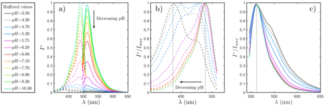
2.17 Spectral band intensities and ratio as a function of pH measured by spectroflu-orimetry . . . 66
LIST OF FIGURES
2.18 Sketch of the setup designed for the turbulent jet experiment . . . 67
2.19 Calibration images at homogeneous pH = 7 . . . 68
2.20 Measured ratio as a function of pH. . . 68
2.21 Evolution of fluoresced light intensity and ratio with laser power output . . . . 70
2.22 Effect of fluorescence re-absorption . . . 70
2.23 Comparison of instantaneous pH field obtained by single or two-color IpH−PLIF 71 2.24 Effect of laser power drift on IpH− PLIF and IrpH− PLIF . . . 72
2.25 Evolution of acid concentration along the jet centerline . . . 73
2.26 Jet characteristics - Transverse profiles . . . 73
2.27 Influence of XG concentration on excitation and fluorescence spectra of fluo-rescein . . . 75
2.28 R = f (pH) calibration curves for water and dilute XG solutions . . . 76
2.29 Diphasic test case for IrpH− PLIF . . . 76
2.30 IpH− PLIF noise related errors . . . 77
2.31 Relative uncertainty mapping of ratio as a function of measured spectral band intensitiesδI1andδI2. . . 78
2.32 Effect of pH on ratio uncertainty and of ratio uncertainty on pH and concen-tration measurement . . . 80
3.1 Fluid energy spectrum for viscoelastic turbulence . . . 89
3.2 Illustration of a flow cavern in a stirred tank by Xiao et al. (2014) . . . 92
3.3 Non-exhaustive collection of XG viscosity curves found in the litterature . . . . 98
3.4 Measured pH of XG dissolved into distilled water as a function of polymer con-centration . . . 101
3.5 Viscosity versus shear rate curves for XG solutions in distilled water at different concentrations . . . 102
3.6 Evolution of characteristic solution time scale and zero shear rate viscosity with XG concentration in salt free solutions . . . 103
3.7 Storage/elastic and loss/viscous moduli G0and G" as a function of oscillations frequency and XG concentration . . . 104
3.8 Surface tension measurements and litterature data for XG solutions . . . 104
3.9 Tank and grid design . . . 105
3.10 Evidence of polymer stability to the grid’s oscillations . . . 108
3.11 Regions of interest and of calculation for close grid and full tank experiments . 109 3.12 Setup for PIV study of OGT . . . 109
3.13 Grid masking procedure . . . 111
3.14 Grid tracking procedure . . . 111
3.15 Graph of convergence of statistical quantities . . . 114
3.16 Mean flow inside the grid stirred tank at different XG concentrations: 2D norm 115 3.17 Streamlines of the mean flow inside the grid stirred tank at different XG con-centrations. The region of measurement and scales are the same than figure 3.16. . . 116
3.18 Mean flow inside the grid stirred tank at different XG concentrations: vorticity . 117 3.19 Evolution of maximum vorticity associated to mean flow structures as a func-tion of polymer concentrafunc-tion . . . 119
3.20 Effect of polymer concentration on vertical velocity. . . 120
3.21 Example of close grid instantaneous velocity and vorticity fields . . . 123
3.22 Average, phase average, oscillating and fluctuating velocity and vorticity fields for water and 100 ppm DPS . . . 124
3.23 Oscillating vorticity field at different grid positions in the close grid region for
water and DPS . . . 125
3.24 RMS of turbulent fluctuations at different grid positions in the close grid region for water . . . 126
3.25 RMS of turbulent fluctuations at different grid positions in the close grid region for 100 ppm XG solution . . . 127
3.26 RMS of oscillatory and turbulent velocity fluctuations . . . 129
3.27 Reynolds stresses in water and DPS . . . 130
3.28 Oscillatory stresses u∗iu∗j fields induced by the periodic velocity fluctuations. . 131
3.29 Triple decomposition transfer terms in water and DPS . . . 132
3.30 Vertical profiles of oscillatory and Reynolds normal stress and transfer terms for water and DPS. . . 134
3.31 Local statistics of apparent viscosity . . . 135
3.32 Example of phase averaged viscosity fields at different grid positions . . . 135
3.33 Turbulent kinetic energy fields for water and DPS at different concentrations . 137 3.34 Hopfinger and Toly’s type profiles of the rms of horizontal and vertical turbu-lent velocity fluctuations . . . 138
3.35 Vertical profiles of isotropy and horizontal homogeneity for water and DPS so-lutions at different concentrations . . . 139
3.36 Fields of mean flow over turbulence ratio in water and DPS . . . 141
3.37 Example of correlation coefficients as a function of Z for 50 ppm XG solution . 142 3.38 Integral length scales of OGT in water and DPS . . . 143
4.1 Sketch of the characteristic hydrodynamic sub-layers of near surface turbulence153 4.2 Main principles of turbulent mass transfer at a flat interface. . . 154
4.3 Sketch of the characteristic scalar sub layers of near surface turbulence . . . 156
4.4 Full experimental setup for SPIV and PLIF coupled measurements . . . 168
4.5 Experimental pH-CO2curves in XG solutions . . . 171
4.6 Example of IrpH− PLIF calibration curves and fitting constants . . . 173
4.7 Example of IrpH− PLIF calibration procedure . . . 174
4.8 Binning options . . . 176
4.9 Schematic representation of the timming of PLIF and PIV synchronisation . . . 176
4.10 Depths and ROI for coupled measurements . . . 176
4.11 Mean flow under the gas-liquid interface for water and DPS at different con-centrations . . . 183
4.12 Mean to turbulence ratioΓunder the gas-liquid interface for water and DPS at different concentrations . . . 185
4.13 Example of instantaneous u0fields . . . 187
4.14 Sub-surface profiles of rms velocities and turbulent intensity . . . 188
4.15 Sub-surface rms profiles of horizontal velocity fluctuations and evolution of the viscous sub-layer depth with polymer concentration . . . 192
4.16 Evolution ofδv/δµv0with the Deborah number in the very dilute range . . . 194
4.17 Sub-surface profiles of rms of velocity fluctuations scaled by their value at the viscous sub-layer depth . . . 195
4.18 Vertical gradient of vertical velocity fluctuations and quantification of the sur-face oscillations . . . 197
4.19 PDF of velocity fluctuations for water and DPS at three relative depths . . . 200
4.20 Conditional analysis of the Reynolds stresses in water and DPS . . . 201
LIST OF FIGURES
4.22 Sub-surface integral velocity length scales . . . 206
4.23 Instantaneous dissolved CO2concentration fields in water . . . 211
4.24 Instantaneous dissolved CO2concentration fields in water and DPS . . . 212
4.25 Time series of x averaged instantaneous concentration for water and 10 ppm DPS at two different depths . . . 214
4.26 Average concentration profiles at different times obtained by fitting of concen-tration time series at each depth . . . 214
4.27 Time series of bulk and apparent surface concentration estimated by exponen-tial fitting of average concentration profiles . . . 216
4.28 Time series of x averaged concentration fluctuations for water and 10 ppm DPS at two different depths . . . 216
4.29 PDF of concentration fluctuations . . . 217
4.30 Two point concentration correlation coefficient and concentration fluctua-tions integral length scale for WD and XG10A runs . . . 218
4.31 Two times concentration correlation coefficient and concentration fluctua-tions integral time scale for WD and XG10A runs . . . 219
4.32 Coupled instantaneous velocity and dissolved gas concentration fields in water 223 4.33 Coupled instantaneous velocity and dissolved gas concentration fields in 10 ppm DPS . . . 224
4.34 Coupled fluctuating velocity and dissolved gas concentration fields in water . . 225
4.35 Coupled fluctuating velocity and dissolved gas concentration fields in 10 ppm DPS . . . 226
4.36 Width averaged profiles of u0ic0correlations and their rms for water and DPS . . 227
4.37 Joint PDF of u0zand c0for water and DPS . . . 228
4.38 Covariance integrand of u0zand c0for water and DPS, small amplitude concen-tration fluctuations . . . 229
4.39 Covariance integrand of u0zand c0for water and DPS, large amplitude concen-tration fluctuations . . . 230
4.40 Probability profile of each hexadecan in water and DPS . . . 230
4.41 Probability profile of each quadrant in water and DPS . . . 231
4.42 Quadrant sorted vertical turbulent mass fluxes u0zc0as a function of depth . . . 232
4.43 Global mass transfer for the WD and XG10A runs . . . 235
4.44 Global mass transfer velocities KLestimated from bottom tank pH measurements235 4.45 An insight on 3D3C measurements in 25 ppm DPS using LaVision MiniShaker cameras and the Shake the box algorithm. . . 243
B.1 Computer aided design of the oscillating grid setup . . . 266
B.2 Kinematic diagram of the oscillation system . . . 267
B.3 Normalized position, velocity and acceleration of the grid, along with its veloc-ity spectrum normalized by its maximum value . . . 268
C.1 Example of POD modes . . . 271
C.2 POD eigenvalue spectrum . . . 273
C.3 Cumulative energy contained in the POD modes . . . 273
C.4 POD eigenvalue spectrum of dilute polymer solution normalized by the water spectrum for the three regions of the flow. . . 274
C.5 θi coefficients as a function of the instantaneous field index. . . 275
C.6 Histogram plot ofθi coefficient values. . . 276
C.7 2D and 3D scatter plots ofθ coefficients. . . 277
C.8 Comparison between oscillatory velocity fields obtained using phase averaged measurements and and POD reconstruction . . . 279
C.9 Reconstructed rms profiles . . . 281
D.1 Experimental setup for pH-CO2curves measurement in presence of different additives . . . 284
D.2 Experimental results of fluorescein’s effect on pH-CO2equilibria . . . 285 D.3 Chemical species production during CO2bubbling of fluorescein sodium
solu-tions and possible surfactant production mechanism . . . 286
D.4 Effect of buffered pH on XG flow curves . . . 288
D.5 Relative variations of zero shear rate viscosity in presence of acidic and basic salts with respect to its value for XG solutions in distilled water . . . 288
D.6 Effects of CO2dissolution on the rheology of XG . . . 289 F.1 Horizontal scalar structures observed by qualitative fluoresced light intensity
recording . . . 293
G.1 Calibration curves for single color methods S and Sa, and for the ratiometric method . . . 297
G.2 Correction of the outer region absorption based on ratiometric measurement of C(z, t ). . . . 298
G.3 Comparison of pH and C fields obtained by R, S and Sa methods. . . 299
G.4 Local and width averaged concentration profiles along depth, obtained by R, S or Sa method. . . 300
List of Tables
2.1 Extinction coefficient values atλ = 491 nm from Klonis and Sawyer (1996) . . . 58
2.2 Wavelengths used for the present spectral study . . . 63
3.1 Some applications of XG and typical concentrations used . . . 96
3.2 Parameters for PIV study of OGT . . . 110
3.3 Evolution of maximum vorticity associated to mean flow structures as a func-tion of polymer concentrafunc-tion in the dilute range . . . 118
3.4 Slopes of the linear part of integral length scales profiles versus depth in water and DPS . . . 142
4.1 Literature overview on turbulent mass transfer, non-Newtonian effects and gas-liquid interfaces . . . 163
4.2 Table of characteristic undisturbed velocity and length scale variations with polymer concentration through the experimental runs of the dissolution study 167
4.3 Table of dimensionless parameters variations with polymer concentration through the experimental runs of the dissolution study . . . 167
4.4 Recap of the experimental runs for near surface turbulence and dissolution study178
4.5 Definition of quadrants and hexadecants for conditional analysis of Reynolds stresses and turbulent mass fluxes . . . 181
4.6 Table of characteristic velocity and length scales at z=δv . . . 207
Abbreviations
DIC Dissolved Inorganic Carbon dioxide
I − PLIF Inhibited Planar Laser Induced Flu-orescence
IrpH− PLIF Ratiometric, pH sensitive Inhib-ited Planar Laser Induced Fluores-cence
IrT− PLIF Ratiometric, temperature sensitive Inhibited Planar Laser Induced Fluo-rescence
IO2− PLIF Inhibited Planar Laser Induced
Fluorescence for dissolved oxygen concentration measurement
IpH− PLIF pH sensitive Inhibited Planar Laser Induced Fluorescence
IT− PLIF Temperature sensitive Inhibited
Planar Laser Induced Fluorescence 2D2C Two dimensions, two components 2D3C Two dimensions, three components BJ Related to Brumley and Jirka (1987)
CG Close Grid region
CWL Continuous Wave Laser CY Carreau-Yasuda (fitting, law...)
DNS Direct Numerical Simulation
DPS Dilute polymer solution
DR Drag Reduction
FT Full Tank
GN Grid neighborhood region
HIT Homogeneous Isotropic Turbulence
HT Related to Hopfinger and Toly (1976)
HXi Hexadecan i
LES Large Eddy Simulation
LIF Laser Induced Fluorescence
MCFD Multiphase Computational Fluid Dy-namics
Nd:YAG Neodymium-doped Yttrium Alu-minium Garnet (laser)
OGT Oscillating Grid Turbulence PDF Probability Density Function
PEO Poly-Ethylene Oxide
PIV Particle Image Velocimetry
PLIF Planar Laser Induced Fluorescence POD Proper Orthogonal Decomposition PTV Particle Tracking Velocimetry
Qi Quadrant i
RANS Reynolds Averaged Navier Stokes Equations
RASJA Random Array of Synthetic Jets Actu-ators (Variano and Cowen,2013) SPIV Stereoscopic Particle Image
Velocime-try
SZ (Grid) Sweep Zone region
TKE Turbulent Kinetic Energy
TT Related to Thompson and Turner
(1975)
XG Xanthan gum
Chemistry
[.] Molar concentration
Fl Fluorescein sodium (all forms
NOMENCLATURE
Fl+ Cationic forms of fluorescein sodium
Fl− Mono-anionic forms of fluorescein
sodium
Fln Neutral forms of fluorescein sodium
Fl2− Dianionic forms of fluorescein
sodium
H2CO3 Carbonic acid
H2CO∗3 Apparent carbonic acid (carbonic
acid plus aqueous carbon dioxide NaOH Sodium hydroxide
CO2 Carbon dioxide
CO2−3 Carbonate ion
HCO−3 Hydrogen carbonate ion
O2 Di-oxygen Dimensionless numbers Ca Capillary number De Deborah number Fr Froude number Ha Hatta number Re Reynolds number
Reg Grid Reynolds number
ReT Turbulent Reynolds number
Reλ Reynolds number based on the Taylor
microscale
Sc Schmidt number
St PIV particles Stokes number
Wi Weissenberg number
Statistics and operations
〈a〉φ,r ms Phase rms of a
〈a〉φ Phase average of a
〈a〉r ms Root mean square (rms) value of a [a]X Average of field a along dimension X
[a]r ms,X RMS of field a along dimension X a · b Dot product of a and b
∇ Gradient (nabla) operator
⊗ Tensor product
a Statistical average of a
a0 Turbulent fluctuation of a
a∗ Oscillatory/periodic fluctuation of a P(a,b) Joint probability of variables a and b
Symbols
α Scheimpflung angle
β Instantaneous surface divergence
˙
γ Shear rate tensor
νT Eddy viscosity tensor
σ Cauchy stress tensor
τ Shear stress tensor
δI1 Intensity collected from spectral band
1
δI2 Intensity collected from spectral band
2
∆S Grid stroke sampling definition
∆t PIV time interval
δB Batchelor sub-layer
δD Apparent diffusive film thickness
δ(ap p)D (Apparent) diffusive sub-layer δO Outer diffusive sub-layer
δv Viscous sub-layer
δη Kolmogorov sub-layer
² Fluorescein molar extinction
coeffi-cient (I-PLIF)
² Turbulent dissipation rate
η Kolmogorov length scale
ηB Batchelor scale
Γ Mean to turbulence ratio
κ Wave number
λe Laser excitation wavelength
λf (fluorescence) Wavelength
λk
i j Taylor micro scale for components i and j in dimension k
g Gravity
I Identity matrix
U Liquid phase instantaneous velocity
Tmo Mean flow to oscillatory motion en-ergy transfer term
Tot Oscillatory motion to turbulence en-ergy transfer term
µ Dynamic viscosity
µ0 Zero shear rate viscosity
µ∞ Infinite shear rate viscosity
µap p Apparent (approximated) viscosity
ν Kinematic viscosity
Ω Out-of-plane vorticity
φ Fluorescence quantum yield (I-PLIF)
ρ Density
ρp PIV particles density
σ Surface tension
θ Stereoscopic PIV angle
Ξ Grid solidity parameter
A Optical constant
a Newtonian to non-Newtonian
transi-tion parameter
C Fluorescent dye concentration
Cki Concentration of species i in phase k Ckb,i Bulk concentration of species i in
phase k
Cksat ,i Saturation concentration of species i in phase k
Cb ROI bulk concentration
Cs Measured surface concentration
C1HT Hopfinger and Toly’s constant for u0x C2HT Hopfinger and Toly’s constant for u0z
Cbt Bottom tank dissolved gas concentra-tion
Csat Saturation concentration defined by Henry’s law
CTT Thompson and Turner’s constant
CXG Xanthan gum concentration
d Grid bar size
Di Molecular diffusion coefficient of
species i in water
d Ia Local absorbed intensity
d If Local fluoresced light intensity
d t Camera’s exposure time
eL Laser sheet thickness
f Grid oscillations frequency
f Lens focal length
fac q Acquisition frequency
G Elastic modulus
G0 Storage/elastic modulus
G00 Dissipation/loss modulus
Hij Homogeneity index of component j
along dimension i
HG Average grid - bottom distance
HS Average grid - surface distance
Hc,i Henry constant of species i Ht ot Total fluid height in the tank I0 Laser output intensity
If Fluoresced intensity
Ii Incident intensity
Ir Received fluoresced light intensity Ii js Isotropy indicator in dimensions i,j
k Turbulent kinetic energy
Ka Reaction constant of hydrogen
car-bonate production
Kb Reaction constant of carbonate
pro-duction
kg Gas side gas-liquid mass transfer co-efficient
Kh Reaction constant of carbonic acid
production
kL Liquid side gas-liquid mass transfer
coefficient
Ls Length of fluid sample crossed by the incident beam
L∞ Bulk integral length scale of turbu-lence
Lki j ,α α percent integral length scale for components i and j in dimension k
NOMENCLATURE
Lki j Integral length scale for components i and j in dimension k
Lobs Distance between a point in the fluid and the sensor
M Grid mesh parameter
mki Mass of species i in phase k
nx Exponent of the Hopfinger and Toly’s
decay law for u0r ms
Np Number of slices for the grid stroke
sampling
p liquid phase pressure
pi∗ Partial pressure of species i
R Spectral bands ratio
R∗ Wavelengths ratio
Rn Normalized intensity ratio Rr Ratio submitted to re-absorption Rki j Correlation coefficient of components
i and j in dimension k
S Grid oscillations amplitude/stroke
Sφ Spectral quantum yield
sp x Surface of the laser sheet correspond-ing to one camera pixel
T Characteristic deformation time
Tc Integral concentration time scale
tc Characteristic relaxation time of a ma-terial/solution
tD Typical time scale of diffusion
Tg Gas phase temperature
Vk Volume of phase k
Zh Horizontal homogeneity limit for os-cillating grid turbulence
KL Total gas-liquid mass transfer
coeffi-cient
tCY Characteristic polymer time scale
All life is an experiment. The more experiments you make the better.
Ralph Waldo Emerson
The study of mass transfer at the interface between a gas and a liquid is of great interest in many environmental phenomena and industrial processes. In the industry, the physics of mass transfer defines the efficiency of diphasic mixing and degassing in stirred tanks, bubble columns, or even more complex mixing tank geometries. As an example, in photobioreactors for micro-algae production, gaseous carbon dioxide CO2has to be dissolved into the culture
waters to be then consumed through photosynthesis. Optimizing micro-alga production re-quires a better understanding and modelling of this CO2dissolution so that the mass transfer
rate from gaseous to aqueous phase can be predicted and maximized (Valiorgue et al.,2014). From an environmental point of view, the same mechanisms also control the dissolution of atmospheric gases into the oceans, rivers and lakes, and have therefore a huge impact on cli-mate and biodiversity. Even though this issue has already been studied for several decades, its understanding is still not good enough to create realistic models suitable for implemen-tation in Multiphase Compuimplemen-tational Fluid Dynamics (MCFD) codes. The difficulty in depict-ing such phenomena lies in the fact that they depend on numerous factors, among which, the diffusivity of transported species, the shape and dynamics of the interface, the charac-teristics of turbulence in each phase, the presence of chemical reactions, microorganisms, photocatalysis, and the possibly complex rheology of the liquid side.
Due to its strong ability in passive scalar mixing, turbulence is one of the main con-tributors to the efficiency of mass transfer. Its action is nevertheless quite complex, and it can have multiple effects in the full process. For example turbulence may both acceler-ate the growth of micro-organism by enhancing carbon dioxide dissolution into the culture medium, or reduce it by destroying cell clusters (San et al.,2017). In fermentation broths, the development of bacteria is powered by gas dissolution and turbulence. Yet this development causes the transition of the liquid phase from a Newtonian low viscosity to a high viscosity shear-thinning behavior, which itself tends to reduce mass transfer efficiency (Gabelle et al.,
2011).
The part played by turbulence in gas-liquid mass transfer has been the subject of a huge amount of work for almost a century (Lewis and Whitman (1924) to Wissink et al. (2017)), but the exact mechanisms of mass transfer turbulent enhancement still remain unclear. Several investigations have been made using numerical simulations, channel flows, or stirred tank experiments (Herlina and Wissink, 2014; Turney and Banerjee, 2013; Variano and Cowen,
2013). Because of their environmental applications, most of these studies focused on dis-solution of atmospheric gas into water, considered to be slow diffusion species. All studies
INTRODUCTION
involving atmospheric gases and large Reynolds numbers on the liquid-side with respect to the one on the gas side agree on the fact that the influence of the interface on liquid-side turbulence is significant at very small depth of the order of 1 cm. The main challenge of current works is to achieve sufficient spatial resolution of simulations or experimental ob-servations in order to describe the mass transfer phenomenon inside those small interfacial layers. Such a spatial resolution is nowadays achievable numerically thanks to the improve-ment of computational power allowing the use of direct numerical simulation (DNS) at small scales (Herlina and Wissink,2014; Wissink et al.,2017). Experimentally, a wide range of opti-cal techniques, boosted by growing data processing capacity, can be used to access instanta-neous, multi-point and information of many properties of the flow: velocity, pressure, scalar field concentration (as in figure2)...
Figure 2 – Example of three instantaneous dissolved gas fields obtained by fluorescence imaging. White color represent the null dissolved gas concentration, green intermediate concentrations and black high concentrations (in arbitrary unit). Each picture is 19 mm wide along the horizontal dimen-sion, and 16 mm along the vertical (depth). The gray rectangle denotes the gaseous phase saturated with CO2.
While the understanding of turbulent gas-liquid mass transfer in water and more gen-erally Newtonian fluids has improved in the last decades, the influence of the fluid’s com-plex aspect and non-Newtonian behavior on fundamental principles of turbulent gas-liquid mass transfer remain unknown. The behavior of such fluids being very different from that of Newtonian liquids, specific features due to shear thinning or viscoelastic behaviors appear industrial processes (Gabelle et al.,2011; Xiao et al.,2014). Efficient models for Newtonian fluids fail at predicting mass transfer in non-Newtonian fluids. Despite the apparent inter-est for many industrial applications, the literature still lacks fundamental experiments and simulations to describe non-Newtonian turbulent mass transfer. Such studies have the same spatial resolution issues than experimentation in water with additional complexity brought by the coupling between polymer chains and turbulence.
One of the most popular experimental setups to study turbulence alone without any strong mean flow and its effects on mass transfer at a free surface is the oscillating grid system. Oscillating grid turbulence (OGT) has been used from more than 40 years and is still used nowadays (Hopfinger and Toly, 1976; Thompson and Turner, 1975) to study fundamental aspects of turbulence near solid boundaries (McCorquodale and Munro,
2018), in stratified media (Verso et al.,2017), and at gas-liquid interfaces (Brumley and Jirka,
1987; Chiapponi et al.,2012), or its action on dispersed phases of cells or fibers (Cuthbertson et al., 2018; Mahamod et al.,2017; Nagami and Saito,2013; Rastello et al.,2017; San et al.,
2017). Yet OGT has been used with non-Newtonian media only in a few studies (Liberzon et al.,2009; Wang et al.,2016), and never in a two phase configuration.
questions:
• How can non intrusive optical techniques be improved in order to get useful data at the small scales of turbulent mass transfer ?
• How does oscillating grid turbulence (OGT), long time studied in water, behave in complex polymer solutions; and how can we use the OGT tool to generate controlled turbulence in such fluids?
• What are the effects of complex rheological properties, in particular those of dilute polymer solutions, on near surface hydrodynamics, turbulent mixing, and mass trans-fer mechanisms at gas-liquid interfaces ?
With the aim of bringing part of the answers to those key questions, this work is focused on the case study of a well known gas: carbon dioxide. Optical metrology is developed and implemented in order to document its dissolution and turbulent mass transfer. Complex fluids are here modeled by shear thinning viscoelastic solutions of Xanthan Gum (XG). An oscillating grid system is designed for the study of turbulent gas-liquid mass transfer, and its behavior tested in non-Newtonian solutions. Turbulent gas-liquid mass transfer is finally addressed in simplified and fundamental conditions: at a flat interface with only liquid side bottom shear turbulence generated by an oscillating grid.
In this context, the manuscript is structured as follows. The first chapter is an introduc-tion to the main concepts and phenomena studied in this thesis, namely gas-liquid mass transfer, turbulence and its mixing efficiency, and non-Newtonian fluids. The second chap-ter presents the two main experimental techniques employed throughout this thesis. A sig-nificant part of the chapter is dedicated to the development and improvement of the flu-orescence based method used for dissolved gas concentration measurement. In the third chapter, results of an experimental study of OGT in water and dilute polymer solution are detailed. This chapter is also used to introduce and characterize XG. The last chapter details the experimental observations of carbon dioxide dissolution into water and aqueous XG so-lutions at a flat interface and under the action of OGT. As a conclusion, the main results exposed in the previous chapters are summarized, and perspectives and guidelines of future works are discussed.
Chapter
1
Definitions
It is better to know some of the questions than all of the answers
James Thurber
Contents
1.1 Gas-liquid mass transfer. . . . 6 1.1.1 Main principles . . . 6
1.1.2 Global mass flux and mass transfer coefficient. . . 8
1.1.3 Examples. . . 11
1.2 Turbulence . . . 12 1.2.1 General definitions . . . 13
1.2.2 Turbulence and mixing . . . 21
1.3 Non-Newtonian fluids . . . 25 1.3.1 Non-Newtonian behaviors . . . 25
This chapter provides an introduction to the main concepts and phenomena stud-ied in this thesis. It starts with a defini-tion of gas-liquid mass transfer and a pres-netation of its main applications. Mass transfer from a gaseous phase towards a liquid one finds is ruled by Henry’s law, which determines the equilibrium concen-tration ultimately reached by each phase. The speed at which transfer occurs de-pends on many parameters, among which the nature and shape of the interface, the aerodynamics of the gaseous phase, or in our focus, the hydrodynamics of the liquid phase. More specifically, liquid side tur-bulence enhances mass transfer in many environmental an industrial applications. Turbulence should then be defined, and this is done in the second part of the chap-ter. To do so, the governing equations of hydrodynamics and mass transport are ex-pressed, and their stochastic version used for turbulent flow description are detailed. Characteristic quantities of turbulence and turbulent mixing are also defined. The last part of this chapter consists in a descrip-tion and a definidescrip-tion of non-Newtonian fluids. The behavior of turbulence within those fluids is even more complex than the Newtonian case. Constitutive equations, modified governing equations, and spe-cific quantities are introduced to try and describe it.
Ce chapitre sert d’introduction aux prin-cipaux concepts et phénomènes étudiés
au cours de cette thèse. Il débute par
une définition du transfert de masse gaz-liquide et une présentation de ses applica-tions. Le transfert de masse d’une phase gazeuse vers une phase liquide trouve son origine dans la loi de Henry qui déter-mine la concentration d’équilibre entre les deux phases. La vitesse à laquelle se produit le transfert dépend de nombreux paramètres, parmi lesquels, la nature et la forme de l’interface l’aérodynamique de la phase gazeuse, ou encore celui qui nous intéresse dans cette thèse : l’hydrodynamique de la phase liquide. En particulier, la turbulence en phase liq-uide accélère le transfert de masse dans le cadre de nombreuses applications en-vironnementales ou industrielles. Il con-vient donc de définir la turbulence, ce qui est fait dans une seconde partie. Pour ce faire les équations fondamentales de l’hydrodynamique et du transport de matière dans les fluides sont introduites, et leur version stochastique permettant de décrire les écoulements turbulents est présentée. Les grandeurs caractéristiques de la turbulence et du mélange en phase liquide sont finalement introduites. Enfin, la dernière partie de ce chapitre propose une description et une définition de ce que sont les fluides non Newtoniens. Présents dans de nombreuses applications, le com-portement de la turbulence au sein de ces fluides est grandement complexifié par rapport au cas newtonien. Divers modèles de comportement, équations modifiées, et grandeurs spécifiques sont proposées pour tenter de décrire au mieux ces comporte-ments.
CHAPTER 1. DEFINITIONS
This chapter provides introduction to the main concepts that will be used in the rest of the manuscript. Gas-liquid mass transfer, turbulence, and non-Newtonian fluids are intro-duced. The term of mass transfer is first defined, and physical phenomena governing mass transfer between a gaseous and a liquid phase are explained. Some common examples of gas-liquid mass transfer situations are also described. The second section starts with a brief introduction to turbulent flows and their governing equations and scaling. The effect of tur-bulence on passive scalar mixing in fluid flows is then discussed. In the last section, the non-Newtonian nature of a fluid is defined, and a brief review of existing non-Newtonian behaviors and their industrial, environmental, biological or every-day life applications is presented. Finally, relevant dimensionless numbers and governing equations for the de-scription of non-Newtonian flows are defined.
In particular, non-Newtonian and turbulence-related definitions are later used in chapter 3 for the study of turbulence in shear thinning and viscoelastic dilute polymer solutions (DPS). Mass transfer physics is then added in chapter4to discuss gas dissolution at a flat gas-liquid interface in Newtonian or non-Newtonian media.
1.1 Gas-liquid mass transfer
In this section, the main principles of mass transfer are defined, and in particular those of mass transfer between a gaseous and a liquid phase. The concepts explained in the first paragraph are used to define a global approach to mass transfer measurements in a second paragraph, and illustrated by concrete industrial and environmental examples in the last paragraph.
1.1.1 Main principles
Mass transfer of a given species between two phasesφ1andφ2is defined as the exchange of
part or all the mass of this species from one phase to the other. This exchange is based on a thermodynamic transformation, chemical reaction, or both, allowing part of the species to change phase. One may distinguish between changes of state, which are purely thermo-dynamical processes involving one single species (e.g water boiling or condensation), and mass transfer between phases, which can be a combination of thermodynamical and chem-ical reactions and often involve two or more species (e.g. dissolution of salt into water). Depending on the two phases involved and the physics of the mass transfer, different names may be used (see figure1.1).
In real life situations, many phases may be present at the same time, each of which con-taining several chemical species. Rivers and water ways and their interfaces with both at-mospheric gases and bottom solid sediments, or industrial bubble columns reactors with solid catalyst particles are two good examples of how complex multiphase mass transfer sit-uations can be.
All mass transfer problems are ruled by the mass conservation principle, which states that the total mass of a given element over all phases remains constant between the initial and the final states. Dealing with chemical reactions, one as to keep in mind that the conserved mass is not necessarily that of the chemical species, but the mass of chemical elements. A general mass conservation equation for species i in phase k of a system of N phases could be written as d mik d t =P k i − C k i + N X p=1 Jip−→k (1.1)
Figure 1.1 – Names of two phases mass transfer involving a single (change of state) or several species (mass transfer)
.
WherePik andCikare respectively the rates of production and consumption of species i in phase k, due for example to chemical reactions occurring in this phase; andJip−→k is the mass flux of species i from phase p to k. For a system with only two phases exchanging a single species i , and no production or consumption terms, this equation simplifies to:
d mi1 d t =J 2−→1 i = −Ji1−→2= − d m2i d t (1.2)
Similar equations can be derived for the concentration Cikof species i in phase k. Cikis the intensive quantity corresponding to mass, which is extensive1
d C1i d t + ∇ j
2−→1
i = 0 (1.3)
where ∇ is the gradient operator. This equation is the general governing equation for passive scalar transport. As defined above, the mass flux ji2−→1is the net quantity of the considered species transferred from phase 2 to 1 in a time increment dt, per surface unit. This local mass flux is a function of the local gradient of concentration: if a concentration gradient exists, diffusion occurs in order to balance that gradient.
Diffusion is the displacement of species in a fluid induced by molecular dynamics. It is characterized by the molecular diffusion coefficient of species i in phase 1 D1i in m2/s. The greater the diffusion coefficient, the faster a species "moves" across a fluid at rest. According to Stokes-Einstein relationship, the diffusion coefficient of a species i in a solvent k scales as
Dki ∼ θ
rµ (1.4)
where θ is the temperature, µ the dynamic viscosity and r the apparent radius of the molecule being diffused. For a given species, the diffusion coefficient thus increases with increasing temperature or decreasing viscosity. The previous relationship is valid for large molecules moving through Newtonian solvents under Brownian motion.
Fick’s second law of diffusion assumes the local mass flux to be proportional to the local concentration gradient such that ji2−→1= D1i∇Ci1(Fick,1855). Other mechanisms can also be responsible of component motion in the fluid (electrical, magnetical, hydodynamic...). The
1Intensive quantities are quantities for which the magnitude does not depend on the size of the system, for
example temperature or pressure. Extensive quantities are quantities for which are directly proportional to the amount of matter present in the system, for example the number of moles, volume, flow rate. Homogeneous systems are defined as systems where intensive quantities have the same value at all points.
CHAPTER 1. DEFINITIONS
most common one is of course the motion of the fluid itself. Transport of species by fluid motion is called convection or advection2. One of the hardest challenges in mass transfer studies is to account for the effect of advection in complex situations and complex fluids. Most of the time, the interactions between fluid motion and diffusion process at the interface are not well understood, mainly because the regions in which mass transfer occurs is beyond the spatial resolution capacity of many experimental methods and numerical simulations.
In the following sections, emphasis is given to gas-liquid mass transfer situations. How-ever, most of the concept discussed remain valid for many other two phase mass transfer situations. We consider hereinafter the case a source gaseous phaseφ2transferring mass to
a liquid phaseφ1.
1.1.2 Global mass flux and mass transfer coefficient
Most of the mass transfer studies do not focus on local aspects but rather on estimating a global evolution of C1i in the receptive fluid phase. The key parameter to estimate is then the global mass flux at the interface, which is generally written as :
ji2−→1=KL
L ∇C
1
i (1.5)
Where L is a typical length of transfer. The global mass balance equation for the φ1toφ2
mass transfer is then:
∂C1i
∂t = KL a
V1
∇2C1i (1.6)
with L = V1/a. The speed of a mass transfer process is thus conditioned by three main factors:
• the surface of exchanges a, and more specifically the ratio between this surface area and the volume of the receptive phase V1.3
• the gradient of species ∇Ci1. It can be related to the tension at the interface∆C1i = Ci ,sat1 − C1i ,b, which is the difference between the "bulk" (far from the interface) con-centration C1b,i of i in phaseφ1at a given time, and the concentration C1sat ,i for which
the two phases would be at equilibrium.
• the mass transfer coefficient/velocity of species i from 1 to 2, which depends itself on the physical and chemical mechanisms involved in mass transfer
1.1.2.a Surface of exchanges and interface gradient
For a constant V1, the larger the surface, the faster the global transfer. Mass transfer is all
the more efficient when the interfacial area is maximized with respect to the volume of the receptive phase. This one of the reasons for which mass transfer around bubbles at a given rise velocity is more efficient for a large number of small bubble than for fewer larger
2Here the term advection is preferably used in order to avoid confusion with heat transfer
3Note that a does not appear in equation (1.3) since it is a local mass transfer equation, but that the total
mass flux in a global configuration is an integration of the mass flux per unit surface over the total surface of exchanges.
bubbles4.
When a gaseous and a liquid phase are in contact at an interface, the saturation value Csat ,i in the liquid phase is fixed by the partial pressure of the same species in the gaseous phase pi∗according to Henry’s law5(Henry,1803):
p∗i = Hc,iCsat ,i (1.7)
Where Hc,i is a constant fixed by the gas-liquid couple used and by temperature. ∆C = C1sat ,i− Ci1powers mass transfer until the saturation value Csat ,i is reached at every point of the volume of fluid.
1.1.2.b Mass transfer coefficient
The mass transfer coefficient KL is the major parameter used to estimate the efficiency of
mass transfer, which depends on many factors. The main ones are diffusion properties of the dissolved gas, chemical reactions involving transferred species, and hydrodynamics of the liquid phase.
For a gas-liquid interface where only diffusion occurs, Lewis and Whitman (1924) showed that the mass transfer coefficient may be decomposed as a series association of two mass transfer velocities, one on the liquid side kLand one on the gas side kg:
1 KL = 1 kL +RTgHc kg (1.8) With R = 8.314 J.K−1.mol−1the ideal gas constant, and Tg the gas temperature. The inverse of mass transfer velocities evaluate resistance to mass transfer: 1/KLis the equivalent
resis-tance to mass transfer of two resisresis-tances in series, the liquid side one and the gas side one. For poorly soluble gases such as oxygen, nitrogen, or carbon dioxide, Henry’s law constant Hc is about Hc ∼ 10−4 mol.m−3.Pa−1 and kg >> kL. This implies that
RTgHc
kg , the gas side resistance, is weak, and that KL∼ kL.
With that picture, the mass flux going from the gaseous to the liquid phase is equal to the mass flux crossing the diffusive film. In other words, the concentration profile is linear in the diffusive layer (see figure1.2) and the mass transfer coefficient is (Lewis and Whitman,
1924): KL= Di δD (1.9) whereδD= ∆C1i ∇i ntC1i
is the diffusive film thickness, deduced from the concentration gradient at the interface ∇i ntC1i. The thinner the diffusive film, the larger the mass transfer veloc-ity. Effects of advection on mass transfer can now quite easily be understood: by removing saturated fluid from the interface or by mixing efficiently the receptive phase, the thickness of the liquid film can be reduced and strong concentration gradients can be maintained at
4In reality, the question of mass transfer around bubbles is more complex since it also involves advection
at the interface, which depends on the bubble rise velocity. This bubble rise velocity increases with buoyancy effects, and so with the bubble size
5This writing of Henry’s law assumes that the thermodynamical activity coefficient of the dissolved gasγ
i
and its fugacity coefficientφi are both equal to unity These assumptions are valid in thermodynamically ideal
solutions, for which concentrations of salt and dissolved species are small, which is assumed to be the case here.
CHAPTER 1. DEFINITIONS
Figure 1.2 – Concept of the diffusion film in gas-liquid mass transfer
the interface, thus improving the diffusion efficiency. For example, the rising of bubbles in water due to buoyancy effects allows for the replacement of saturated fluid in the vicinity of the interface and to efficient mass transfer (Valiorgue et al.,2013; Vega-Martínez et al.,2017). As for bulk mixing, one of the most efficient process in that matter is without doubt turbu-lence. The reasons for this efficiency are explained in section1.2.2. Fluid motion impact on the estimation of mass transfer coefficient is complex, and therefore many different models and empirical correlations exist depending on the type of flow and on the type of interface. It is worth noting that advection in the gaseous phase has the same effect on kg, and thus on KLfor more soluble gases or in situations where gas-phase motions are much stronger that
liquid phase motions (Zappa et al.,2007).
By consumption of the dissolved gas, chemical reactions can have an enhancing effect on mass transfer since it tends to lower concentration C1i and sustain the concentration gradient
∆C. The efficiency of this enhancement depends on reaction kinetics versus diffusion: the quicker the reaction, the better its chances to happen entirely in the diffusive film. On the other hand, the faster the diffusion the better chances for the reaction to happen in the bulk. If reactions occur in the diffusive film, their impact on the interface gradient is much more significant. Moreover, if the reaction is not total, the nature of the limiting reactant and the extent of reaction strongly impact molecular diffusion.
The mass transfer velocity KL, can be expressed as
KL= f (Fluid properties, Diffusion, Advection, Reaction, Interface shape and contamination, ...)
(1.10) With
• Fluid properties: temperature, density, shear dependent or constant viscosity, elastic-ity, presence of surfactant ...
• Diffusion: diffusion coefficient
• Advection: mean flows, turbulence, chaotic advection, mixing ... • Reaction: consumption/production, kinetics ...
• Interface shape: Surface tension, interface deformation, bubbles sizes and shapes, bubbles breakup or coalescence...


![Figure 2.11 – Bjerrum plot of the full fluorescein - carbon dioxide system. For fluorescein species, C max = [Fl n ] + [Fl + ] + [Fl − ] +[Fl 2 − ], for carbonate species, C max = DIC.](https://thumb-eu.123doks.com/thumbv2/123doknet/14675216.742315/80.892.188.669.115.429/figure-bjerrum-fluorescein-dioxide-fluorescein-species-carbonate-species.webp)