On numbers badly approximable by q-adic rationals
99
0
0
Texte intégral
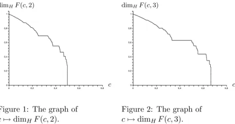
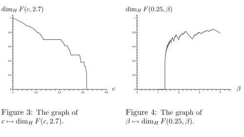
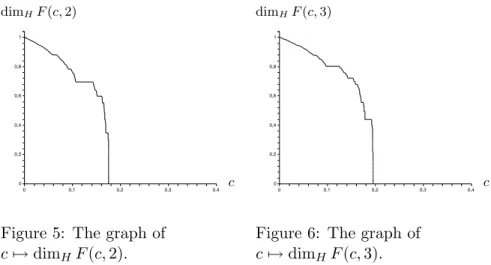
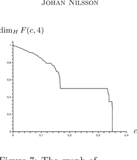
Figure
Documents relatifs